1. Introduction
The motion of large-scale flows in rotating planets is mostly confined in a two-dimensional (2-D) surface perpendicular to gravity. For instance, oceans are often modelled as a 2-D flow on a sufficiently large plane tangent to the Earth's surface, and planetary atmospheres are considered to flow over a spherical shell (see e.g. Vallis Reference Vallis2017, p. 66). Although many geophysical flows are highly turbulent and show complicated patterns, they often present coherent structures that can be represented with analytical solutions of 2-D vortex models. Classic examples are the nonlinear solutions of the 2-D Euler equations for monopolar (Rankine, Kirchoff), dipolar (Lamb, Chaplygin) and elliptical (Kida) vortices. A comprehensive account of some of these structures was given by Meleshko & van Heijst (Reference Meleshko and van Heijst1994). In the quasi-geostrophic (QG) context, Stern (Reference Stern1975) (see also Flierl, Stern & Whitehead Reference Flierl, Stern and Whitehead1983) derived the so-called ‘modons’, which turn out to be a particular class of the Chaplygin dipole (Meleshko & van Heijst Reference Meleshko and van Heijst1994). Recently, Viúdez (Reference Viúdez2019a,Reference Viúdezb) provided azimuthal-mode solutions of multipolar 2-D Euler and baroclinic QG vortices.
In this paper, we discuss analytical nonlinear solutions of vortices trapped over variable topography. In a rotating reference frame, inviscid topography effects promote the formation of vortices owing to the conservation of potential vorticity (Huppert & Bryan Reference Huppert and Bryan1976). Over a submarine mountain, for instance, anticyclonic vorticity is generated on the summit owing to squeezing effects, whereas fluid columns moving downward are stretched hence generating cyclonic vorticity (Verron & Le Provost Reference Verron and Le Provost1985). The flow dynamics are usually incorporated in shallow-water models (Grimshaw, He & Broutman Reference Grimshaw, He and Broutman1994). When the topographic variations are small with respect to the mean fluid depth, the model is reduced to the barotropic QG equations (Carnevale et al. Reference Carnevale, Purini, Orlandi and Cavazza1995). A review of the 2-D dynamics with topography and several experimental applications can be found in Zavala Sansón & van Heijst (Reference Zavala Sansón and van Heijst2014).
Organised motions over the topography may remain trapped during long periods while maintaining a well-defined structure. Such a striking phenomenon led Hide (Reference Hide1961) to suggest that Jupiter's Great Red Spot might be a manifestation of a columnar vortex over a ‘topographical feature’ of the surface underlying the atmosphere (a hypothesis that was soon discarded). More recently, Zavala Sansón, Aguilar & van Heijst (Reference Zavala Sansón, Aguilar and van Heijst2012) performed laboratory experiments in a large rotating tank, in which cyclonic vortices approached a submerged mountain. The most relevant result was the formation of an asymmetric cyclone–anticyclone pair rotating around the mountain. The authors noted that such a structure was similar to mode-1 topographic waves around an axisymmetric topography (Zavala Sansón Reference Zavala Sansón2010).
The most relevant solutions in this study are dipolar vortices over isolated topographies in a QG flow. The structures are similar to the Chaplygin vortex, which may be either symmetric and moving along a straight line, or asymmetric and drifting on a circular path (Meleshko & van Heijst Reference Meleshko and van Heijst1994). Dipoles may be asymmetric owing to bottom friction effects, as shown in more recent experimental, numerical and theoretical studies (Zavala Sansón, van Heijst & Backx Reference Zavala Sansón, van Heijst and Backx2001; Makarov Reference Makarov2012). In contrast, the asymmetry in our case is due to the shape of the variable bottom, and the dipoles remain attached to the topography while slowly rotating around it. To obtain the solutions, we follow a similar approach to that of Viúdez (Reference Viúdez2019a): using polar coordinates, the interior (over the topography) stream function is separable, where an infinite set of azimuthal modes comprises the azimuthal part. The crucial difference in our approach is the consideration of an additional term associated with the presence of an axisymmetric bump or depression. The dipoles are steady, nonlinear solutions of the QG dynamics in a reference frame that rotates with the vortex. The rotary motions of the dipole depend entirely on the characteristics of the topography.
The paper is organised as follows. In § 2, we present the interior solutions for multipolar vortices; then, we introduce the exterior flow for modes  $m=0$ and 1. Explicit formulae are derived for the angular speed of dipolar modes and the condition to remain trapped around the topography. Section 3 evaluates the structure of monopolar and dipolar solutions for a specific set of topographies. In addition, numerical solutions are performed to evaluate the analytical results. In § 4 the results are summarised and discussed.
2. QG solutions with axisymmetric topography
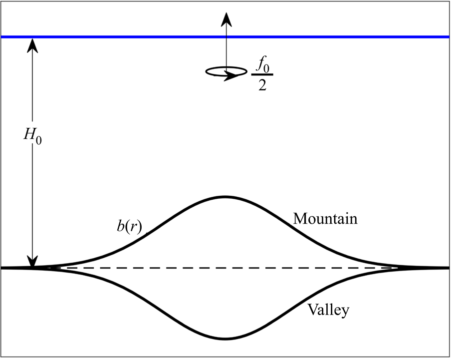
Consider a barotropic, incompressible and inviscid fluid in a QG regime on the  $f$-plane, above a localised axisymmetric submarine mountain or valley (see figure 1). Using a polar coordinate system
  $(r,\theta )$, the potential vorticity equation is (see e.g. Vallis Reference Vallis2017, pp. 207–211)
 \begin{equation} \frac{\partial}{\partial t}\nabla^2 \psi + \textrm{J}[\psi,\nabla^2 \psi + h(r)]=0, \end{equation}
where  $\omega = \nabla ^2 \psi$ is the relative vorticity with
  $\psi$ a stream function,
  $h(r)=f_0b(r)/H_0$ is the ambient vorticity with
  $b(r)$ the topography centred at
  $r=0$,
  $f_0$ the Coriolis parameter and
  $H_0$ the average depth of the fluid layer. The Jacobian operator is
  $\textrm {J}(a,b)\equiv (a_{r}b_{\theta } - a_{\theta }b_{r})/r$ and the Laplacian
  $\nabla ^2 a= a_{rr} +a_r/r + (1/r^2)a_{\theta \theta }$, where the
  $r,\theta$ subscripts indicate partial derivatives. The radial and azimuthal components of the velocity are defined as
  $u=-\psi _{\theta }/r$ and
  $v=\psi _{r}$, respectively. The potential vorticity is defined as
 \begin{equation} q=\nabla^2 \psi + h = \omega + h. \end{equation}
According to (2.1),  $q$ is materially conserved.

Figure 1. Side view of a homogeneous fluid layer over an axially symmetric submarine mountain or valley  $b(r)$, on an
  $f$-plane with mean depth
  $H_0$.
2.1. Azimuthal modes over topography
We seek solutions of the vorticity equation (2.1) based on the azimuthal-mode decomposition used by Viúdez (Reference Viúdez2019a) (hereafter referred to as V19), who studied the purely 2-D case, i.e. with  $h(r)=0$. In the presence of topography,
  $h(r)\neq 0$, we propose a stream function with two terms
 \begin{equation} \psi_{m} (r,\theta) =\psi_{Vm}(r,\theta)+\phi (r), \end{equation}
where
 \begin{equation} \psi_{Vm}(r,\theta) = Re\left[ \hat{\psi}_m\textrm{J}_{m}(c_0r)\textrm{e}^{\textrm{i}m \theta} \right] \end{equation}
are the V19 steady solutions for azimuthal modes  $m$ (
$m$ ( $=0,1,\ldots$) in the absence of topography,
  $\textrm {J}(\psi _{Vm},\nabla ^2\psi _{Vm})=0$. The complex amplitudes
  $\hat {\psi }_m$ define the vortex strength and orientation,
  $\textrm {J}_m$ is the Bessel function of the first kind of order
  $m$ and
  $c_0$ a scaling factor for the radial coordinate with units 1/length. The topography effects are included in
  $\phi (r)$, which is assumed purely radial owing to the symmetry of the submarine mountain or valley. To obtain an explicit expression for
  $\phi (r)$, we replace (2.3) in the vorticity equation (2.1), which yields
 \begin{equation} -\frac{\partial \psi_{Vm}}{\partial \theta} \frac{\textrm{d}}{\textrm{d}r}\left(\frac{\textrm{d}^2\phi}{\textrm{d}r^2} + \frac{1}{r} \frac{\textrm{d}\phi}{\textrm{d}r} + c_0^2 \phi + h \right) = 0, \end{equation}
where we have used that  $\nabla ^2\psi _{Vm}=-c_0^2\psi _{Vm}$. Hence, to satisfy this expression for any mode
  $m$ it is sufficient that function
  $\phi (r)$ obeys the second-order equation
 \begin{equation} \frac{\textrm{d}^2\phi}{\textrm{d}r^2} + \frac{1}{r} \frac{\textrm{d}\phi}{\textrm{d}r} + c_0^2 \phi + h = h_0, \end{equation}
where  $h_{0}$ is a constant. In terms of the dimensionless coordinate
  $s=c_0r$, equation (2.6) transforms into
 \begin{equation} \frac{\textrm{d}^2\phi}{\textrm{d}s^2} + \frac{1}{s} \frac{\textrm{d}\phi}{\textrm{d}s} + \phi = \frac{h_0-h(s)}{c_0^2} \equiv H(s). \end{equation}
The function  $H(s)$ contains the information about the topography, and its magnitude is of order
  $h_0/c_0^2$ (with the same units as the stream function). It is convenient to choose
  $h_0=h(0)$ so that
  $H$ is zero at the origin. In addition, note that
  $H=0$ in the absence of topography.
The general solution of (2.7) is the sum of the homogeneous and a particular solution. The homogeneous form of (2.7) is a Bessel equation, whose general solution is a linear combination of the zero-order Bessel functions of the first and second kind,  $\textrm {J}_{0}(s)$ and
  $\textrm {Y}_{0}(s)$, respectively. We require the solutions to be finite at
  $s = 0$, so the homogeneous solution only involves
  $\textrm {J}_{0}(s)$. In addition, a particular solution of (2.7) can be obtained via the standard method of variation of parameters. Thus, the general solution is
 \begin{align} \phi(s) = \frac{h_0}{c_0^2} C \textrm{J}_{0}(s)+ \textrm{Y}_{0}(s)\int_{0}^{s} \frac{H(s')\textrm{J}_{0}(s')}{W\left[\textrm{J}_{0}(s'),\textrm{Y}_{0}(s')\right]}\,\textrm{d}s' - \textrm{J}_{0}(s)\int_{0}^{s} \frac{H(s')\textrm{Y}_{0}(s')}{W\left[\textrm{J}_{0}(s'),\textrm{Y}_{0}(s')\right]}\,\textrm{d}s', \end{align}
where  $W=\textrm {J}_0\textrm {Y}'_0-\textrm {Y}_0\textrm {J}'_0$ is the Wronskian. The first term represents the homogeneous solution, which is an axisymmetric structure with amplitude
  $h_0/c_0^2$ modulated by the arbitrary, dimensionless constant
  $C$. For convenience, we assume that this constant is different for each mode
  $m$ and will be denoted as
  $C_{m}$.
The last two terms are a particular solution, which can be rewritten applying the Wronskian identity of the Bessel functions,  $W[\textrm {J}_{0}(s),\textrm {Y}_{0}(s)]=2/{\rm \pi} s$ (Watson Reference Watson1986, p. 76). Thus,
 \begin{equation} \phi(s) = \frac{h_0}{c_0^2} C_m \textrm{J}_{0}(s)+ \frac{\rm \pi}{2}\textrm{Y}_{0}(s)\int_{0}^{s} H(s')\textrm{J}_{0}(s')s'\,\textrm{d}s' - \frac{\rm \pi}{2}\textrm{J}_{0}(s)\int_{0}^{s} H(s')\textrm{Y}_{0}(s')s' \,\textrm{d}s'. \end{equation}
Using (2.9) in (2.3), we obtain steady solutions of the QG model with axisymmetric topography over the whole plane. However, to obtain a physically meaningful vortical structure with bounded vorticity, it is required to restrict the solutions within an interior region above the localised topography and to determine a suitable potential flow in the exterior domain.
2.2. Interior flow
The interior vortex solutions (denoted with subindex  $I$) within a circular region with radius
  $s_{l}$ (defined in the following) are
 \begin{align} \psi_{Im}(s,\theta) &= Re\left[\hat{\psi}_m\textrm{J}_{m}(s)\textrm{e}^{\textrm{i} m \theta}\right] + \frac{h_0}{c_0^2} C_m \textrm{J}_{0}(s) +\frac{\rm \pi}{2}\textrm{Y}_{0}(s)\int_{0}^{s} H(s')\textrm{J}_{0}(s')s'\,\textrm{d}s' \nonumber\\ &\quad - \frac{\rm \pi}{2}\textrm{J}_{0}(s)\int_{0}^{s} H(s')\textrm{Y}_{0}(s')s' \,\textrm{d}s', \quad s\leq s_l. \end{align}
The velocity field (expressed in terms of the unit vectors  $\widehat {\boldsymbol {e}_r}$ and
  $\widehat {\boldsymbol {e}_{\theta }}$) and the relative vorticity are calculated directly:
 \begin{align} \frac{\boldsymbol{u}_{Im}(s,\theta)}{c_0} &={-}\frac{m}{s}Re\left[ \textrm{i}\hat{\psi}_{m}\textrm{J}_{m}(s)\textrm{e}^{\textrm{i}m\theta}\right] \widehat{\boldsymbol{e}_r} + \left[ Re \left[\hat{\psi}_{m}\textrm{J}'_{m}(s)\textrm{e}^{\textrm{i}m\theta}\right] - \frac{h_0}{c_0^2} C_{m}\textrm{J}_{1}(s) \right.\nonumber\\ &\quad - \left.\frac{{\rm \pi} \textrm{Y}_{1}(s)}{2}\int_{0}^{s} H(s')\textrm{J}_{0}(s')s'\,\textrm{d}s'+\frac{{\rm \pi} \textrm{J}_{1}(s)}{2}\int_{0}^{s} H(s')\textrm{Y}_{0}(s')s'\,\textrm{d}s'\right]\widehat{\boldsymbol{e}_{\theta}},\quad s\leq s_l, \end{align}
 \begin{align}\frac{\omega_{Im}(s,\theta)}{c_0^2} &={-}Re\left[\hat{\psi}_m\textrm{J}_{m}(s)\textrm{e}^{\textrm{i}m \theta}\right] - \frac{h_0}{c_0^2} C_{m}\textrm{J}_{0}(s)- \frac{\rm \pi}{2}\textrm{Y}_{0}(s)\int_{0}^{s} H(s')\textrm{J}_{0}(s')s'\,\textrm{d}s'\notag\\ &\quad + \frac{\rm \pi}{2}\textrm{J}_{0}(s)\int_{0}^{s} H(s')\textrm{Y}_{0}(s')s' \,\textrm{d}s' + H(s), \quad s\leq s_l. \end{align}
Note from (2.10) and (2.12) that the vorticity is
 \begin{equation} \omega_{m}(s,\theta) = c_0^2 \left[ -\psi_m(s,\theta) + H(s)\right]. \end{equation}
Substituting  $H(s)$ from (2.7) it is also found that the potential vorticity is proportional to the stream function:
 \begin{equation} q(s,\theta) \equiv \omega_{m}(s,\theta) + h(s) ={-}c_0^2 \psi_m(s,\theta) + h_0. \end{equation}
Later we will examine scatter plots to verify that the analytical solutions indeed obey a linear  $q$ versus
  $\psi$ relationship.
Following V19, the radial distance  $s_l$ to confine the vortex can be chosen as one of the
  $n$ (
$n$ ( $\geq 1$) zeros of the
  $m$-Bessel function,
  $j_{m,n}$. A suitable choice is
  $s_l=j_{1,1}=3.8317$ (the first zero of
  $\textrm {J}_1$), because there the radial velocity component becomes zero (see (2.11)).
Modes  $m=0$ and
  $1$ represent monopolar and dipolar vortices modified by the topography, which are the relevant cases to study from now on. In the 2-D case, the monopoles may be cyclonic (
 $\hat {\psi }_0<0$) or anticyclonic (
 $\hat {\psi }_0>0$), with
  $\hat {\psi }_0$ real. For dipoles, the real and imaginary parts of
  $\hat {\psi }_1$ indicate the vortex amplitude and orientation.
2.3. Complete solutions for mode  $m=0$
$m=0$

To complete the solutions, one needs to add an exterior flow, so the interior vorticity distribution remains confined over the topography. For the monopolar mode  $m=0$, we set the exterior stream function as the sum of an irrotational (logarithmic) profile and a constant-vorticity, quadratic term (V19). The exterior axisymmetric solution (denoted with subindex
  $E$) is
 \begin{equation} \psi_{E0}(s)=a_{0}+a_{1}\ln s+a_{2}s^2, \quad s \ge s_{l}, \end{equation}
where the coefficients are chosen to satisfy the continuity of the stream function, the azimuthal velocity and the vorticity.
The matching conditions at the boundary  $s_l$ are
 \begin{equation} \left. \begin{gathered} \psi_{I0}|_{s_{l}} = \psi_{E0}|_{s_{l}},\\ \psi'_{I0}|_{s_{l}} = \psi'_{E0}|_{s_{l}},\\ \left[\psi''_{I0}+\frac{1}{s}\psi'_{I0}\right]_{s_{l}} = \left[\psi''_{E0}+\frac{1}{s}\psi'_{E0}\right]_{s_{l}}, \end{gathered} \right\} \end{equation}
(where primes indicate complete  $s$-derivatives). Using (2.10) and (2.15) in (2.16), we obtain the coefficients
  $a_{0}$,
  $a_{1}$ and
  $a_{2}$ in terms of the somewhat cumbersome constants
  $f_{00}$ and
  $f_{01}$ shown in Appendix A. Hence, the exterior fields for mode 0 are
 \begin{gather} \psi_{E0}(s) = f_{00}+\left[{-}f_{01}s_{l}+\frac{1}{2}(\,f_{00}-H(s_{l}))s_l^2 \right] \ln \left(\frac{s}{s_{l}}\right) \nonumber\\ -\frac{f_{00}-H(s_{l})}{4}\left(s^2-s_{l}^2 \right) \end{gather}
 \begin{gather}\frac{u_{E0}(s)}{c_0} = \left[{-}f_{01}\frac{s_{l}}{s} + \frac{1}{2}(\,f_{00}-H(s_{l}))\frac{s_{l}^2-s^2}{s}\right]\hat{\boldsymbol{e}}_{\theta} \end{gather}
 \begin{gather}\frac{\omega_{E0}}{c_{0}^{2}} ={-}[\,f_{00}-H(s_{l})] . \end{gather}
To check for dimensional consistency, note that the units of  $f_{00}$,
  $f_{01}$ and
  $H(s_l)$ are those of the stream function (length
 $^2$/time). The exterior vorticity
  $\omega _{E0}$ is constant, corresponding with the added rotation.
The complete solution for mode  $m=0$ is
 \begin{equation} \psi_0(s) = \begin{cases} \psi_{I0}(s), & s \le s_l, \\ \psi_{E0}(s), & s \ge s_l, \end{cases} \end{equation}
which is stationary in a coordinate system that rotates with angular speed  $2a_2$.
In fact, equation (2.20) is a family of circular vortices expressed in different coordinate systems rotating according to the value of  $a_2$ (which depends on constants
  $H(s_{l})$ and
  $f_{00}$, see (2.19)). In particular, the exact solution in the original
  $f$-plane is
 \begin{equation} \psi_0(s) = \begin{cases} \psi_{I0}(s) - a_0 - a_2 s^2, & s \le s_l, \\ a_{1}\ln s, & s \ge s_l, \end{cases} \end{equation}
in which the exterior vorticity is zero.
2.4. Complete solutions for mode $m=1$

For convenience, hereafter we use the dipole amplitude as  $\hat {\psi }_1=-|\hat {\psi }_1|i$, so the V19 mode is
  $|\hat {\psi }_1|\textrm {J}_{1}(s)\sin (\theta )$. This case corresponds with a dipole initially oriented in the horizontal direction and pointing to the left in a planar system.
Before discussing the exterior solution, we assume first that the whole dipolar mode rotates steadily around the topography. We therefore seek solutions at a rotating reference frame such that  $\psi =\psi (s,\theta +\varOmega t$), where the rotation is clockwise (anticlockwise) for
  $\varOmega >0$ (
 $\varOmega <0$). For the moment,
  $\varOmega$ remains unknown. The vorticity equation becomes (Flierl et al. Reference Flierl, Stern and Whitehead1983)
 \begin{equation} \textrm{J}\left[\psi(s,\theta)+ \frac{\varOmega}{2 c_0^2} s^2,\nabla^{2} \psi(s,\theta) + h(s)\right]=0, \end{equation}
keeping in mind that now  $\theta$ corresponds to the rotated azimuthal coordinate. Thus, the solutions for mode 1 are of the form
 \begin{equation} \psi_1(s,\theta) = \begin{cases} \psi_{I1}(s,\theta) - \dfrac{\varOmega}{2 c_0^2} s^2, & s \le s_l, \\ \psi_{E1}(s,\theta), & s \ge s_l, \end{cases} \end{equation}
where  $\psi _{E1}(s,\theta )$ is the exterior field. The vorticity is
 \begin{equation} \omega_1(s,\theta) = \begin{cases} \omega_{I1}(s,\theta) - 2\varOmega, & s \le s_l, \\ - 2\varOmega, & s \ge s_l. \end{cases} \end{equation}
Now we can construct the exterior solution with the desired properties. The exterior field is proposed as the sum of a non-axisymmetric potential component and a symmetric flow similar to (2.15):
 \begin{equation} \psi_{E1}(s,\theta)=\frac{U_0}{c_0}\left(s-\frac{s_{l}^2}{s}\right)\sin \theta +d_0 + d_1 \ln s + d_2s^2, \quad s \ge s_{l}, \end{equation}
where  $U_{0}$ is an additional constant to be determined, and coefficients
  $d_0$,
  $d_1$ and
  $d_2$ are chosen to ensure that the flow variables are continuous at
  $s_l$. An equivalent procedure was first proposed by Chaplygin (Reference Chaplygin1903) to derive steady solutions of 2-D asymmetric dipoles travelling along circular paths with speed
  $U_0$ (Meleshko & van Heijst Reference Meleshko and van Heijst1994). In the present case, the whole dipolar mode may rotate but cannot translate because it remains attached to the topography.
From (2.23), the matching conditions are
 \begin{equation} \left. \begin{gathered} \psi_{I1}|_{s_{l}} -\frac{\varOmega}{2 c_0^2}s_l^2 = \psi_{E1}|_{s_{l}},\\ \partial_s \psi_{I1}|_{s_{l}} - \frac{\varOmega}{c_0^2} s_l = \partial_s \psi_{E1}|_{s_{l}},\\ \left[\partial_{ss} \psi_{I1}+\frac{1}{s}\partial_s \psi_{I1}+\partial_{\theta\theta} \psi_{I1}\right]_{s_{l}} -\frac{2\varOmega}{c_0^2} = \left[ \partial_{ss} \psi_{E1}+\frac{1}{s}\partial_s \psi_{E1} +\frac{1}{s^2}\partial_{\theta \theta}\psi_{E1} \right]_{s_{l}}. \end{gathered} \right\} \end{equation}
The form of the exterior flow (2.25) ensures that the condition for the  $\theta$-derivative of the stream function is identically satisfied. System (2.26) is solved to obtain the coefficients of the exterior field, as shown in Appendix B. In particular, it is found that coefficient
  $d_2$ is predetermined by the rotation
  $\varOmega$, such that
  $d_2=-\varOmega /(2c_0^2)$, which can be proved immediately from (2.24) and (2.25). An additional consequence is that the constant
  $C_1$ found in the interior solution must have a specific value given by (B6) to satisfy continuity of the vorticity. The other coefficients,
  $d_0$ and
  $d_1$, depend on constants
  $f_{10}$ and
  $f_{11}$, which contain integrals of
  $H(s)$ and therefore they are of order
  $h_0/c_0^2$. In addition,
  $U_0$ is proportional to the amplitude
  $|\hat {\psi }_1|$, see (B4). The exterior fields are
 \begin{align} \psi_{E1}(s,\theta) &= \frac{1}{2}|\hat{\psi}_1|\textrm{J}'_1(s_l)\left(s-\frac{s_{l}^2}{s}\right) \sin \theta + \,f_{10} -\,f_{11}s_{l} \ln \left(\frac{s}{s_{l}}\right) -\frac{\varOmega}{2c_0^2}s^2, \end{align}
 \begin{align} \frac{u_{E1}(s,\theta)}{c_0} &= \left[-\frac{1}{2}|\hat{\psi}_1|\textrm{J}'_{1}(s_l)\left(1-\frac{s^2_{l}}{s^2}\right) \cos \theta\right]\hat{\boldsymbol{e}}_{r} \nonumber\\ &\quad + \left[\frac{1}{2}|\hat{\psi}_1|\textrm{J}'_{1}(s_l)\left(1+\frac{s^2_{l}}{s^2}\right) \sin \theta -\,f_{11}\frac{s_{l}}{s} -\frac{\varOmega}{c_0^2}s \right]\hat{\boldsymbol{e}}_{\theta}, \end{align}
 \begin{align}&\hspace{8pc}\frac{\omega_{E1}}{c_{0}^{2}} ={-}2\varOmega . \end{align}
Dipolar solutions imply a special restriction for the topography because the exterior field evaluated in the vorticity equation (2.22) yields
 \begin{equation} \textrm{J}\left[\frac{U_0}{c_0}\left(s-\frac{s_{l}^2}{s}\right)\sin \theta,h(s)\right] = 0, \quad s > s_{l}. \end{equation}
Therefore, the exterior dipolar solutions are valid for isolated topographic features vanishing outwards:
 \begin{equation} \frac{\textrm{d}h(s)}{\textrm{d}s} = 0, \quad s > s_{l}. \end{equation}
In other words, the topography must decay rapidly within the vortex interior. Note that this restriction does not apply for the axisymmetric mode  $0$.
$0$.
2.5. Angular speed of dipolar modes
The angular speed of the dipole on the  $f$-plane is
  $-\varOmega$. To obtain
  $\varOmega$, it is noted that the total circulation of the interior region (2.24) must be zero. The circulation is calculated as the area integral of the interior potential vorticity:
 \begin{equation} \varGamma_I=\int_0^{2{\rm \pi}} \int_0^{s_l} \left[\omega_{I1}(s,\theta) - 2\varOmega + h(s) \right] c_0^{{-}2} s\,\textrm{d}s \,\textrm{d}\theta. \end{equation}
The first integral is calculated as the line integral of the tangential velocity:
 \begin{equation} \int_0^{2{\rm \pi}} \int_0^{s_l} \omega_{I1}(s,\theta) c_0^{{-}2} s\,\textrm{d}s\,\textrm{d}\theta = \oint \partial_s \psi_{I1}(s_l,\theta) s_l \,\textrm{d}\theta ={-}2{\rm \pi} s_l f_{11}, \end{equation}
where constant  $f_{11}$ is defined by (B3). Solving the other integrals, the circulation is
 \begin{equation} \varGamma_I={-}2{\rm \pi} s_l f_{11} - {\rm \pi}s_l^2 c_0^{{-}2} 2 \varOmega + 2{\rm \pi} c_0^{{-}2} \int_0^{s_l} h(s)s\,\textrm{d}s. \end{equation}
Setting  $\varGamma _I=0$ and after straightforward calculations, it is found that
 \begin{equation} \varOmega = \left[-\frac{f_{11} c_0^2}{s_l} + \frac{1}{s_l^2} \int_0^{s_l} h(s)s\,\textrm{d}s \right]. \end{equation}
It must be remarked that  $\varOmega$ depends on the shape and properties of the topography.
2.6. Dipole entrapment
Now we examine the conditions that determine the attachment of the dipolar mode to the topography. This entrapment is equivalent to the problem of a rotating cylinder of radius  $r_l$ with circulation
  $\varGamma$ in a potential exterior flow with far-field velocity
  $U_0$ (Batchelor Reference Batchelor1967, pp. 539–540). The azimuthal velocity at the cylinder is
  $v(r_l,\theta )=2U_0 \sin \theta - \varGamma /(2{\rm \pi} r_l)$, so there may be stagnation points over the cylinder when
  $\sin \theta =\varGamma /(4{\rm \pi} U_0r_l)$. The absence of stagnation points requires
  $|\varGamma /(4{\rm \pi} U_0r_l)|>1$ for any
  $\theta$, that is, the circumferential velocity of the cylinder is always greater than
  $2 U_0$ (Spurk & Aksel Reference Spurk and Aksel2008, p. 367).
In the present case, in which we have introduced an additional rotation to the reference system, the tangential velocity at the boundary given by the exterior field is
 \begin{equation} v(s_l,\theta)= c_0 \frac{\partial}{\partial s} \psi_{E1}(s_l,\theta) = 2U_0\sin \theta + \frac{d_1 c_0}{s_l} - \frac{\varOmega s_l}{c_0}. \end{equation}
The absence of stagnation points implies that
 \begin{equation} \left|\frac{-d_1 c_0/s_l + \varOmega s_l/c_0}{2U_0} \right| > 1. \end{equation}
Substituting  $d_1=-\,f_{11}s_l$ (see (B5)) and using (2.35), this condition may be rewritten as
 \begin{equation} \gamma \equiv \left|\frac{1}{2U_0s_l} \int_0^{s_l} h(s)s\,\textrm{d}s \right| > 1. \end{equation}
 The physical parameters of the dipolar mode are restricted to satisfy (2.38) to guarantee the capture of the vortex over the topography. The restriction depends on the ratio between the integral of the topographic term and the vortex strength (proportional to  $U_0$). Thus, the dipole remains trapped as long as the topographic effect is sufficiently strong to prevent its propagation.
3. Trapped vortices over mountains and valleys
To examine the structure of the mode solutions we choose the mean depth  $H_0=1$ and the Coriolis parameter
  $f_0=1$ with arbitrary units. The radial length scale is set to
  $c_{0}=1$. The solutions are valid for any arbitrary bottom topography
  $b(r)$ as long as it is axisymmetric and isolated (i.e. it tends to zero at large
  $r$, as in figure 1). Hereafter, we consider topographies of the form
 \begin{equation} b(s)={\pm} b_{0}\textrm{e}^{-(s/s_t)^{\alpha}}, \end{equation}
where  $+b_{0}$ (-
 $b_0$) is the height (depth) of the submarine mountain (valley),
  $s_{t}$ is the dimensionless width and
  $\alpha$ is a real number that measures the shape of the topography. For
  $\alpha =2$ the topography is Gaussian; for
  $\alpha \gg 2$ the topography is almost flat near the origin and changes abruptly to zero for
  $s>s_t$. The relative topographic amplitudes
  $b_0/H_0$ are varied between
  ${\pm }0.3$ (therefore the same for
  $h_0=f_0b_0/H_0$).
3.1. Monopolar modes $m=0$

The solutions for  $m=0$ are monopolar circular structures centred above a submarine mountain or valley. The sense of rotation depends on the sign of the real amplitude
  $\widehat {\psi _0}$ of the V19 mode and the topographic terms proportional to
  $h_0/c_0^2$, including the arbitrary, dimensionless constant
  $C_0$. To facilitate the analysis, the solutions are evaluated for Gaussian topographies (
 $\alpha =2$) with the same horizontal size as the vortices,
  $s_{t} = s_{l}\equiv 3.8317$.
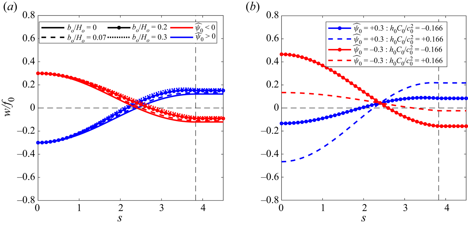
Figure 2 presents the radial vorticity profiles of vortices with  ${\pm }\hat {\psi }_0$ over mountains with (
 $a$) different amplitude
  ${\pm }b_0$ and fixed
  $C_0 = 0$, and (
 $b$) different constant
  ${\pm }C_0$ and fixed
  $b_0 = 0.2$. The profiles of cyclones and anticyclones for a given
  $b_0$ intersect at the first zero of
  $\textrm {J}_0$,
  $s=2.4048$, located in the interior region. Figure 2
 $(a)$ shows that the profiles have the same value at
  $s=0$, but are shifted upward for
  $s>0$. Thus, the vorticity is not symmetric with respect to the sign of
  $\hat {\psi }_0$ (compare the blue and red curves), except for the flat bottom case
  $b_0=0$. The radius of the zero crossing is smaller for anticyclones than for cyclones. Beyond that distance, the vorticity values are higher when
  $\hat {\psi }_0 > 0$ in comparison with the corresponding case with
  $\hat {\psi }_0 < 0$. At the exterior region,
  $s>s_l$, the vorticity reaches a constant value that corresponds with the negative of twice the rotation speed of the reference system in which all vortex modes are stationary.

Figure 2. Vorticity profiles for mode  $m=0$ over Gaussian mountains (
 $b_0>0$) using positive (blue) and negative (red) amplitude
  $\hat {\psi }_0={\pm }0.3$. The case of a flat bottom
  $b_0=0$ is also shown: (
 $a$)
$a$)  $C_0 = 0$ and
  $b_0/H_0= 0,0.07,0.2$ and
  $0.3$; (
 $b$)
$b$)  $C_0\pm 2$ and fixed
  $b_0/H_0=0.2$. The vertical dashed line indicates the radius of the interior–exterior boundary
  $s_l$.
Figure 2 $(b)$ presents the effect of
  $C_0\neq 0$ for
  $\pm \hat {\psi }_0$. For
  $C_0 > 0$, the vorticity profile of the anticyclone is amplified at both the core and the exterior (relative to the case
  $C_0 = 0$ in panel
  $a$), whereas the cyclone is weakened (dashed lines). The opposite occurs for
  $C_0 < 0$ (continuous curves): the anticyclone (cyclone) is weakened (amplified). On a valley (
 $b_0<0$), the vorticity profiles are equivalent to those in figure 2 when using
  $-\hat {\psi }_0$ and the same
  $C_0$. Thus, cyclones are intensified over valleys.
To reinforce the soundness of the proposed solutions, we examine scatter plots ( $q$ versus
  $\psi$) to verify the functional relationship between the potential vorticity and the stream function. Figure 3 shows well-defined
  $q$–
$q$– $\psi$ curves for all the solutions presented in figure 2: in each case, the linear relation corresponds to the interior region (
 $s < s_l$) predicted by (2.14), whereas the horizontal section is given by the exterior region (
 $s > s_l$).
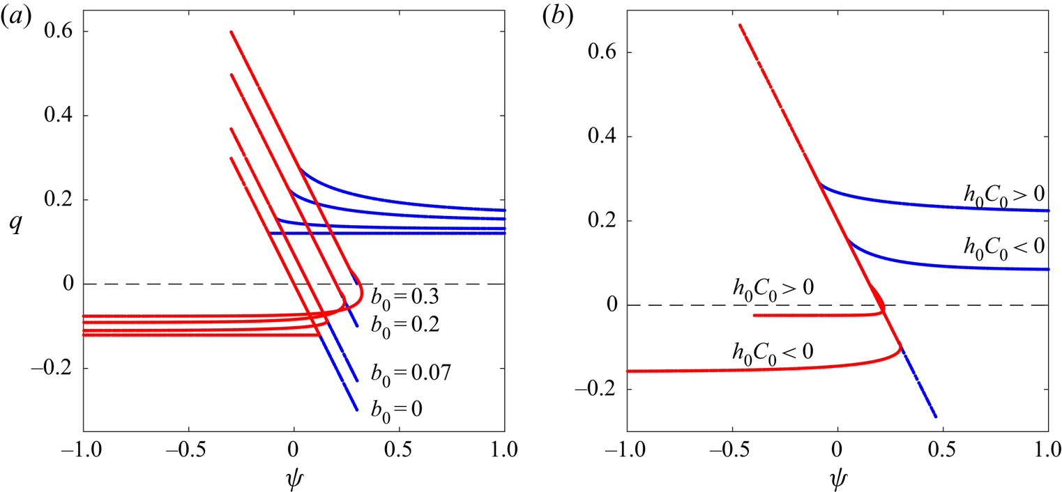
Figure 3. Scatter plots  $q$–
$q$– $\psi$ for modes
  $m=0$ shown in figure 2. In (
 $a$), values in the interior region are indistinguishable for a given
  $b_0$ (mountain,
  $h_0C_0/c_0^2 = 0$). In (
 $b$), all the interior regions are superposed (mountain,
  $b_0/H_0 = 0.2$).
3.2. Dipolar modes $m=1$

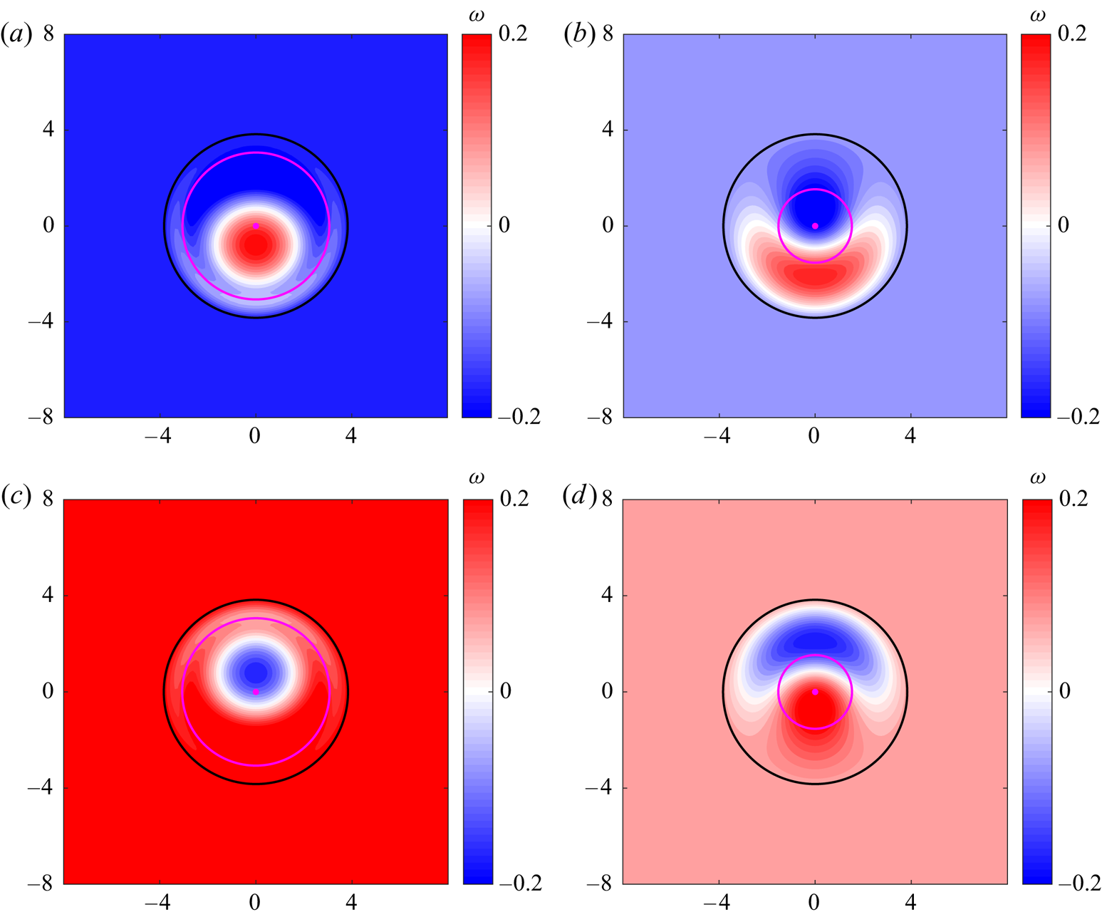
Now we examine the structure of steady dipolar vortices over the topography. Figure 4 shows representative vorticity distributions on a mountain ( $a{,}b$) and a valley (
 $c{,}d$), using the same vortex strength and topographic amplitude. The solutions differ on the shape and width of the topography: in (
 $a{,}c$) the topography decays abruptly before
  $s_l$, whereas in (
 $b,d$) the topography is Gaussian and narrow. In all cases, the vortices are asymmetric dipoles with different characteristics. Over the mountain, the dominant part of the dipole at the origin may be cyclonic when the topography is abrupt (
 $a$) or anticyclonic for the narrow mountain (
 $b$). In both cases, the exterior vorticity
  $-2\varOmega$ is negative, which indicates that the system has been rotated clockwise (
 $\varOmega >0$) to obtain steady solutions. Over the valley, dipoles have opposite attributes (panels
  $c{,}d$) so the structures rotate anticlockwise. Figure 5 presents the scatter plots of previous examples, in which it is verified the linear
  $q$–
$q$– $\psi$ relationship in the interior region.

Figure 4. Relative vorticity distributions of dipolar modes over different topographies.  $(a{,}b)$ Mountains with height
  $b_0 =0.2$:
  $(a)$ abrupt mountain;
  $(b)$ narrow mountain.
  $(c{,}d)$ Valleys with depth
  $b_0 = -0.2$:
  $(c)$ abrupt valley;
  $(d)$ narrow valley. For abrupt (narrow) topographies:
  $s_t=0.8s_l$,
  $\alpha =12$,
  $C_1=-1.59$ (
 $s_t=0.4s_l$,
  $\alpha =2$,
  $C_1=0.63$). In all cases the vortex strength is
  $|\hat {\psi }_1| = 0.3$. The black circumference corresponds to the interior–exterior vortex boundary at
  $s_l$. The radius of the magenta circle is the length scale of the topography
  $s_t$.
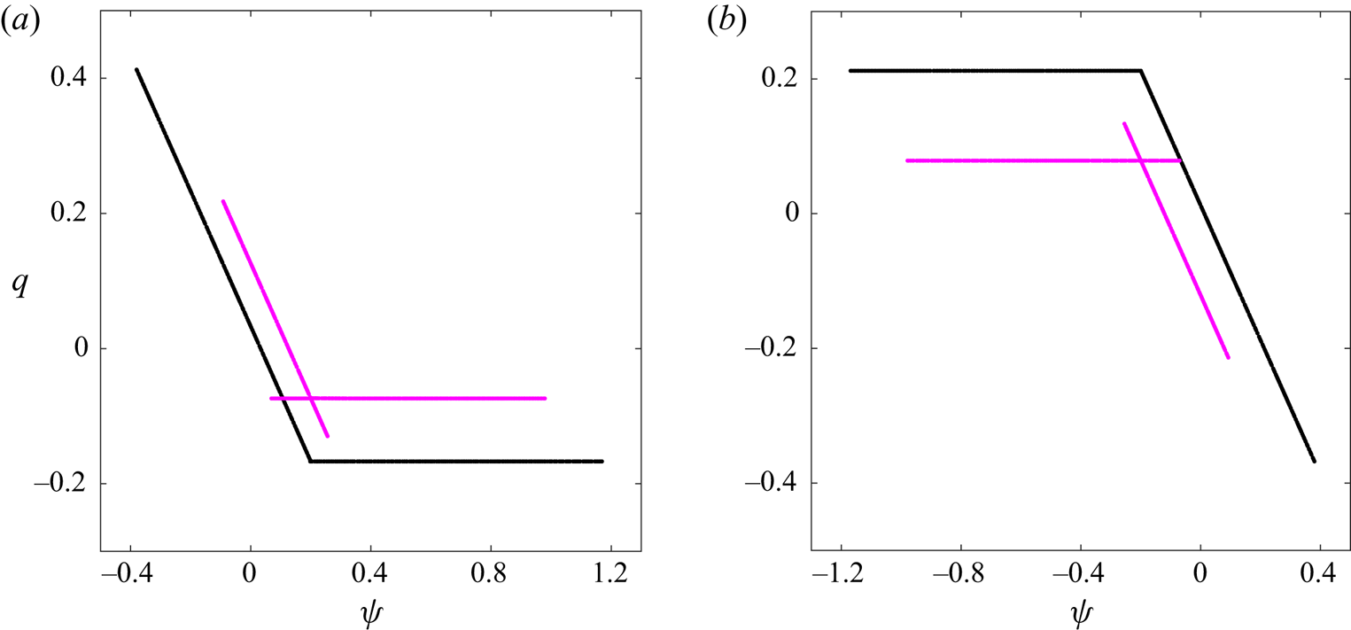
Figure 5. Scatter plots  $q$–
$q$– $\psi$ for modes
  $m=1$ corresponding to the examples shown in figure 4:
  $(a)$ mountains;
  $(b)$ valleys. Black (magenta) dots correspond to abrupt (narrow) topographies.
To better appreciate the structure of the solutions, figure 6 presents the stream function and the velocity fields corresponding to the dipoles shown in figure 4. The exterior vectors indicate the rotation seen from the reference frame fixed with the dipole. We added three  $\psi$ contours with values
  $[0.9,1,1.1]\psi _{E1}(s_l)$, which are useful to verify whether the streamlines enclose the vortex interior or they intersect the circular boundary at
  $s_l$ (magenta circle). In the former case, the vortices satisfy condition (2.38), so they are expected to remain attached to the topography. In contrast, when the flow parameters do not meet condition (2.38), then the vortices may escape and the solutions may not hold. In the examples with abrupt topographies (
 $a{,}c$), the streamlines enclosing the vortex are semi-circular, being slightly elongated in the vertical direction. In contrast, the streamlines in the examples over narrow topographies in (
 $b{,}d$) intersect the vortex boundary so that they may escape. The trapping condition is further explored with numerical simulations.
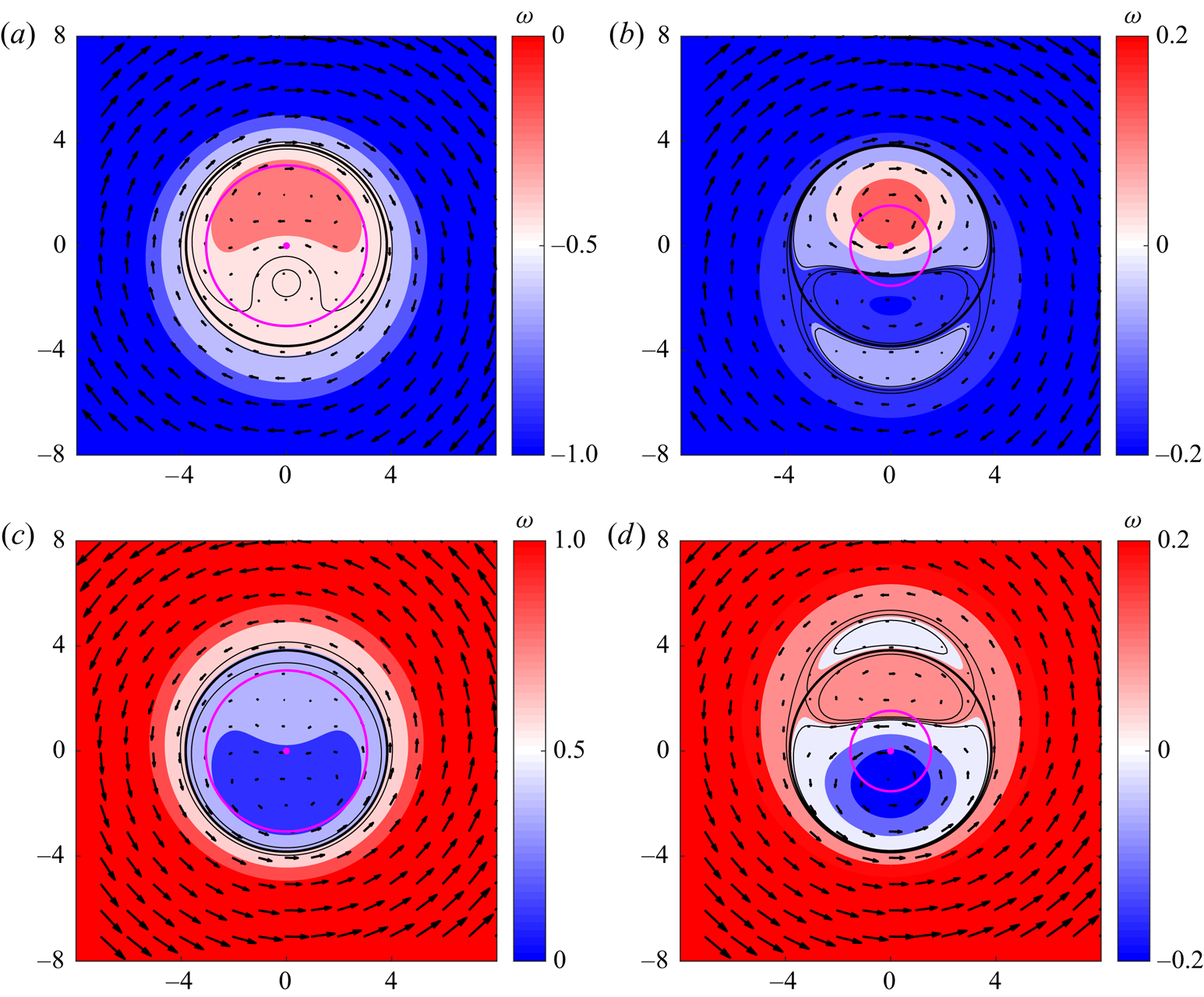
Figure 6. Stream function distributions and velocity fields of the dipolar modes shown in figure 4:  $(a)$ abrupt mountain;
  $(b)$ narrow mountain;
  $(c)$ abrupt valley;
  $(d)$ narrow valley. Black and magenta circles as in figure 4. Thin black lines indicate
  $\psi$-contours near the boundary with values
 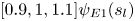 $[0.9,1,1.1]\psi _{E1}(s_l)$.
3.3. Numerical simulations
In this subsection, we present numerical experiments initialised with analytical vorticity fields. The analyses are mainly devoted to the dipolar mode  $m=1$ on the
  $f$-plane. The goal is to demonstrate that the analytical dipoles indeed rotate around the topography, clockwise over mountains and anticlockwise over valleys. We evaluate the theoretical angular speed and explore the behaviour of the solutions for different vortex and topography parameters.
3.3.1. Numerical code and flow parameters
The QG vorticity equation (2.1) is solved with a finite differences code analogous to those used in several previous studies on flows over variable bottom topography (Zavala Sansón & van Heijst Reference Zavala Sansón and van Heijst2014). A brief account is given here.
Initially, the vorticity distribution of a theoretical solution is prescribed on a square grid of length  $L$, with Cartesian coordinates
  $\{x,y|-L\leq x \leq L, -L\leq y \leq L\}$ and spatial resolution of
  $257 \times 257$ points. The initial stream function is obtained by inverting the Laplacian operator. Then, the time evolution of the vorticity is solved through a third-order Runge–Kutta scheme. Given the
  $f$-plane rotation period
  $T=4{\rm \pi} /f_0$, the time step is chosen as
  $dt=T/100$ to get sufficient temporal resolution for fluid motions within a ‘day’
  $T$. The typical duration of the simulations is
  $20T$. Once the new relative vorticity has been obtained, the process is repeated for subsequent times.
In all examples shown in the following, we set the basic parameters as in previous section:  $f_0=1$,
  $H_0=1$ and the dimensionless vortex radius
  $s_l=3.8317$. The scaled length is
  $L=16$, so the walls are sufficiently far away (about
  $4.2s_l$ from the origin) to minimise the image effect due to the free-slip boundaries. The initial condition is the vorticity field on the
  $f$-plane, which is obtained by subtracting the exterior vorticity
  $-2\varOmega$ to the steady solutions (2.24). Thus,
 \begin{equation} \omega_1(s,\theta,t=0) = \begin{cases} \omega_{I1}(s,\theta), & s \le s_l, \\ 0, & s \ge s_l. \end{cases} \end{equation}
3.3.2. Trapped vortices
The cases shown in this subsection satisfy condition (2.38), so the vortices remain trapped over the topography. The vortex solution for a steep mountain shown in figure 4 $(a)$ (also presented in figures 5
 $a$ and 6
 $a$) is a representative example of a steady dipole rotating around the topography on the
  $f$-plane. The trapping condition is
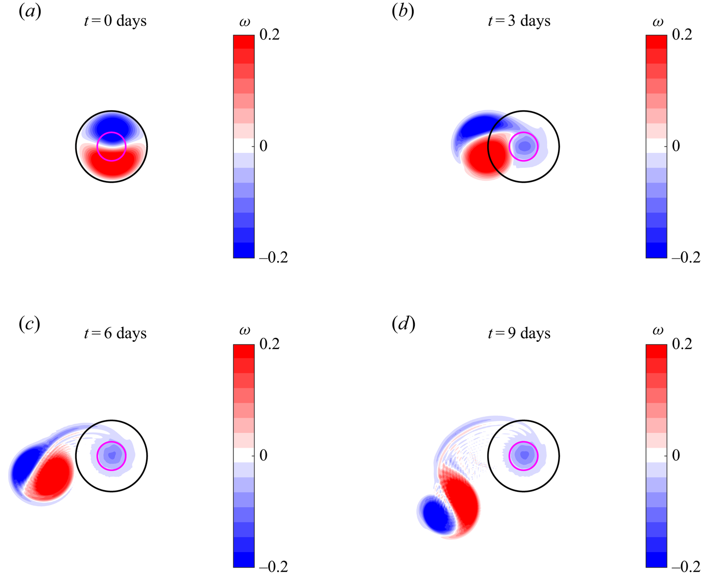
  $\gamma =1.88>1$. Figure 7 presents snapshots of the calculated vorticity distribution every two days, which illustrate the clockwise rotation of the whole structure. The expected rotation period is
  $5.4T$. As the initial configuration is almost recovered at day 6, this sequence shows that the numerical dipole rotates at a slightly lower speed. The steady vortex rotation during an extended period (20 days) is shown in Supplementary Movie 1 available at https://doi.org/10.1017/jfm.2021.85.
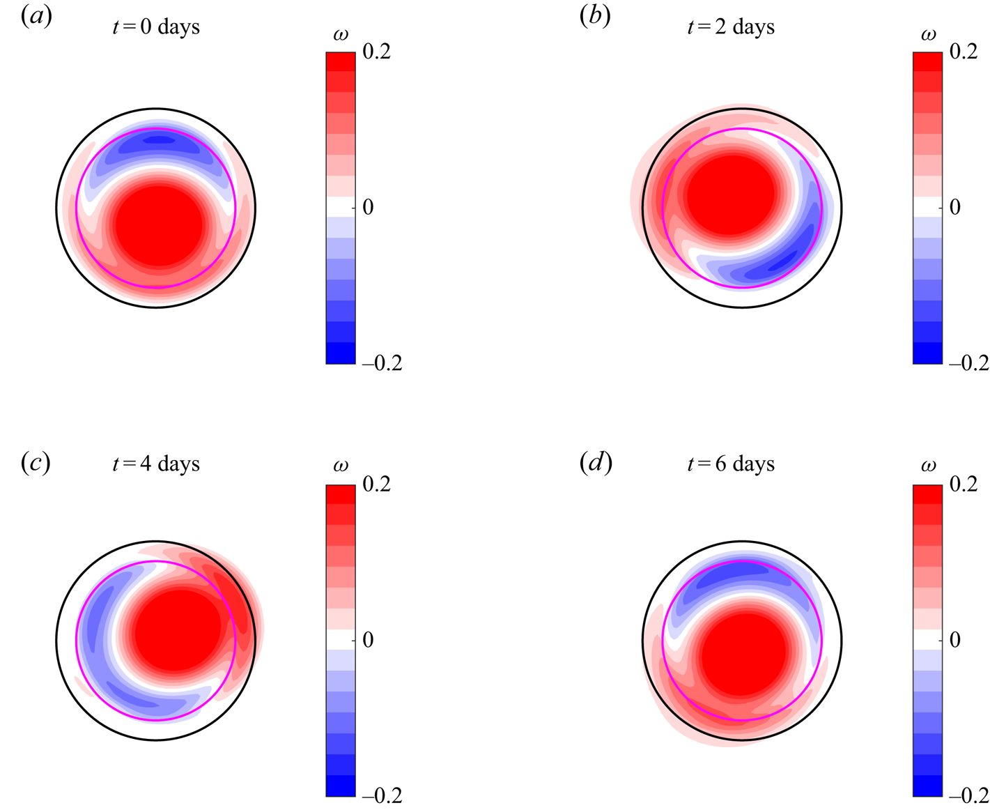
Figure 7. Sequence of numerically calculated vorticity distributions on the  $f$-plane of the asymmetric dipolar vortex shown in figure 4
 $(a)$. The topography is an abrupt mountain (
 $b_0=0.2$,
  $s_t=0.8 s_l$,
  $\alpha =12$). The dipole rotation is clockwise. The predicted angular speed is
 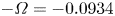 $-\varOmega =-0.0934$ with a period of 5.4 days.
We repeated the experiment for the same dipole but now over an equivalent valley (i.e. by setting  $b_0=-0.2$, as shown in figure 4
 $c$). The evolution of the vorticity distributions on the
  $f$-plane is shown in figure 8. As the remaining parameters are the same (including the trapping condition
  $\gamma =1.88$), the vortex angular speed is also the same, but now the rotation around the topography is anticlockwise. The
  $20$ days simulation is presented in Supplementary Movie 2.
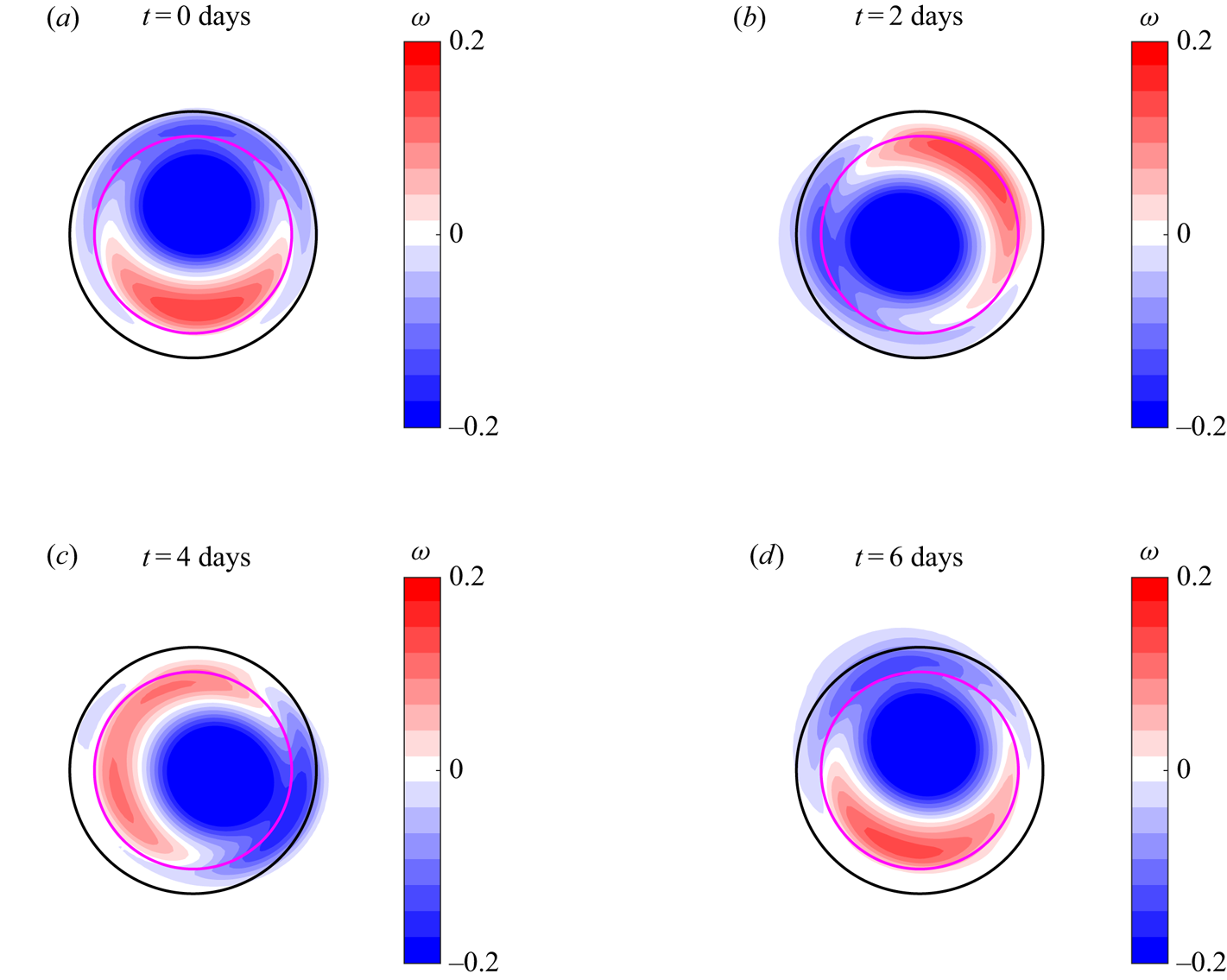


A third example is presented in figure 9, which shows a similar sequence of vorticity fields but now for a weaker dipole over a narrow, Gaussian mountain (inner circle). The trapping is condition  $\gamma =1.52$. The vortex steadily rotates clockwise and, as expected, the angular speed is slower than in previous case. Although the vortex remains trapped, it becomes clear that the structure is slightly distorted as time progresses. After several days, the main configuration remains though the structure continues eroding. Apparently, the mountain slope affects the structure of the analytical solution, probably due to the generation of topographic waves (in contrast with the nearly flat-topped mountain in figure 7). This point is discussed further in § 4.
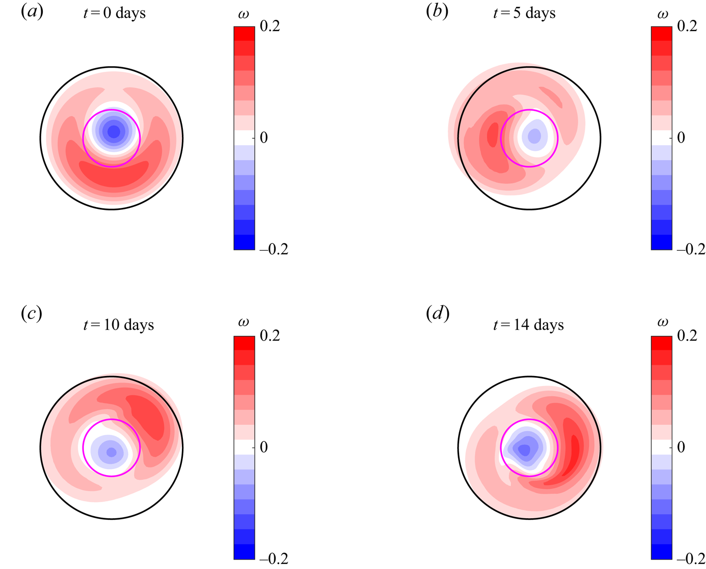
Figure 9. Sequence of vorticity distributions for a dipolar mode with  $|\hat {\psi }_1| = 0.1$. The topography is a narrow Gaussian mountain (
 $b_0=0.2$,
  $s_t=0.4 s_l$,
  $\alpha =2$,
  $C_1=0.63$). The dipole rotation is clockwise. The predicted angular speed is
  $-\varOmega =-0.0381$ with a period of 13.1 days.
3.3.3. Escaping vortex
When the analytical solutions do not satisfy the trapping condition (2.38), the vortices may escape away from the topography. This behaviour is shown in the sequence presented in figure 10 for a strong vortex over a mountain with a short height ( $b_0=0.1$). The vortex is sufficiently strong to overcome the topography effects, so the dipole drifts outside the interior region at early times. The emerging dipole is asymmetric, and its trajectory is bent towards the cyclonic side. Regardless of the fate of the dipole, it is evident that the analytical solution does not hold.

Figure 10. Sequence of numerically calculated vorticity distributions of an asymmetric dipolar vortex ( $|\hat {\psi }_1| = 0.6$) over a short mountain (
 $b_0=0.1$,
  $s_t=0.4 s_l$,
  $\alpha =2$). The trapping condition (2.38) is not satisfied:
  $\gamma =0.127$.
4. Discussion and conclusions
We have derived new analytical solutions for the nonlinear problem of an inviscid,  $f$-plane QG flow over isolated topography with axial symmetry. The solutions consist of an interior part over the topography, matched with an appropriate solution in the exterior region, where the topography becomes flat. The interior stream function is the sum of the azimuthal modes recently derived by Viúdez (Reference Viúdez2019a) for a 2-D flow and an axisymmetric function
  $\phi (s)$ representing the effects of the topography. The vortical structures are circular monopolar (
 $m=0$) and dipolar (
 $m=1$) modes. The corresponding V19 solutions are recovered when the bottom is flat, i.e.
  $\phi (s)\rightarrow 0$. A family of solutions is obtained from the competition between the vortex strength and the influence of the topographic parameters contained in
  $\phi (s)$. The number of possible solutions for
  $m=0$ is sensibly enhanced because
  $\phi (s)$ is composed by a circular structure with arbitrary amplitude
  $(h_0/c_0^2)C_0$, and additional terms involving the shape of the topography.
To illustrate the solutions, we used an exponential submarine mountain or valley with radial profile proportional to  $\exp (-s^{\alpha })$, where
  $\alpha$ is an arbitrary real number larger than one. These topographic features may be Gaussian (
 $\alpha =2$) or decay abruptly (
 $\alpha \gg 2$). The solutions also depend on both the height
  $b_0$ and width
  $s_t$ of the mountain or valley. For dipolar solutions, the topography must decay rapidly within the vortex interior.
The solutions are stationary in a reference frame that rotates with a constant angular speed depending on the topography. Monopolar modes are a special case because the sum of their circular flow and any other axisymmetric function is also a solution. As a consequence, the stream function may be expressed in any rotating system determined by a quadratic term imposed in the exterior field ( $a_2s^2$, see (2.15)).
Mode 1 solutions, on the other hand, consist of asymmetric dipolar vortices whose structure may be tuned by varying the flow parameters. The method to find the exterior field (far from the topography) is based on the procedure used originally by Chaplygin (Reference Chaplygin1903), who derived steady solutions of asymmetric dipoles travelling along circular paths. Meleshko & van Heijst (Reference Meleshko and van Heijst1994) showed the equivalence of this problem with that of a rotating cylinder immersed in a potential flow. An essential difference of the present results is that the dipoles remain trapped over the topography while rotating as a whole around the origin. An appropriate condition for having closed streamlines trapping the vortex (i.e. without stagnation points) was obtained in (2.38). The topography predetermines the rotation of the vortices. In general, dipoles rotate clockwise over mountains and anticlockwise over valleys. The sense of rotation is related with the local ‘westward’ direction imposed by the topography: along depth contours with shallow water to the right (for a Coriolis parameter  $f_0>0$). The angular speed
  $-\varOmega$ depends on the topographic parameters, as shown by (2.35).
The analytical solutions have been tested in two ways. First, by showing scatter plots that illustrate the linear dependence between the potential vorticity and the stream function predicted by (2.14). Second, through numerical simulations that solve the  $f$-plane, QG model initialised with analytical vorticity fields. We have presented examples of dipoles that remain trapped as predicted while rotating steadily around a mountain or valley (figures 7 and 8, and the supplementary movies), and also one case in which a dipole escapes from the influence of the topography (figure 10). In the latter example, the flow parameters did not satisfy criterion (2.38), so the self-propagating mechanism of the dipole was strong enough to overcome the topography effects.
A close inspection of the numerically calculated vorticity fields reveals that the shape of trapped vortices is slightly deformed. As a consequence, there was a short delay in the expected dipole rotation. Such effects were almost negligible over abrupt topographies and more evident over less steep slopes (as in figure 9). The simulations indicate that flow motions in the latter case are susceptible to perturbations that may trigger topographic Rossby waves, which are the natural oscillations in the QG dynamics with topography (Rhines Reference Rhines1969; Zavala Sansón, González-Villanueva & Flores Reference Zavala Sansón, González-Villanueva and Flores2010). Topographic waves are highly dispersive and, as a result, the erosion of dipoles over gentle slopes may be produced as the vortices radiate this type of oscillations. An equivalent process is well-known regarding the disintegration of translating monopolar vortices on the  $\beta$-plane owing to the radiation of planetary Rossby waves (see e.g. Carnevale, Kloosterziel & van Heijst Reference Carnevale, Kloosterziel and van Heijst1991). The origin of weak perturbations in our simulations may be associated with unavoidable numerical errors or to the resulting exterior far-field, which is slightly modified due to the straight boundaries of the square domain. Further analytical and numerical investigations are required to elucidate the conditions that lead to the vortex erosion, either due to wave radiation or to inherent instabilities of the analytical solutions.
Finally, we would like to point out that the generation of trapped vortices over isolated topography is a robust phenomenon observed in laboratory experiments. The formation of asymmetric dipole-like vortices over a submarine obstacle was qualitatively described in the rotating tank experiments of Carnevale et al. (Reference Carnevale, Kloosterziel and van Heijst1991). The structure was formed by a cyclonic vortex drifting over a conical hill along a nearly circular trajectory and a topographically generated anticyclonic patch over the summit. Similar experiments using a much larger tank and velocimetry measurements, Zavala Sansón et al. (Reference Zavala Sansón, Aguilar and van Heijst2012) reported the formation of nonlinear, asymmetric dipoles trapped over a submerged Gaussian mountain while rotating clockwise as a whole. The dipole asymmetry and the subinertial angular speed found in the present solutions closely resemble the experimental cases. For instance, the rotation periods of dipolar structures around the mountain in two different experiments of Zavala Sansón et al. (Reference Zavala Sansón, Aguilar and van Heijst2012) were approximately  $10.6$ and 4 ‘days’, where one day in the rotating platform was 30 s. The angular speeds were approximately
  $-0.05f_0$ and
  $-0.125f_0$, respectively (with
 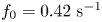 $f_0=0.42\ \textrm {s}^{-1}$; see their figures 6
 $b$ and 8). The angular speed of our analytical solutions is of the same order: in absolute value, we obtain
  $\varOmega$ between about
  $10^{-2}f_0$ and
  $10^{-1} f_0$. Some discrepancies are expected because the experimental dipoles have a more irregular shape as they arise from a very complex vortex–topography interaction. Thus, the observed vortices may not meet some characteristics of the theoretical solutions, such as the perfectly circular shape of the dipole atmosphere or the net-zero circulation over the mountain.
Considering the nonlinear nature of the experimental flows and the theoretical solutions, a plausible hypothesis is that strong perturbations over mountains may generate dipolar structures rotating clockwise. Consequently, the rotation of dipoles generated over valleys would be anticlockwise. We hypothesise that the newly formed vortices over isolated topography have a structure that is captured by the present solutions. This line of research is currently under investigation (Zavala Sansón & Gonzalez Reference Zavala Sansón and Gonzalez2021).
Supplementary movies
Supplementary movies are available at https://doi.org/10.1017/jfm.2021.85.
Acknowledgements
Comments and helpful suggestions from A. Viúdez and G. van Heijst are gratefully acknowledged.
Funding
J.F.G. thanks the support from the Consejo Nacional de Ciencia y Tecnología (CONACYT, México) and from the Secretaría de Educación de Bogotá (Colombia).
Declaration of interests
The authors report no conflict of interest.
Appendix A. Monopolar mode coefficients
The matching conditions (2.16) are written as
 \begin{equation} \left. \begin{gathered} f_{00} = a_{0}+a_{1} \ln s_{l}+a_2s_{l}^2,\\ -\,f_{01} = \frac{a_{1}}{s_{l}}+2a_{2}s_{l}, \\ - \,f_{00}+H(s_{l}) = 4a_{2}, \end{gathered} \right\} \end{equation}
where coefficients  $f_{00}$ and
  $f_{01}$ are
 \begin{gather} f_{00} = \hat{\psi}_0\textrm{J}_0(s_l) + \left[ \frac{h_0}{c_0^2} C_0 - \frac{\rm \pi}{2} \textrm{I}_2(s_l) \right]\textrm{J}_0(s_l) + \frac{\rm \pi}{2} \textrm{Y}_0(s_l) \textrm{I}_1(s_l), \end{gather}
 \begin{gather}f_{01} = \frac{\rm \pi}{2} \textrm{Y}_1(s_l) \textrm{I}_1(s_l), \end{gather}
with  $\textrm {I}_1(s_l)$ and
  $\textrm {I}_2(s_l)$ the integrals involving the topography:
 \begin{equation} \textrm{I}_1(s_l) = \int_0^{s_l} H(s')\textrm{J}_0(s') s'\,\textrm{d}s', \quad \textrm{I}_2(s_l) = \int_0^{s_l} H(s')\textrm{Y}_0(s') s'\,\textrm{d}s'. \end{equation}
The solution of system (A1) yields the following coefficients:
 \begin{equation} \left. \begin{gathered} a_{0} = \tfrac{1}{4}\left\{f_{00}(4+s_{l}^2) +[4s_l f_{01}+ 2s_l^2(H(s_{l})-\,f_{00})] \ln s_{l} -H(s_{l})s_{l}^2 \right\},\\ a_{1} = \tfrac{1}{2}s_{l}\left[s_{l}(\,f_{00}-H(s_{l}))-2f_{01}\right],\\ a_{2} = \tfrac{1}{4}(H(s_{l})-\,f_{00}). \end{gathered} \right\} \end{equation}
Appendix B. Dipolar mode coefficients
The boundary conditions (2.26) for mode  $m=1$ are
 \begin{equation} \left. \begin{gathered} f_{10} -\frac{\varOmega}{2 c_0^2}s_l^2 = d_{0}+d_{1} \ln s_{l}+d_2s_{l}^2,\\ -\,f_{11} +|\hat{\psi}_1|\textrm{J}'_{1}(s_{l})\sin \theta -\frac{\varOmega}{c_0^2}s_l = 2\frac{U_0}{c_0} \sin \theta+\frac{d_{1}}{s_{l}}+2d_{2}s_{l},\\ -\,f_{10}+H(s_{l}) -\frac{2\varOmega}{c_0^2} = 4d_2, \end{gathered} \right\} \end{equation}
where  $f_{10}$ and
  $f_{11}$ are
 \begin{gather} f_{10} = \left[ \frac{h_0}{c_0^2} C_1 - \frac{\rm \pi}{2} \textrm{I}_2(s_l) \right] \textrm{J}_0(s_l) + \frac{\rm \pi}{2} \textrm{Y}_0(s_l) \textrm{I}_1(s_l), \end{gather}
 \begin{gather}f_{11} = f_{01} = \frac{\rm \pi}{2} \textrm{Y}_1(s_l) \textrm{I}_1(s_l). \end{gather}
The velocity  $U_0$ is obtained from the
  $\theta$-dependent terms in the second equation in (B1):
 \begin{equation} U_0 = \frac{c_0}{2} |\hat{\psi}_1|\textrm{J}'_{1}(s_{l}) \equiv{-}\frac{c_0}{2} |\hat{\psi}_1|\textrm{J}_{2}(s_{l}). \end{equation}
Note that  $U_0<0$ owing to our choice of the dipole orientation (§ 2.4).
According to the solution in the rotated reference frame (2.24), the exterior vorticity calculated with (2.25) implies that  $\nabla ^2 \psi _{E1}=4d_2c_0^2=-2\varOmega$. As a result, the terms containing
  $\varOmega$ in (B1) cancel out. Hence, the coefficients are
 \begin{equation} \left. \begin{gathered} d_{0} = f_{10} + \,f_{11}s_l \ln s_l,\\ d_{1} ={-}\,f_{11} s_l , \\ d_{2} ={-}\frac{\varOmega}{2c_0^2}. \end{gathered} \right\} \end{equation}
 The third equation in (B1) implies that  $f_{10}=H(s_l)$. This condition is satisfied by choosing the following constant
  $C_1$ contained in
  $f_{10}$ (defined by (B2)):
 \begin{equation} \frac{h_0}{c_0^2} C_1 = \frac{1}{\textrm{J}_0(s_l)} \left[ H(s_l) + \frac{\rm \pi}{2} \textrm{I}_2(s_l) \textrm{J}_0(s_l) - \frac{\rm \pi}{2} \textrm{Y}_0(s_l) \textrm{I}_1(s_l) \right]. \end{equation}