


1. Introduction
Fluid regions with high acoustic velocity attract dense fluid and repel light fluid. This follows from generalized acoustic radiation pressure theory (Karlsen, Augustsson & Bruus Reference Karlsen, Augustsson and Bruus2016; Koulakis et al. Reference Koulakis, Pree, Thornton, Nguyen and Putterman2018b) which considers the response of an inhomogeneous fluid to acoustic fields within it on time scales that are much longer than the acoustic period (i.e. when the acoustic motion is averaged out). Experimentally, Tuckermann et al. (Reference Tuckermann, Neidhart, Lierke and Bauerecker2002) observed the trapping of heavy, but not light gases in stationery sound fields, and experiments on combustion in the presence of sound observe that pockets of hot gas at velocity antinodes are squeezed (Tanabe et al. Reference Tanabe, Kuwahara, Satoh, Fujimori, Sato and Kono2005; Yano et al. Reference Yano, Takahashi, Kuwahara and Tanabe2010). Indeed, simple demonstrations shown in figure 1 capture some aspects of these phenomena: dry ice vapour is attracted to, and fire is repelled from, acoustic beams.

Figure 1. Vapour and ice aerosol coming off a block of dry ice (a) is pulled into the velocity antinodes of a 41 kHz, 140 dB standing wave located above the ultrasonic transducer visible in the lower right of the image (reproduced from Koulakis et al. Reference Koulakis, Pree, Thornton, Nguyen and Putterman2018b). The full acoustic resonator is pictured with parabolic reflector in the inset. A flame from a Bunsen burner is repelled by an acoustic beam (b) formed by a TinyLev acoustic levitator designed by Marzo, Barnes & Drinkwater (Reference Marzo, Barnes and Drinkwater2017).
In this article, we describe a fluid instability that arises when density stratification exists in a region with an acoustic field. This theoretical work is guided by experimental observations of convection inside a spherical, stratified, rotating sulphur plasma bulb pictured in figure 2 that has been described by Koulakis et al. (Reference Koulakis, Pree, Thornton and Putterman2018c). The bulb contains a high-amplitude, spherical standing acoustic wave. Plumes of plasma emerge from a central, hot core in which convection is not observed. The plumes are in the equatorial plane, usually have 4-fold symmetry along the azimuthal direction, and occur periodically every  ${\sim }25\ \textrm {ms}$. Pree et al. (Reference Pree, Koulakis, Thornton and Putterman2018) proposed a model for the periodic behaviour that balanced microwave heating of the plasma, with convective cooling at a rate proportional to the instantaneous, time-varying acoustic amplitude. A preliminary understanding of the stability regions inside the bulb was given by Koulakis et al. (Reference Koulakis, Pree, Thornton and Putterman2018c), which proposed that the gas is stable to convection when the density gradient is parallel with the gradient of the time-averaged square of the acoustic velocity, and unstable otherwise. In this article, the arguments are expanded and applied to a stratified, two-dimensional (2-D) planar system containing an ideal gas, as drawn in figure 3. Since the system is heated from above, the gas is stable to convection in the absence of sound. When an acoustic field is applied with amplitude beyond a threshold set by gravity, the fluid becomes unstable. The resulting convection pattern is reminiscent of the ‘rolls’ of Rayleigh–Bénard convection, except that they only occupy the regions of space where the density gradient is not parallel with the gradient of the time-averaged square of the acoustic velocity. We calculate the growth rate of modes of a given wavenumber, and identify the most unstable wavenumber. The intuition obtained is more broadly applicable to any physical system with density stratification and strong sound fields.

Figure 2. Series of frames extracted from a high frame rate video capturing the growth of the instability in a spherical sulphur plasma bulb driven at its lowest-order spherically symmetric acoustic resonance. The bulb is simultaneously rotating at approximately 50 $\ \textrm {Hz}$. Time elapsed from the first to the last frame is 5
 $\ \textrm {ms}$. The instability repeats every 25–30
 $\ \textrm {ms}$ (Pree et al. Reference Pree, Koulakis, Thornton and Putterman2018).

Figure 3. We consider an ideal gas between two infinite horizontal planar boundaries that are normal to a gravitational field and heated from above. In the absence of sound the gas is convectively stable. Turning on a standing acoustic wave generates convection in the bottom half of the system if the acoustic amplitude is higher than a threshold set by gravity.
2. Theoretical and experimental preliminaries
According to the generalized acoustic radiation pressure theory (Karlsen et al. Reference Karlsen, Augustsson and Bruus2016), the ‘slow’ response of a fluid to an acoustic field is governed by a modified Navier–Stokes equation, accurate to second order in the acoustic variables,
 \begin{equation} \frac{\partial}{\partial \tau}(\bar{\rho}\bar{\boldsymbol{v}})=\boldsymbol{\nabla}\boldsymbol{\cdot} \left[\boldsymbol{\sigma}-\bar{\rho}\bar{\boldsymbol{v}}\bar{\boldsymbol{v}}\right]+\boldsymbol{f}_{ac}+\bar{\rho}\boldsymbol{g}, \end{equation}
where  $\boldsymbol {\sigma }$ is the stress tensor, given by
 \begin{equation} \boldsymbol{\sigma}={-}\bar{P}{\boldsymbol{\mathsf{I}}} +\eta\left[\boldsymbol{\nabla}\bar{\boldsymbol{v}}+(\boldsymbol{\nabla}\bar{\boldsymbol{v}})^{\textrm{T}}\right]+\left(\eta^b-\tfrac{2}{3}\eta\right)(\boldsymbol{\nabla}\boldsymbol{\cdot}\bar{\boldsymbol{v}}){\boldsymbol{\mathsf{I}}}; \end{equation}
 $\boldsymbol {f}_{ac}$ is the time-averaged acoustic force density, given by
 \begin{equation} \boldsymbol{f}_{ac}={-}\frac{\langle P_1^2\rangle}{2}\boldsymbol{\nabla} \kappa -\frac{\langle v_1^2\rangle}{2}\boldsymbol{\nabla}\bar{\rho}; \end{equation}
 $\bar {\rho }$,
  $\bar{\boldsymbol{v}}$ and
  $\bar {P}$ are the density, velocity and pressure averaged over a few sound periods;
  $\tau$ is the slow time scale;
  $\boldsymbol {g}$ is a gravitational field;
  $\kappa =1/(\bar {\rho }c^2)$ is the adiabatic compressibility;
  $c$ is the spatially varying adiabatic speed of sound;
  $\eta$ is the dynamic viscosity;
  $\eta ^b$ is the bulk viscosity; and
  ${\boldsymbol{\mathsf{I}}}$ is the unit tensor. The time-averaged, spatially varying square of the acoustic pressure and velocity are
  $\langle P_1^2\rangle$ and
  $\langle v_1^2 \rangle$ respectively. They determine the acoustic force density acting on compressibility (elastoclinic force – we thank G. Swift for conceiving this term) and density gradients (pycnoclinic force). The derivation of (2.1) assumes that the acoustic field can be described by the linearized fluid equations, which are valid when the Mach number
  $M=v_0/c=p_0/(\rho c^2)\ll 1$, where
  $v_0$ and
  $p_0$ are the temporal and spatial maxima of the acoustic fields. The acoustic forces are quadratic in the fields and are proportional to
  $M^2$ at lowest order. Finite-amplitude corrections to the sound field contribute a force of order
  $M^4$ and are ignored. The time-averaged velocity is also assumed to be small
  $\bar{v}/c\lesssim M^2$. An additional restriction is that the time-averaged pressure in the system is nearly uniform,
  $|\boldsymbol {\nabla }\bar {P}|=|\bar {\rho }g|\ll c^2 |\boldsymbol {\nabla }\bar {\rho }|$. This is a mild condition, and is easily fulfilled: a 1
 $\ \textrm {K}$ temperature difference over 1
 $\ \textrm {m}$ in air on Earth's surface gives
  $c^2|\boldsymbol {\nabla }\bar {\rho }|/(|g|\bar {\rho })\simeq 30$.
Consider the acoustic forces of (2.3). In liquids with solute gradients, for example, both compressibility and density gradients are appreciable (Qiu et al. Reference Qiu, Karlsen, Bruus and Augustsson2019). In this work, we consider systems of ideal gas, and  $\boldsymbol {\nabla } \kappa$ may be neglected for the following reasons. The ideal gas equation of state
  $P=\rho k_B T/m_a$, and speed of sound
  $c=\sqrt {(\gamma k_B T/m_a)}$ give
  $\kappa =1/(\gamma P)$, where
  $k_B$ is Boltzmann's constant,
  $T$ is temperature,
  $m_a$ is the molecular mass and
  $\gamma$ is the ratio of specific heats. Therefore, according to the already made approximation
  $|\boldsymbol {\nabla }\bar {P}|\ll c^2 |\boldsymbol {\nabla }\bar {\rho }|$, the elastoclinic term is much smaller than the pycnoclinic term in (2.3).
Another simplification is that the time-averaged velocity  $\bar{\boldsymbol{v}}$ is nearly solenoidal and
  $\boldsymbol {\nabla } \boldsymbol {\cdot } \bar{\boldsymbol{v}}$ may be approximated as being equal to zero. Consider the motion of gas of inhomogeneous temperature, in a system of almost uniform pressure. In the limit of zero thermal diffusivity, there will be no compression or expansion of the gas as it moves around; it will behave like an incompressible fluid. For finite diffusivity, there is some compression due to the heat flow. This can be seen mathematically by combining the thermal advection–diffusion equation
 \begin{equation} \frac{\partial T}{\partial \tau}+\bar{\boldsymbol{v}}\boldsymbol{\cdot} \boldsymbol{\nabla} T=\chi\nabla^2 T, \end{equation}
where  $\chi$ is the thermal diffusivity, with conservation of mass,
 \begin{equation} \frac{\partial \bar{\rho}}{\partial \tau}+\boldsymbol{\nabla}\boldsymbol{\cdot}(\bar{\rho}\bar{\boldsymbol{v}})=0. \end{equation}
Multiply (2.4) by  $\bar {\rho }$ and (2.5) by
  $T$, add and use the fact that the product
  $\bar {\rho } T\propto P$ is approximately uniform and constant to find,
 \begin{equation} \boldsymbol{\nabla}\boldsymbol{\cdot}\bar{\boldsymbol{v}}=\chi\frac{\nabla^2 T}{T}. \end{equation}
In the onset calculation to follow, we take  $\nabla ^2 T=0$ as an initial condition, and are interested in the initial growth rate of unstable convective modes. For those early times there will be no net heat flow to cause expansion or compression except inasmuch as the departure from the initial state disrupts the
  $\nabla ^2 T=0$ condition, which will be higher order. We therefore treat the time-averaged velocity as incompressible,
  $\boldsymbol {\nabla }\boldsymbol {\cdot }\bar{\boldsymbol{v}}=0$. To put this in the context of the thermal convection literature, the analogue of (2.6) for a general fluid with small temperature variations is
  $\boldsymbol {\nabla }\boldsymbol {\cdot }\bar{\boldsymbol{v}}=\beta \chi \nabla ^2 T$, where
  $\beta =-({1}/{\rho })({\partial \rho }/{\partial T})_P$ is the thermal expansion coefficient, and we see that our condition
  $\boldsymbol {\nabla }\boldsymbol {\cdot }\bar{\boldsymbol{v}}=0$ is equivalent to the often used Boussinesq approximation applied to the case of a gas.
With these simplifications, (2.1)–(2.3) reduce to,
 \begin{equation} \frac{\partial}{\partial \tau}(\bar{\rho}\bar{\boldsymbol{v}})+\boldsymbol{\nabla}\boldsymbol{\cdot}(\bar{\rho}\bar{\boldsymbol{v}}\bar{\boldsymbol{v}})={-}\boldsymbol{\nabla} \bar{P} -\frac{\langle v_1^2\rangle}{2}\boldsymbol{\nabla}\bar{\rho}+\bar{\rho}\boldsymbol{g}+\eta\nabla^2\bar{\boldsymbol{v}}. \end{equation}
A qualitative understanding of the convective flow pictured in figure 2 is obtained by considering the curl of (2.7) ignoring the convective term and with  $\boldsymbol {g}$ and
  $\eta$ set to zero,
 \begin{equation} \frac{\partial}{\partial \tau} \boldsymbol{\nabla}\times(\bar{\rho}\bar{\boldsymbol{v}})=\tfrac{1}{2}\boldsymbol{\nabla}\bar{\rho}\times\boldsymbol{\nabla}\langle v_1^2\rangle, \end{equation}
which says that ‘momentum vorticity’ ( $\boldsymbol {\nabla }\times (\bar {\rho }\bar{\boldsymbol{v}})$) is generated whenever the density gradient is misaligned with the gradient of the time-averaged acoustic velocity squared. If the acoustic field and density profile are strictly spherically symmetric (only functions of the radial coordinate
  $r$), there will not be any momentum vorticity generated. The instability is therefore governed by the response of the system to perturbations from spherical symmetry. Figure 4(a) is a photograph of the convection pattern, overlayed with a plot of the time-averaged acoustic field (the lowest-order spherically symmetric mode, see Koulakis, Pree & Putterman Reference Koulakis, Pree and Putterman2018a; Russell Reference Russell2010) and arrows depicting the direction of flow in the plasma plumes. The gas is, on average over a spherical shell, hottest in the middle and coldest near the glass, and so the density gradient points mostly radially outward. On the other hand,
  $\boldsymbol {\nabla }\langle v_1^2\rangle$ always points towards the velocity antinode, and switches direction at approximately half the bulb radius. A cartoon depicting the gas within the bulb and the direction of these vectors is displayed in figure 4(b). The key insight is that, according to (2.8), within the velocity antinode
  $({\partial }/{\partial \tau }) \boldsymbol {\nabla }\times (\bar {\rho }\bar{\boldsymbol{v}})$ is in a direction where the generated solenoidal flow reduces deviations from spherical symmetry, whereas beyond the velocity antinode the generated solenoidal flow amplifies perturbations from spherical symmetry. This is the fundamental reason the core is stable to convection whereas the outer region is not.

Figure 4. (a) Photograph of the convection inside a spherical plasma bulb driven at its lowest-order, spherically symmetric acoustic resonance. A plot of the time-averaged acoustic field is overlayed on the photograph, as well as the direction of flow in one quadrant of the bulb as determined by high-speed video (see figure 2). (b) Cartoon of the physical situation within the bulb at the onset of the instability. Solid curves represent isothermal surfaces and are normal to the density gradient  $\boldsymbol {\nabla }\bar {\rho }$. The density gradient would be parallel to the radial unit vector if not for the perturbations from spherical symmetry. The acoustic velocity gradient
  $\boldsymbol {\nabla }\langle v_1^2\rangle$ always points towards the velocity antinode. Misalignment of
  $\boldsymbol {\nabla }\langle v_1^2\rangle$ and
  $\boldsymbol {\nabla } \bar {\rho }$ generates a momentum vorticity according to (2.8), whose sign is such that within the velocity antinode deviations from spherical symmetry are reduced, but beyond the velocity antinode they are amplified.
3. ‘Acoustic gravity’ and the connection to Rayleigh–Bénard convection
Before proceeding with calculating the unstable convective modes in a model 2-D planar system, it is of interest to consider (2.7) in the context of the Rayleigh–Bénard problem to which it should reduce in the limit of zero acoustic field. Our goal in this section is to show that even for finite acoustic fields, the flow field due to the acoustic forces will approximate thermal convection in an effective ‘acoustic gravity field’ that varies in space.
Gravitational forces ( $\bar {\rho }\boldsymbol {g}$) are proportional to the density at a location, and so the fact that the pycnoclinic acoustic force (
 $-\langle v_1^2\rangle \boldsymbol {\nabla }\bar {\rho }/2$) is proportional to the density gradient may seem to preclude that it can approximate a gravitational field. The reason it can is that thermal convection flow fields are solenoidal under the usual Boussinesq and other approximations (Landau & Lifshitz Reference Landau and Lifshitz1987a; Chandrasekhar Reference Chandrasekhar1961), and therefore their dynamics is captured by the curl of (2.7),
 \begin{equation} \frac{\partial}{\partial \tau}\boldsymbol{\nabla}\times\bar{\rho}\bar{\boldsymbol{v}}=\tfrac{1}{2}\boldsymbol{\nabla}\bar{\rho}\times\boldsymbol{\nabla}\langle v_1^2\rangle+\boldsymbol{\nabla}\bar{\rho}\times\boldsymbol{g}. \end{equation}
Here, we have ignored the convective and viscous terms for simplicity since they do not change the argument. This equation indicates that there is an effective ‘acoustic gravity’  $\boldsymbol {g}_{ac}=\boldsymbol {\nabla }\langle v_1^2\rangle /2$ which is indistinguishable from a gravitational field in generating solenoidal mass flow.
There is, however, a difference in the fluid pressure, which will be different in the presence of acoustic gravity than what it would have been in response to a true gravitational field of the same form (one with a force density  $\bar {\rho }\boldsymbol {g}_{ac}$). Explicitly, the divergence of (2.7) is,
 \begin{equation} \frac{\partial}{\partial \tau}\boldsymbol{\nabla}\boldsymbol{\cdot}(\bar{\rho}\bar{\boldsymbol{v}})={-}\nabla^2\bar{P}-\tfrac{1}{2}\langle v_1^2\rangle \nabla^2\bar{\rho}-\frac{1}{2}\boldsymbol{\nabla} \langle v_1^2\rangle\boldsymbol{\cdot}\boldsymbol{\nabla} \bar{\rho}+\boldsymbol{\nabla}\bar{\rho}\boldsymbol{\cdot}\boldsymbol{g} +\bar{\rho}\boldsymbol{\nabla}\boldsymbol{\cdot}\boldsymbol{g}, \end{equation}
and we see that the choice  $\boldsymbol {g}_{ac}=\boldsymbol {\nabla }\langle v_1^2\rangle /2$ does not put the acoustic terms into a similar form as the gravitational ones. But this difference may not be very significant for the following reasons. Equation (3.2) describes small diverging flows necessary to establish and maintain hydrostatic balance in the presence of acoustic radiation forces. It is well known that in homogenous fluids, time-averaged acoustic forces lead to an ‘excess pressure’ (Lee & Wang Reference Lee and Wang1993), and (3.2) is the generalization to inhomogeneous fluids. Lighthill (Reference Lighthill1978b) expresses a related concept when he says any ‘force in the form of a gradient of a quantity [
 $\boldsymbol {F}=\boldsymbol {\nabla } \varPsi ]\ldots$ cannot force any [sustained] motion’. This is because it ‘merely sets up a hydrostatic solution [
 $\bar{\boldsymbol{v}}=0$,
  $\bar {P}=\varPsi$]’. Indeed, a Helmholtz decomposition of a vector field (in this case the pycnoclinic acoustic force or gravity) guarantees that the part of the field with a divergence (which contributes to (3.2)) can be expressed as a gradient of a quantity. Therefore, (3.2) simply describes the shifting of gas needed to achieve the hydrostatic solution, which will slowly vary as the inhomogeneous density profile evolves according to (3.1).
In summary, the acoustic forces of (2.3) can be split into two parts. One part can be balanced by a pressure and leads to a hydrostatic solution that is different than one would expect from a gravitational force. Acousticians would call the resulting pressure ‘acoustic radiation pressure’, and it is unique to acoustic gravity. The second part of the acoustic forces cannot be balanced by a pressure and leads to flows that acousticians would call ‘acoustic streaming’ driven by the inhomogeneities. The streaming approximates thermal convection in an acoustic gravity field  $\boldsymbol {g}_{ac}=\boldsymbol {\nabla }\langle v_1^2\rangle /2$. Historically, acoustic streaming was studied in homogenous fluids, where it is completely due to attenuation (Lighthill Reference Lighthill1978b). It was only recently understood that streaming can be driven by inhomogeneities as well (Karlsen et al. Reference Karlsen, Augustsson and Bruus2016; Koulakis et al. Reference Koulakis, Pree, Thornton, Nguyen and Putterman2018b).
Despite these differences between true gravitational forces and acoustic ‘gravity’, some convective flow quantities of interest, such as the Nusselt number (Niemela et al. Reference Niemela, Skrbek, Sreenivasan and Donnelly2000), are sensitive to the velocity field and may not be affected too much by the details of the pressure. More research will be required to fully understand the consequences of these differences, which on the surface appear to be higher-order corrections. This insight opens a path towards an experimental apparatus that can study an approximation of Rayleigh–Bénard convection in a rotating system with a central force. Historically, realizing such an experiment has been difficult due to the challenge of arranging for a central force. To date, the only viable option has been the electrophoretic force (Chandra & Smylie Reference Chandra and Smylie1972; Amara & Hegseth Reference Amara and Hegseth2002), which relies on strong alternating electric fields and variations in a fluid's dielectric constant. However, because of its inherent weakness compared to buoyancy (gravity) at Earth's surface, experiments were forced into a microgravity environment (Hart et al. Reference Hart, Toomre, Deane, Hurlburt, Glatzmaier, Fichtl, Leslie, Fowlis and Gilman1986a). Acoustic forces in the experiment shown in figures 2 and 4 are estimated to be  ${>}1000{\times }$ stronger than gravitational ones (Koulakis et al. Reference Koulakis, Pree, Thornton and Putterman2018c) on the ground.
The dimensionless parameters characterizing thermal convection are often taken to be the Rayleigh number,
 \begin{equation} Ra=\frac{\beta g \Delta T L^3}{\nu \chi}, \end{equation}
and Prandtl number  $Pr=\nu /\chi$, for characteristic temperature difference
  $\Delta T$ and length
  $L$; kinematic viscosity
  $\nu$; and thermal diffusivity
  $\chi$. We can define an acoustic analogue with the transformation
  $g\rightarrow |\boldsymbol {\nabla }{\langle v_1^2\rangle }|/2\sim k_0 v_{rms}^2/2$ for acoustic wavenumber
  $k_0$, root-mean-squared acoustic amplitude
  $v_{rms}$, ideal gas thermal expansion coefficient
  $\beta \rightarrow 1/T$ and characteristic length scale
  $L\rightarrow {\rm \pi}/k_0$,
 \begin{equation} Ra_{ac}=\frac{{\rm \pi}^3 v_{rms}^2 \Delta T}{2 k_0^2 \nu \chi T}. \end{equation}
We estimate Ra $_{ac}>10^6$ in the experiment of figures 2 and 4, calculated using
  $v_{rms}^2\simeq (20\ \textrm {m}\,\textrm {s}^{-1})^2/2$,
  $\Delta T/T\simeq 1/3$,
  $k_0\simeq 280\ \textrm {m}^{-1}$,
  $\nu \simeq 3\times 10^{-5}\ \textrm {m}^2\,\textrm {s}^{-1}$ and
  $\chi \simeq 2\times 10^{-4}\ \textrm {m}^2\,\textrm {s}^{-1}$ estimated from data in Koulakis et al. (Reference Koulakis, Pree and Putterman2018a,Reference Koulakis, Pree, Thornton and Puttermanc). Note, however, that this Rayleigh number is not sustained in the experiment. The sound amplitude varies rapidly in time as described by Pree et al. (Reference Pree, Koulakis, Thornton and Putterman2018), and the estimate here is based on the largest observed amplitude.
Without sound, the mean state of the fluid in the bulb is determined by a balance of gravitational and centrifugal forces. When sound is turned on, the mean state is destabilized and the convective instability is established. If this acoustic field was sustained for a long period of time, a new mean state would stabilize at a different configuration. In this configuration the dynamics of density fluctuations will be similar to Rayleigh–Bénard convection in a stable acoustic gravity field. The focus of the rest of the article, however, is on the initial evolution of the fluid, right after the sound is applied. We find below that the initial dynamics is better described by an ‘acoustic Grashof number’  $G_{ac}=R_{ac}/Pr$, where the thermal diffusivity drops out.
4. Application to 2-D planar system
In the rest of the article we apply these insights to a specific 2-D planar system that models some aspects of the convection in the plasma bulb. Although the model looks similar to the Rayleigh–Bénard problem, there are important differences to keep in mind. In Rayleigh–Bénard convection, the fluid is heated from below, and gravitational buoyancy makes it unstable. We will consider a fluid heated from above, which is normally stable to convection. Then, analogous to the experiment, we imagine an acoustic field is rapidly turned on. The acoustic forces on density gradients reverse the sign of the effective gravity in some regions, destabilize the stratification and the fluid begins to move towards a new equilibrium. We seek to calculate the form and growth rate of the initial convection cells, which we anticipate will be similar to the plasma plumes of figures 2 and 4.
4.1. Physical set-up
We consider the physical system of an ideal gas between two plates normal to gravity  $\boldsymbol {g}=g\hat {z}$ (
 $g<0$) depicted in figure 3. The plates are a distance
  $L$ apart and are held at temperatures
  $T_h$ and
  $T_c$ respectively. We allow the density and temperature between the plates to acquire their equilibrium profiles determined by
  $\nabla ^2T=0$ and
  $-\boldsymbol {\nabla } P+\bar {\rho }\boldsymbol {g}=0$,
 \begin{gather} T= Az+B \simeq T_c( 1-2 b k_0 z), \end{gather}
 \begin{gather}\bar{\rho}= \bar{\rho}_c\left(\frac{T}{T_c}\right)^{n-1}\simeq \bar{\rho}_c( 1+2 b k_0 z), \end{gather}
with  $A=(T_h-T_c)/L$,
  $B=(T_c+3T_h)/4$,
  $n=({m_a g L})/({k_b (T_h-T_c)})$,
  $\bar {\rho }_c$ is the density at the cold plate and
  $b$ is a normalized density gradient defined below in (4.6). An acoustic standing wave of the form
 \begin{equation} \boldsymbol{v}_1=v_0\cos(k_0 z+{\rm \pi}/4)\sin(\omega t)\varTheta(t)\hat{z}, \end{equation}
is quickly turned on at time  $t=0$. Here,
  $v_0$ is an amplitude,
  $k_0={\rm \pi} /L$,
  $\omega$ is the frequency and
  $\varTheta (t)$ is the Heaviside step function defined by
  $\varTheta (t<0)=0$ and
  $\varTheta (t\geq 0)=1$. The reason for the unusual choice for the origin position
  $z=0$ will become apparent below. In the experiment shown in figures 2 and 4, the acoustic field is generated and sustained thermoacoustically by pulses of microwave energy. For the problem considered here, we imagine an ultrasonic transducer (of large extent) either above or below the plates directing a sound beam perpendicular to them. Reflection off the far plate will result in a standing wave between the plates.
There are a few aspects of (4.3) that require clarification. As written, the ‘turn-on’ time of the sound field is effectively instantaneous, and represents the limiting case where the growth rate of unstable modes (solved for below) is slow compared to the actual, finite, turn-on time. Since the growth rate goes to zero at low acoustic amplitudes, there will always be a range of acoustic field amplitudes that are low enough where this approximation is valid. For high enough acoustic amplitudes, the growth rate is comparable or faster than the turn-on time and this analysis does not apply. From here on out we take  $t>0$ and will ignore the Heaviside function going forward. Next, consider the spatial dependence of (4.3). In general, sound in a lossless, inhomogeneous medium must satisfy (Landau & Lifshitz Reference Landau and Lifshitz1987b)
 \begin{equation} \boldsymbol{\nabla} \boldsymbol{\cdot}\left(\frac{\boldsymbol{\nabla} P_1}{\bar{\rho}}\right)-\frac{1}{\bar{\rho}c^2}\frac{\partial^2 P_1}{\partial t^2}=0, \end{equation}
but for simplicity we have chosen the form of the standing wave in a homogeneous medium. This applies in the limit that density changes over the system are small compared to the density itself. To be consistent with the assumptions delineated in § 2 that are necessary for the applicability of (2.1), we must also take the density differences due to the hydrostatic pressure drop as being small compared to those due to temperature. To summarize, this analysis is applicable in the limits  $m_a |g|/(k_b T_c)\ll (T_h-T_c)/T_c\ll 1$, which imply
  $|n|\ll 1$ as well.
The quantity  $({1}/{\bar {\rho }})({\partial \bar {\rho }}/{\partial z})$, plays a large role in what follows and is closely related to the Brunt–Väisälä frequency of internal waves. According to the conditions above, it is approximately uniform with
 \begin{equation} \frac{1}{\bar{\rho}}\frac{\partial \bar{\rho}}{\partial z}\simeq\frac{m_a g}{k_b B}-\frac{A}{B}-\left(\frac{m_a g}{k_b B}-\frac{A}{B}\right)\frac{A}{B} z. \end{equation}
We therefore define the normalized density gradient,
 \begin{equation} b={-}\frac{1}{2 k_0} \frac{A}{B} \approx\frac{1}{2 k_0 \bar{\rho}}\frac{\partial \bar{\rho}}{\partial z}\ll1, \end{equation}
which is just the square of the Brunt–Väisälä frequency divided by  $2k_0g$. Note that the approximation that
  $({1}/{\bar {\rho }})({\partial \bar {\rho }}/{\partial z})$ does not vary with
  $z$ is often made in the treatment of internal waves (Lighthill Reference Lighthill1978a).
4.2. Mathematical set-up
We seek the 2-D flow patterns induced by the acoustic radiation pressure acting on the stratified density profile given by (4.2). As argued in § 2, the gas may be treated as incompressible, and therefore equations describing the dynamics of the solenoidal part of the velocity field will capture its motion. Since the fluid is starting from a standstill, terms  $\propto \bar{v}^2$ are dropped. The curl of (2.7) is,
 \begin{equation} \frac{\partial}{\partial \tau} \boldsymbol{\nabla}\times(\bar{\rho}\bar{\boldsymbol{v}})=\boldsymbol{\nabla}\bar{\rho}\times\left[\boldsymbol{g}+\frac{\boldsymbol{\nabla}\langle v_1^2\rangle}{2}\right]+\eta\nabla^2\boldsymbol{\nabla}\times\bar{\boldsymbol{v}}. \end{equation}
The acoustic field with gradient
 \begin{equation} \boldsymbol{\nabla}\langle v_1^2\rangle={-} k_0 v_0^2/2 \cos(2k_0z)\hat{z}, \end{equation}
is applied. In the initial state,  $\boldsymbol {\nabla }\bar {\rho }$ is parallel to
  $\boldsymbol {g}$ and
  $\boldsymbol {\nabla }\langle v_1^2\rangle$, so the cross-product is zero and the system is in equilibrium. However, as we will show, the equilibrium is unstable (like water sitting on top of oil) if at any location
  $\hat {z}\boldsymbol {\cdot }(\boldsymbol {g}+\boldsymbol {\nabla }\langle v_1^2\rangle /2)>0$, which can be interpreted as the effective gravity changing sign. That condition is met in regions centred at
  $\cos (2k_0z)=-1$ if
  $v_0^2>-4g/k_0$.
The instability will grow if the initial state of the background is kinematically deformed. Since the force acts on density gradients, it is important to track them as they are carried by the velocity field. This is done by taking the gradient of the conservation of mass equation,
 \begin{equation} \frac{\partial}{\partial \tau} \boldsymbol{\nabla}\bar{\rho}+\boldsymbol{\nabla}(\boldsymbol{\nabla}\boldsymbol{\cdot}\bar{\rho}\bar{\boldsymbol{v}})= 0. \end{equation}
Combining the time derivative of (4.7) with (4.9), and keeping terms up to first order in the normalized density gradient  $b$, kinematic viscosity
  $\nu =\eta /\bar {\rho }$ or products thereof, we arrive at the governing equation for the instability,
 \begin{equation} \frac{\partial^2}{\partial \tau^2} \boldsymbol{\nabla}\times(\bar{\rho}\bar{\boldsymbol{v}})=\left[\boldsymbol{g}+\frac{\boldsymbol{\nabla}\langle v_1^2\rangle}{2}\right]\times\boldsymbol{\nabla}(\boldsymbol{\nabla}\boldsymbol{\cdot}\bar{\rho}\bar{\boldsymbol{v}})+\nu\frac{\partial}{\partial \tau}\nabla^2\boldsymbol{\nabla}\times{\bar{\rho}\bar{\boldsymbol{v}}}. \end{equation}
In our 2-D system, (4.10) has only one non-trivial component for the two components of  $\bar {\rho }\bar{\boldsymbol{v}}$. We use as our second condition,
 \begin{equation} \boldsymbol{\nabla}\boldsymbol{\cdot}\bar{\rho}\bar{\boldsymbol{v}}=\bar{\boldsymbol{v}}\boldsymbol{\cdot}\boldsymbol{\nabla}\bar{\rho}=2bk_0 (\bar{\rho}\bar{\boldsymbol{v}})\boldsymbol{\cdot} \hat{z}, \end{equation}
which applies for early times, before  $\boldsymbol {\nabla }\bar {\rho }$ develops a large component that is not parallel with
  $\hat {z}$. Guessing a solution of the form,
 \begin{equation} \bar{\rho}\bar{\boldsymbol{v}}=\textrm{e}^{\sigma t}\textrm{e}^{\textrm{i} k x}\textrm{e}^{bk_0 z}[u(z)\hat{x}+w(z)\hat{z}] , \end{equation}
substituting into (4.10) and (4.11) and changing to non-dimensional variables and parameters  $\zeta =k_0 z$,
  $\tilde {k}=k/k_0$, growth rate
  $\tilde {\sigma }=\sigma /(k_0^2 \nu )$, acoustic buoyancy
  $\gamma ^2=-b v_0^2/(4k_0^2\nu ^2)$ and gravitational buoyancy
  $\tilde {g}=2bg/(k_0^3 \nu ^2)$, (4.10) and (4.11) become,
 \begin{equation} 0={-}\tilde{\sigma}\frac{\partial^4 w}{\partial \zeta^4} + (\tilde{\sigma}^2+2\tilde{\sigma}\tilde{k}^2)\frac{\partial^2 w}{\partial \zeta^2}-\tilde{k}^2(\tilde{\sigma}^2+\tilde{\sigma}\tilde{k}^2+\tilde{g}+2\gamma^2 \cos2\zeta )w, \end{equation}
and
 \begin{equation} \textrm{i}\tilde{k}u= b w-\frac{\partial w}{\partial \zeta}. \end{equation}
Note that  $\tilde {g}$ and
  $\gamma ^2$ are numerical multiples of the Grashof number
  $G=Ra/Pr$ and acoustic Grashof number
  $G_{ac}=Ra_{ac}/Pr$ respectively. We solve the system of (4.13) and (4.14), subject to the boundary conditions
  $u[\zeta ]=w[\zeta ]=0$ at
  $\zeta ={\rm \pi} /4$ and
  $\zeta =-3{\rm \pi} /4$. Once a solution
  $w$ of (4.13) is found,
  $u$ follows trivially from (4.14).
4.3. Zero-viscosity limit
Before proceeding to find solutions of (4.13) which contain a rich assortment of physics, we first build some intuition regarding the system by examining the zero-viscosity limit. In this limit, the boundary conditions must be reduced to require only the normal component of the velocity to be zero at the walls. Taking  $\nu \rightarrow 0$, (4.13) reduces to a Mathieu equation,
 \begin{equation} \frac{\partial^2 w_0}{\partial \zeta^2}+\left(a-2q\cos2\zeta\right)w_0=0, \end{equation}
with parameters,
 \begin{gather} a={-}\left(1+\frac{2b k_0 g}{\sigma^2}\right)\tilde{k}^2, \end{gather}
 \begin{gather}q={-}\frac{b v_0^2 k_0^2}{4 \sigma^2}\tilde{k}^2. \end{gather}
Physically, this equation contains nothing more than a balance of inertia with a spatially varying drive force. The inertial term  $({\partial ^2}/{\partial \tau ^2}) \boldsymbol {\nabla }\times (\bar {\rho }\bar{\boldsymbol{v}})$ of (4.10) results in both the
  ${\partial ^2 w_0}/{\partial \zeta ^2}-\tilde {k}^2 w_0$ terms. If one imagines a flow field that is tangential to an ellipse whose axes are perpendicular or parallel to the boundaries,
  ${\partial ^2 w_0}/{\partial \zeta ^2}$ represents the inertia of the flow parallel to the boundaries, while
  $-\tilde {k}^2 w_0$ captures the inertia of flow perpendicular to the boundaries. Gravity acts to stabilize the initial conditions, opposes any motion and appears as an increased inertia
  $-({2bk_0g}/{\sigma ^2})\tilde {k}^2 w_0$. Finally, the acoustic drive is
  $2q\cos (2\zeta ) w_0$.
The solutions of (4.15) are linear combinations of the even and odd Mathieu functions  $C(a,q,\zeta )$ and
  $S(a,q,\zeta )$ for parameters
  $a$ and
  $q$, and reduce to cosine and sine respectively as
  $q\rightarrow 0$. Solutions only exist when parameters
  $a$ and
  $q$ satisfy a certain relation,
  $q=q(a)$, which has multiple branches. For a given
  $a$,
$a$,  $q(a)$, the growth rate and wavenumber are determined,
 \begin{gather} \sigma^2=\frac{b k_0^2 v_0^2}{4}\frac{a}{q}-2bk_0g, \end{gather}
 \begin{gather}\frac{k^2}{k_0^2}={-}a+\frac{8g}{k_0 v_0^2}q. \end{gather}
 Before searching for eigenvalues  $a$,
$a$,  $q(a)$ that solve (4.15), let us consider where they lie in the complex plane. If we require periodic solutions (
 $k^2>0$), (4.19) tells us that in the limit
  $g\rightarrow 0$ and
  $v_0>0$,
  $a$ must lie on the negative real axis. In that case,
  $q(a)$ is real as well and comes in
  $\pm$ pairs that were determined with numerical techniques and are plotted in figure 5(a). Solutions with
  $q>0$ are unstable (
 $\sigma ^2>0$) and solutions with
  $q<0$ oscillate (
 $\sigma ^2<0$). At the other extreme,
  $|g|>0$ and
  $v_0\rightarrow 0$, the problem is equivalent to internal waves propagating in a waveguide. Here,
  $q\rightarrow 0$, and the eigenfunctions are sines and cosines with eigenvalues
  $a=m^2$ for integer
  $m$. In other words, the locus of the
  $a$ eigenvalues in the absence of sound is discrete points along the positive real axis. As the sound amplitude is increased, the points spread out along paths in the complex plane that converge onto the negative real axis at large sound amplitudes. In between, where there is competition between gravitational and acoustic forces,
  $a$ may become complex. This work is ultimately interested in the large acoustic field limit, where
  $a$ is real and negative. Furthermore, solutions exist with
  $a$ real and negative for moderate acoustic field levels, as long as they are larger than a threshold we define below. Therefore, in this work, we limit our eigenvalue search to the parameter space with
  $a$ real and negative, and leave exploration of the rest of the complex plane for future work.

Figure 5. (a) Values of  $\pm q(a)$ for which solutions exist in the zero-viscosity limit. The growth rate of a given mode, (4.18), is a linear function of the ratio
  $-a/q$, plotted in (b), which asymptotically approaches 2 in the large
  $-a$, or large wavenumber limit.
Plots of  $w_0$ are included in figure 6, and the entire modal structure
  $\bar {\rho }\bar{\boldsymbol{v}}$ in figure 7 for a few values of
  $a$ and
  $q$. Note that changing
  $g$,
$g$,  $v_0$ or
  $b$ does change the wavenumber
  $k$ and growth rate
  $\sigma$ for a given
  $a$,
$a$,  $q$, but
  $w_0$ remains unchanged. Therefore, when considering the modal structure in figure 7, changing
  $g$ or
  $v_0$ amounts to a rescaling of the
  $x$ axis by the wavenumber, and also changes the ratio of the
  $\hat {x}$ and
  $\hat {z}$ components of the velocity according to (4.14). Changing
  $b$ mainly changes the
  $\exp (bk_0z)$ prefactor of the fields.

Figure 6. The three fastest growing solutions (b,d,f) and three fastest oscillating solutions (a,c,e) of (4.15) for  $a=-0.1$,
  $-1$ and
  $-10$. The growth rates and wavenumbers are given by (4.18) and (4.19) respectively, and depend on other parameters. See figure 7 for plots of the entire modal structure for some parameters.

Figure 7. Modal structure in the zero-viscosity limit for  $g=0$ and various values of the parameters
  $a$ and
  $q$. Changing
  $g$ or
  $v_0$ amounts to a rescaling of the
  $x$ axis by the wavenumber ((4.19)) which affects the ratio of the
  $\hat {x}$ and
  $\hat {z}$ components of the velocity according to (4.14). Changing
  $b$ mainly affects the
  $\exp (bk_0z)$ prefactor of the fields.
According to (4.18), the growth rate is a linear function of the ratio  $-a/q$, which is plotted in figure 5(b). At small
  $-a$,
$-a$,  $-a/q$ increases proportional to
  $-a$, but asymptotically approaches 2 in the limit
  $-a\rightarrow \infty$, or large wavenumbers. What is happening physically is that the drive force (
 $q$, crudely speaking) is proportional to
  $\tilde {k}^2$, while the inertial and gravitational terms have mixed proportionality to
  $\tilde {k}^2$. As discussed in § 2 and drawn in figure 4, the instability is driven by deviations from the symmetry of the stratification, and therefore the inertia of flow parallel to the boundaries, which does not break the planar symmetry, is ‘dead’ weight that must be carried along. On the other hand, flow perpendicular to the boundaries breaks the symmetry and helps drive the instability. For small
  $\tilde {k}^2$, the resistance to motion is primarily the inertia of flow parallel to the boundaries (
 ${\partial ^2 w_0}/{\partial \zeta ^2}$), and therefore increasing
  $\tilde {k}^2$ lowers the inertia while increasing the drive and the growth rate increases. For large
  $\tilde {k}^2$, the resistance to motion is primarily the
  $a w_0$ term (combined inertia of perpendicular flow and gravitational resistance), which is also proportional to
  $\tilde {k}^2$. Therefore increasing
  $\tilde {k}^2$ increases the drive and resistance proportionally and the growth rate remains constant.
As a result, in the zero-viscosity limit large wavenumber modes will grow the fastest, at a nearly identical growth rate limited by inertia and gravity (the constant part of the curves in figure 5(b) for  $-a\gg 1$). In analogy to the cutoff frequency of an electrical filter, which is conventionally taken to be the -3 dB point, the value of
  $-a$ where
  $-a/|q|$ reaches half its maximum value,
  $-a_{1/2}$, determines the wavenumber beyond which the growth rate (for
  $q>0$) or oscillation frequency (for
  $q<0$) is approximately constant. It is listed in table 1 for the lowest few modes. This ‘lower-bound’ wavenumber is,
 \begin{equation} \tilde{k}^2_<=-a_{1/2}\left(1+\frac{8g}{k_0v_0^2}\frac{q}{|q|}\right), \end{equation}
and an upper bound due to viscosity will be determined in § 4.4.
Table 1. Values of  $-a$ at which
  $-a/|q|$ is half its maximum value. These determine the wavenumber ((4.20)) beyond which the growth rate (
 $q>0$) or oscillation frequency (
 $q<0$) is approximately constant in the zero-viscosity limit. Inclusion of viscosity determines an upper-bound wavenumber ((4.28)) beyond which the growth rate or oscillation frequency falls again.
According to (4.18), there is a minimum acoustic amplitude required for the instability to overcome the stabilizing effect of gravity determined by the condition  $\sigma ^2>0$. Since the maximum value of
  $-a/q$ is 2, the amplitude required for the first mode (at infinite wavenumber) to become unstable is,
 \begin{equation} v^2_{min}=\frac{-4g}{k_0}, \end{equation}
and we have confirmed the statement made in § 4.2, that the stratification becomes unstable if the effective gravitational force reverses sign at any location in the system. The density gradient drops out, and the acoustic amplitude threshold is determined only by the gravitational field and the acoustic wavelength (or plate separation). Further increase of the acoustic amplitude broadens the width of the region where the effective gravity reverses sign, and pushes the instability from infinite to lower wavenumbers. This can be seen by writing the growth rate and wavenumber in terms of the threshold,
 \begin{gather} \sigma^2={-}\frac{b k_0^2 v_0^2}{2}\left(\frac{-a}{2q}-\frac{v^2_{min}}{v^2_{0}}\right), \end{gather}
 \begin{gather}\frac{k^2}{k_0^2}=2q\left(\frac{-a}{2q}-\frac{v^2_{min}}{v^2_{0}}\right), \end{gather}
and noting that for positive  $q$ modes
  $0<-a/2q<1$ and approaches 1 at high wavenumber. When
 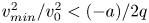 ${v^2_{min}}/{v^2_{0}}<({-a})/{2q}$, the mode is unstable, and as
  ${v^2_{min}}/{v^2_{0}}$ approaches
  $({-a})/{2q}$ from below, the wavenumber goes to zero. As long as
  $v_0^2\geq 2 v_{min}^2$, all wavenumbers higher than
  $\tilde {k}^2_<$ will be unstable. These thresholds are important for distinguishing regions of parameter space by the nature of their modes – periodic/exponentially growing and stable/unstable – as summarized in table 2.
Table 2. Types of solutions for various values of the parameters, assuming real  $a$,
$a$,  $q$. This article focuses on the cases with
  $k^2>0$ and
  $a<0$. Modes in columns shaded grey have imaginary wavenumber and are unphysical for the system we consider.

For a 2 $\ \textrm {cm}$ wavelength, the Earth's gravitational field sets the acoustic amplitude threshold at
 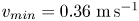 $v_{min}=0.36\ \textrm {m}\,\textrm {s}^{-1}$ (Mach number of approximately 0.001 in air) before convection sets in. This low Mach number validates the use of the linear acoustics regime in the derivation of (2.1). Far beyond threshold, the limiting value of the growth rate is
  $\sqrt {-b k_0^2 v_0^2/2}$. Calculating this value for
  $b=2\times 10^{-4}$, which corresponds to a 1
 $\ \textrm {K}$ temperature difference over the
  $2\ \textrm {cm}$ wavelength at room temperature, and the acoustic amplitudes of
  $20\ \textrm {m}\,\textrm {s}^{-1}$ measured in the experiment gives a growth rate of
  $\sigma =63\ \textrm {Hz}$. With more extreme parameters characteristic of the conditions inside the spherical plasma bulb experiment shown in figures 2 and 4, the growth rate can be
  $>10^5\ \textrm {Hz}$.
4.4. Finite viscosity
In § 4.3, we learned that the inertially limited growth rate is larger for short wavelengths (large  $-a$), but once the wavelength becomes shorter than a certain value the growth rate saturates. Viscosity must be included to determine a preferred, finite wavenumber. When combined with the growth rate, a new length scale – the viscous penetration depth – is introduced to the problem, adding more physical regimes. Examination of (4.13), reproduced here for convenience,
 \begin{equation} 0={-}\frac{1}{\tilde{\sigma}}\frac{\partial^4 w}{\partial \zeta^4} + \left(1+\frac{2\tilde{k}^2}{\tilde{\sigma}}\right)\frac{\partial^2 w}{\partial \zeta^2}-\tilde{k}^2\left(1+\frac{\tilde{k}^2}{\tilde{\sigma}}+\frac{\tilde{g}}{\tilde{\sigma}^2}+\frac{2\gamma^2}{\tilde{\sigma}^2} \cos2\zeta \right)w \end{equation}
lends more insight into the problem. The inertial, gravitational and driving terms discussed in § 4.3 are immediately identifiable. The additional terms due to viscosity come in two forms: (i) proportional to  $1/\tilde {\sigma }=\nu k_0^2/\sigma$, which is the square of the ratio of the viscous penetration depth to the plate separation (or acoustic wavelength), and (ii) proportional to
  $\tilde {k}^2/\tilde {\sigma }=\nu k^2/\sigma$, which is the square of the ratio of the viscous penetration depth to the instability wavelength. The fourth derivative is only appreciable for slow enough growth rates that the viscous penetration depth becomes comparable to the plate separation. On the other hand, the
  $\tilde {k}^2/\tilde {\sigma }$ terms appear as an increased resistance at high wavenumber.
Equation (4.24) is a fourth-order ordinary differential equation with variable coefficients, and is quadratic in its eigenvalue. We obtain approximate numerical solutions by linearizing in three limits and using a linear eigenvalue solver. The linearized forms of (4.24) are:
(i) for
 $\tilde {k}^2\ll \tilde {\sigma }$ (penetration depth small compared to the instability wavelength)
(4.25)\begin{equation} 0={-}\tilde{\sigma}\frac{\partial^4 w}{\partial \zeta^4} + \tilde{\sigma}^2\frac{\partial^2 w}{\partial \zeta^2}-\tilde{k}^2(\tilde{\sigma}^2+\tilde{g}+2\gamma^2 \cos2\zeta )w; \end{equation}
$\tilde {k}^2\ll \tilde {\sigma }$ (penetration depth small compared to the instability wavelength)
(4.25)\begin{equation} 0={-}\tilde{\sigma}\frac{\partial^4 w}{\partial \zeta^4} + \tilde{\sigma}^2\frac{\partial^2 w}{\partial \zeta^2}-\tilde{k}^2(\tilde{\sigma}^2+\tilde{g}+2\gamma^2 \cos2\zeta )w; \end{equation}(ii) for
$\tilde {k}^2\gg \tilde {\sigma }$ (penetration depth large compared to the instability wavelength)
(4.26)\begin{equation} 0={-}\tilde{\sigma}\frac{\partial^4 w}{\partial \zeta^4} + 2\tilde{\sigma}\tilde{k}^2\frac{\partial^2 w}{\partial \zeta^2}-\tilde{k}^2(\tilde{\sigma}\tilde{k}^2+\tilde{g}+2\gamma^2 \cos2\zeta )w;\end{equation}(iii) for
$\tilde {k}^2=\tilde {\sigma }-\delta \tilde {\sigma }$, with ${\delta \tilde {\sigma }}/{\tilde {k}^2}\ll 1$ (penetration depth comparable to instability wavelength)
(4.27)In regime (i), we take the eigenvalue to be\begin{align} 0&={-}\tilde{k}^2\left(1+\frac{\delta\tilde{\sigma}}{\tilde{k}^2}\right)\frac{\partial^4 w}{\partial \zeta^4} + \tilde{k}^4\left(3+4\frac{\delta\tilde{\sigma}}{\tilde{k}^2}\right)\frac{\partial^2 w}{\partial \zeta^2}\nonumber\\ &\quad -\tilde{k}^2\left(\tilde{k}^4\left(2+3\frac{\delta\tilde{\sigma}}{\tilde{k}^2}\right)+\tilde{g}+2\gamma^2 \cos2\zeta \vphantom{\frac{\delta\tilde{\sigma}}{\tilde{k}^2}}\right)w. \end{align}$\widetilde {k^2}$ for parameters $\tilde {\sigma }$, $\tilde {g}$ and $\gamma$; in regime (ii) we take the eigenvalue to be $\tilde {\sigma }$ for parameters $\widetilde {k^2}$, $\tilde {g}$ and $\gamma$; and in regime (iii) we take the eigenvalue to be $\delta \tilde {\sigma }$ for parameters $\widetilde {k^2}$, $\tilde {g}$ and $\gamma$.


Dispersion diagrams of the three fastest growing modes are plotted in figure 8 for  $\tilde {g}=0$ and various
  $\gamma$. The regimes of validity of (4.25), (4.26) and (4.27) are determined by the line
  $\tilde {\sigma }=\tilde {k}^2$, which is indicated by the dashed line in the figures. Equation (4.25) is valid far to the left of the dashed line, (4.26) is valid far to the right and (4.27) is valid near the line. Figure 9(a) shows how the growth rate for the fastest growing mode increases with the acoustic drive
  $\gamma$. Solutions
  $w[\zeta ]$ are plotted in figure 10.

Figure 8. Growth rates of the three fastest growing modes for  $\tilde {g}=0$ and various values of
  $\gamma$ generated by linearizing equation (4.24) in three regimes and using a linear eigenvalue solver. The three regimes are distinguished by the
  $\tilde {\sigma }=\tilde {k}^2$ line (dashed line) as described in the text.

Figure 9. (a) Dispersion diagrams of the fastest growing mode for  $\tilde {g}=0$ and various values of
  $\gamma$. (b) Normalized growth rates for
  $\tilde {g}=0$, large
  $\gamma$ and
  $\tilde {k}^2\ll \tilde {\sigma }$ (solutions of (4.25)) compared to those in the zero-viscosity limit. The
  $\gamma =\infty$ curve is the zero-viscosity limit, and is the solution of (4.15) also plotted in figure 5(b). The deviation at low
  $\tilde {k}^2$ arises when the viscous penetration depth becomes comparable to the plate separation.

Figure 10. Solutions of (4.25), (4.26) and (4.27) for various values of the parameters with  $\tilde {g}=0$. The character of the solutions does not change dramatically over a broad range of parameters, with the main difference being the size of the viscous penetration depth near the boundaries that is determined by the growth rate. At the highest
  $\gamma$, the convection is better isolated in the bottom half of the volume.
At low  $\gamma$, the viscous penetration depth is larger than both the separation between plates and the instability wavelength, and there is only a competition between shear at the wall and shear in the bulk. For
  $\tilde {g}=0$, the wavenumbers with the highest growth rate for the three fastest modes are
  $\tilde {k}^2=3.98, 15.8,$ and
  $36.3$ respectively, and their mode structure is plotted in figure 11.

Figure 11. The two fastest growing modes for  $\tilde {g}=0$,
  $\tilde {\gamma }=1$,
  $b=0.1$ at their fastest growing wavenumbers
  $\tilde {k}^2=4$ and 16.
As discussed in § 4.3, gravity stabilizes the fluid and sets a minimum acoustic amplitude for the instability to form. The threshold is simply determined by the condition for the effective gravity,  $\hat {z}\boldsymbol {\cdot }(\boldsymbol {g}+\boldsymbol {\nabla }\langle v_1^2\rangle /2)$ to change sign at some location in the system, and viscosity does not modify that condition. In terms of the dimensionless quantities, the threshold is
  $2\gamma ^2>\tilde {g}$. Viscosity does, however, unevenly modify the growth rate of the modes and consequently plays a role in selecting which mode grows fastest. Figure 12 shows the effect of increasing gravity on the growth rate. In addition to decreasing the growth rate, the peak of the growth rate curves moves towards higher wavenumbers. Figure 13 shows its effect on
  $w[\zeta ]$. The convective flow becomes more confined to the centre of the bottom half of the volume, around
  $\zeta =-0.5{\rm \pi}$, which is a consequence of narrowing the region where the effective gravity reverses sign.

Figure 12. Dispersion curves of the fastest growing mode for  $\gamma =0.3$ (a) and
  $\gamma =100$ (b) for various values of
  $\tilde {g}$. The modes are unstable when
  $2\gamma ^2>\tilde {g}$, and as
  $\tilde {g}$ approaches
  $2\gamma ^2$ the growth rate goes to zero while the peak of the growth rate curve shifts to higher wavenumber.

Figure 13. Solutions  $w[\zeta$] for various values of
  $\tilde {g}$ and
  $\gamma =0.3$ (a) or
  $\gamma =100$ (b). As the threshold
  $2\gamma ^2>\tilde {g}$ is approached, the width of the region where the sign of the effective gravity flips becomes narrower, restricting the convection to a smaller volume.
For large  $\gamma$ and
  $2\gamma ^2\gg \tilde {g}$,
  $\tilde {\sigma }$ scales with
  $\gamma$, but the un-normalized growth rate
  $\sigma$ saturates according to (4.18) (it is limited by inertia, not viscosity). Thus the solutions for large
  $\gamma$ and
  $\tilde {k}^2\ll \tilde {\sigma }$ (left of the dotted line) converge onto those found in the zero-viscosity limit (figure 5), as shown in figure 9(b). The deviation at low
  $\tilde {k}^2$ arises when the viscous penetration depth becomes comparable to the plate separation. At high
  $\tilde {k}^2$, the approximately constant growth rate found in the zero-viscosity limit extends up to where the
  $\tilde {k}^2\ll \tilde {\sigma }$ approximation breaks down, or when the viscous penetration depth becomes comparable to the instability wavelength. This ‘upper-bound’ wavenumber is,
 \begin{equation} \tilde{k}^2_{>}\simeq\tilde{\sigma}_{max}\simeq\sqrt{\frac{-b v_0^2}{2 \nu^2 k_0^2}-\frac{2bg}{\nu^2 k_0^3}}=\sqrt{2\gamma^2-\tilde{g}}\simeq\sqrt{2}\gamma, \end{equation}
which together with  $\tilde {k}^2_{<}$ of (4.20) determines a band of wavenumbers of approximately constant growth rate.
5. Multiple stability zones
One could imagine systems with multiple acoustic velocity antinodes between two planar boundaries forming a series of regions that alternate in stability, as determined by whether the density gradient in the initial state is parallel or antiparallel with the gradient in the time-averaged square of the acoustic velocity. Our approach can be extended to 2-D planar systems where the plate separation  $L$ is multiple acoustic half-wavelengths, i.e.
  $L=m {\rm \pi}/k_0$ for integer
  $m$, by applying the boundary conditions at a new location. For example, if there are three acoustic half-wavelengths between the plates (
 $m=3$) applying the zero velocity boundary conditions at
  $\zeta =-3{\rm \pi} /4$ and
  $\zeta =9{\rm \pi} /4$ will generate the new spectrum. To compare with the
  $m=1$ case studied in the previous sections, it will be useful to label the modes with indices (
 $m, p, q$), where
  $p\leq m$ indicates the instability zone number counted up from the bottom in which most of the flow field is contained, and
  $q$ indicates the number of extrema in
  $w_{m,p,q}(\zeta )$, divided by the number of convective regions (
 $m$). It is equivalent to the number of vortices in each instability zone. Thus the modes studied in § 4 are
  $(1,1,1)$,
  $(1,1,2)$,
  $(1,1,3)$, etc.
To get a sense of the additional physics involved, we investigate the  $m=3$ case for a limited set of parameters. Focusing on the
  $q=1$ modes, the growth rates are plotted in figure 14 for a few
  $\gamma$, and figure 15 displays the solutions
  $w_{3,p,1}$ and some flow fields. The single
  $q=1$ mode for
  $m=1$ splits into the three modes
  $(3,p,1)$ for
  $p=1,$
  $2$ or
  $3$ for
  $m=3$, with varying ratios of flow in each instability zone. One,
  $(p=1)$, is mainly confined to the lowest instability zone, and its growth rate is very similar to that when
  $m=1$. The other two,
  $p=2$ and
  $3$, have substantial amplitude in both other instability zones, and have similar growth rates that are faster than that of
  $p=1$. An important distinction is that the lowest instability zone is the only one with a boundary immediately adjacent to it, with the rest having fluid on both sizes. Thus the growth rate of the
  $p=1$ mode is substantially different than that for
  $p>1$ modes. When
  $\tilde {k}^2\gtrsim 1$, the growth rates of the
  $p>1$ modes converge, and when
  $\tilde {k}^2\gtrsim 10$ they converge with that of the
  $p=1$ mode as well.

Figure 14. Increasing the plate separation so that multiple acoustic antinodes (of number  $m$) fit between the plates introduces an additional unstable region per half-wavelength of separation. Each unstable region supports modes analogous to the ones that exist with only one unstable region, so each mode curve of figure 9 (when
  $m=1$), splits into
  $m$ curves equal in quantity to the number of unstable regions. The growth times of the
  $q=1$ modes (one vortex per instability zone) are plotted for
  $\gamma =1, 10, 100$. The single curve
  $(1,1,1)$ when
  $m=1$ (dashed) splits into three (solid) curves when
  $m=3$. The lowest of the three is the
  $p=1$ mode,
  $(3,1,1)$ where the convection is in the lowest unstable region (see figure 15), and lies directly on top of the
  $(1,1,1)$ curve. In the other two modes, the convection is mainly in the other two unstable regions (see figure 15).

Figure 15. Solutions  $w_{3,p,1}$ and flow fields for the
  $(3,p,1)$ modes. The lowest instability zone is the only one immediately adjacent to a boundary, and the mode with substantial amplitude near it
  $(p=1)$ has the slowest growth rate.
6. Conclusions
The pycnoclinic acoustic force acts to pull denser fluid towards velocity antinodes, and consequently stratified fluid in an acoustic field may be unstable if the density gradient is not parallel with the gradient in the time-averaged square of the acoustic velocity. In this article, we have solved for the unstable modes in a 2-D planar geometry, which have many of the same qualitative features as our experiment in a spherical plasma bulb.
In the 2-D planar system, gravity determines an acoustic amplitude threshold beyond which instability ensues,  $v_{min}=4|g|/k_0$. For a 2
 $\ \textrm {cm}$ wavelength on Earth,
  $v_{min}=0.36\ \textrm {m}\,\textrm {s}^{-1}$. Notably, the convection is isolated to only the part of the system where the density gradient is not parallel to the gradient in the time-averaged square of the acoustic velocity. For acoustic amplitudes much larger than threshold, the growth of small wavenumber modes is suppressed by inertia, while the growth of very high wavenumber modes is suppressed by viscosity in the bulk. There is a band of wavenumbers between the limits
  $\tilde {k}_<$ ((4.20)) and
  $\tilde {k}_>$ ((4.28)) with almost equivalent growth rate
  $\sigma =\sqrt {-b k_0^2 v_0^2/2}$.
A natural system that contains an internal division between stable and convecting regions is the Sun, and experiments based on versions of the convection described herein may be well suited to exploring that interface. Although differential rotation in the experiment has not yet been measured or otherwise verified, the presence of radially moving plumes in the equatorial plane with the bulk of the return flow at the mid latitudes suggests some form of differential rotation in order to conserve angular momentum. More terrestrial systems that may include forms of acousto-pycnoclinic convection are cryogenic pulse tubes and thermoacoustic engines (Radebaugh Reference Radebaugh1990; Backhaus & Swift Reference Backhaus and Swift2000), where it likely creates or suppresses (Swaminathan et al. Reference Swaminathan, Garrett, Poese and Smith2018) unwanted heat transport. The principles brought to light herein may be helpful in understanding it.
An application enabled by this work is the suppression of Rayleigh–Bénard convection with sound waves. If one imagines inverting the planar system considered here so that the hot plate was on the bottom and the cold plate on top, it would be very similar to the classic Rayleigh–Bénard problem and convection would occur naturally. Application of a sound wave above threshold would stabilize the bottom half of the system and suppress convection therein, but would also help drive convection in the top half. The net effect of the sound is to halve the characteristic length scale of the convection and also to increase the effective strength of gravity. Since thermal transport in the system is a function of the effective Rayleigh number, which is proportional to  $|g|L^3$, there will be a range of acoustic field amplitudes which will reduce the thermal transport. It is also of interest to consider how the heat transport will scale in the case where the sound creates multiple stability zones between the plates and transport will alternate between conduction and convection. In that case the effective Rayleigh number might be reduced substantially.
Applying an analogous theory to a spherical, rotating system is of interest. The Mach number in the spherical plasma convection experiment (Koulakis et al. Reference Koulakis, Pree, Thornton and Putterman2018c) can be larger than  $50{\times }$ the threshold set by gravity in a 2-D system of comparable wavelength. Rotation of the 15
 $\ \textrm {mm}$ radius sphere at
  ${\sim }50\ \textrm {Hz}$ generates a centrifugal force pointing cylindrically outwards that is
  ${\sim }150\times$ stronger than gravity, and might slow down or stabilize the convection at the equator. Combining experimental and theoretical studies of the interaction of spherically symmetric acoustic radiation pressure with rotation is a promising avenue of next generation convection research.
We are most excited about the prospects of having a terrestrial experiment to study Rayleigh–Bénard convection in a rotating, central force system. This is a rich problem which has been studied theoretically (Roberts Reference Roberts1968; Jones, Soward & Mussa Reference Jones, Soward and Mussa2000; Dormy et al. Reference Dormy, Soward, Jones, Jault and Cardin2004) and numerically (Hart, Glatzmaier & Toomre Reference Hart, Glatzmaier and Toomre1986b; Featherstone & Hindman Reference Featherstone and Hindman2016) for quite a while. Progress on the experimental front will require stabilization of the acoustic field in the plasma experiment, one method of which was studied theoretically by Pree, Putterman & Koulakis (Reference Pree, Putterman and Koulakis2019). Further theoretical exploration of the differences between acoustic ‘gravity’ and actual gravity, and in particular how well the former models the later, will be required to put such experiments on firmer ground. The analogy we have drawn herein applies when density differences over the system are small and the Boussinesq approximation holds. For systems with large density differences, the flow fields may have a significant divergence, and physical parameters such as the thermal conductivity and viscosity may vary with location. We posit that the physical consequences of these so-called non-Boussinesq effects (Zhang, Childress & Libchaber Reference Zhang, Childress and Libchaber1997; Sameen, Verzicco & Sreenivasan Reference Sameen, Verzicco and Sreenivasan2008) are fundamentally different between acoustic and true gravity and the analogy no longer holds. For example, one big complication that arises in the acoustic case with large density fluctuations, is that the motion of the fluctuations alters the acoustic field itself because the density appears in wave equation.
Acknowledgements
Inspiration for this manuscript was acquired through several in depth discussions with N. Featherstone and J. Aurnou which forced the authors to clarify the distinction between acoustic gravity and actual gravity. The breakthrough came during detailed conversations with G. Swift on the nature of acoustic forces on inhomogeneities and the resulting pressure and streaming flows. This work would not have been completed without their interest, engagement and encouragement.
Funding
This research was developed with funding from the Defense Advanced Research Projects Agency (DARPA D19AP00015). The views, opinions and/or findings expressed are those of the authors and should not be interpreted as representing the official views or policies of the Department of Defense or the U.S. Government. Approved for public release; distribution is unlimited. Initial interest in this work began while supported by the Air Force Office of Scientific Research under Award No. FA9550-16-1-0271.
Declaration of interests
The authors report no conflict of interest.


