3.1. Theoretical derivation

Turbulence has many degrees of freedom, which gives rise to a high-dimensional phase space. Directly studying turbulent dynamics in a high-dimensional phase space is difficult (if not impossible). In order to make progress, we must simplify the NS equation according to the specific flow under consideration.

The NS equation for RPCF reads

(3.1)\begin{equation} \frac{\textrm{D} u_i}{\textrm{D} t}={-}\frac{1}{\rho}\frac{\partial p}{\partial x_i}+\frac{1}{Re_w} \frac{\partial^2 u_i}{\partial x_k^2}-\epsilon_{i2k}\,Ro\,u_k, \end{equation}

where $u_i$ is the fluid velocity in the $i$th Cartesian direction, $\textrm {D}/\textrm {D}t$ is the total derivative and $i=1$, 2, 3 denote the streamwise, spanwise and wall-normal directions. We use $x$, $y$, $z$ interchangeably with $x_i$; $u$, $v$, $w$ interchangeably with $u_i$; and $\partial _i$ interchangeably with $\partial /\partial x_i$, $i=1$, 2, 3. Normalization is by half of the wall velocity difference $U_w$ and the half-channel height $h$. The bulk Reynolds number is $Re_w=U_wh/\nu$. In the main text, we present derivations for plane Couette flow. Derivations for TCF (which is concerned with surface curvature) are presented in appendix A.

First, we filter the NS equation in the streamwise direction at a scale $\sim O(h)$ to remove the small scales and focus on the large-scale roll cells. The filtered streamwise velocity equation reads

(3.2)\begin{equation} \frac{\textrm{D}\tilde{u}_1}{\textrm{D}t}={-}\frac{1}{\rho}\partial_1 \tilde{p}-\partial_j \tilde{T}_{1j} + \frac{1}{Re_w}\partial_j\partial_j \tilde{u}_1-Ro \tilde{u}_3, \end{equation}

where $\tilde {\cdot }$ denotes streamwise filtration and $\tilde {T}_{1j}$ is the turbulent stress. We define the filtered vorticity $\tilde {\omega }_i=\epsilon _{ijk}\partial _j \tilde {u}_k$. The streamwise vorticity equation reads

(3.3)\begin{equation} \frac{\textrm{D}\tilde{\omega}_1}{\textrm{D}t}=\tilde{\omega}_j\partial_j \tilde{u}_1-\epsilon_{1qi}\partial_q\partial_j\tilde{T}_{ij}+\frac{1}{Re_w}\partial_j\partial_j\tilde{\omega}_1+Ro\partial_2\tilde{u}_1. \end{equation}

For a spanwise RPCF that features multiple statistically stable states, the flow is approximately streamwise homogeneous, and we neglect the streamwise derivatives. To focus on the dynamics of the large-scale roll cells, we invoke the eddy viscosity model. It follows that the vortex stretching term $\tilde {\omega }_j\partial _j \tilde {u}_1$ is zero upon substitution of the vorticity, $\tilde {\omega }_j=\epsilon _{jpq}\partial _p \tilde {u}_q$. Hence, (3.2) and (3.3) lead to

(3.4)\begin{equation} \partial_t\tilde{u}_1+\tilde{u}_j\partial_j\tilde{u}_1=\partial_j\left[\left(\frac{1}{Re_w}+\nu_t\right)\partial_j\tilde{u}_1\right]-Ro \tilde{u}_3 \end{equation}

and

(3.5)\begin{equation} \partial_t\tilde{\omega}_1+\tilde{u}_j\partial_j\tilde{\omega}_1=\partial_j\left[\left(\frac{1}{Re_w}+\nu_t\right)\partial_j\tilde{\omega}_1\right]+Ro\partial_2\tilde{u}_1, \end{equation}

where $j=2,3$, $\nu _t$ is the eddy viscosity and $\partial _{jj}=\partial _{22}+\partial _{33}$.

Second, we define a streamfunction $\psi$ such that

(3.6)\begin{equation} \left.\begin{gathered} \tilde{u}_2=\partial_3\psi, \\ \tilde{u}_3={-}\partial_2\psi. \end{gathered}\right\}\end{equation}

It follows that $\tilde {\omega }_1=-\partial _j\partial _j\psi$. Plugging (3.6) into (3.4) and (3.5) leads to

(3.7)\begin{equation} \partial_t\tilde{u}_1 +\partial_2\tilde{u}_1\partial_3\psi-\partial_3\tilde{u}_1\partial_2\psi =\partial_j\left[\frac{1}{R}\partial_j\tilde{u}_1\right]+Ro\partial_2\psi \end{equation}

and

(3.8)\begin{equation} \partial_t\partial_j\partial_j\psi +\partial_2\partial_j\partial_j\psi\partial_3\psi-\partial_3\partial_j\partial_j\psi\partial_2\psi=\partial_j\left[\frac{1}{R}\partial_j\partial_q\partial_q \psi\right]-Ro\partial_2\tilde{u}_1. \end{equation}

In the above equations, we have invoked the effective Reynolds number $R=1/(1/Re_w+\nu _t)$ following Anderson (Reference Anderson2019). As the eddy viscosity is generally not a constant, invoking the effective Reynolds number is a crude approximation. Nonetheless, in this context, because the eddy viscosity in the bulk region of a spanwise rotating channel is in fact close to a constant (Yang et al. Reference Yang, Xia, Lee, Lv and Yuan2020a), invoking the effective Reynolds number here has a somewhat sounder physical basis.

Third, we project (3.7) and (3.8) onto a statistically stable state:

(3.9)\begin{equation} \left.\begin{gathered} \psi(x_2,x_3,t)=a(t)\alpha(x_2,x_3),\\ \tilde{u}_1(x_2,x_3,t)=b(t)\beta(x_2,x_3)+U(x_3), \end{gathered}\right\}\end{equation}

where $\alpha$ and $\beta$ represent roll cells of a given wavenumber and $U(x_3)$ is the mean flow. Here, we assume that the mean flow does not depend on a particular state. This assumption is consistent with the data and simplifies the analysis that follows. Relaxing this assumption leads to more involved mathematics but essentially the same conclusions, as shown in appendix B. Plugging (3.9) into (3.7) and (3.8) leads to

(3.10)\begin{equation} \beta \frac{\textrm{d}b}{\textrm{d}t}+ab\partial_2\beta\partial_3\alpha-ab\partial_3\beta \partial_2\alpha-a\partial_3U \partial_2\alpha =\frac{1}{R}b\partial_j\partial_j\beta+\frac{1}{R}\partial_3\partial_3U+Ro\,a\partial_2\alpha \end{equation}

and

(3.11)\begin{align} \partial_j\partial_j\alpha \frac{\textrm{d}a}{\textrm{d}t}+a^2(\partial_2\partial_j\partial_j\alpha\partial_3\alpha-\partial_3\partial_j\partial_j\alpha\partial_2\alpha) =\frac{1}{R}a\left[\partial_2^4\alpha+2\partial_2^2\partial_3^2\alpha+\partial_3^4\alpha\right]-Ro\,b\partial_2\beta. \end{align}

Equations (3.10) and (3.11) govern the dynamics of roll cells. In (3.10) and (3.11), we have left $\alpha$ and $\beta$ as generic functions of $y$ and $z$, and, importantly, we have retained nonlinearity.

Fourth, we need ansatzes for $\alpha$ and $\beta$ in order to advance. The DNS solution is by itself a good ansatz: it is a solution to the Reynolds-averaged NS equation, and it satisfies the no-slip condition. However, the use of DNS data necessarily involves numerical tools in the following derivations, and we will postpone the analysis to appendix C. Here, we use the following analytical ansatz to approximate the multiple states:

(3.12)\begin{equation} \left.\begin{gathered} \alpha={-}\sin\left(\frac{\rm \pi}{2}ky\right)\cos\left(\frac{\rm \pi}{2}z\right),\\ \beta={-}\cos\left(\frac{\rm \pi}{2}ky\right)\left[1-\cos\left({\rm \pi} z\right)\right]. \end{gathered}\right\}\end{equation}

The ansatz in (3.12) does not satisfy the no-slip condition at $z/h=\pm 1$. This is in fact a common practice analysis (Chandra & Verma Reference Chandra and Verma2013; Wagner & Shishkina Reference Wagner and Shishkina2013; Chong et al. Reference Chong, Wagner, Kaczorowski, Shishkina and Xia2018). For example, Anderson (Reference Anderson2019) applied truncated Galerkin projection to study the dynamics of the secondary flows above spanwise heterogeneous surface roughness, and the ansatz used in his work does not satisfy the no-slip condition. Also, when studying large-scale circulation reversal in Rayleigh–Bénard flows, Chen et al. (Reference Chen, Huang, Xia and Xi2019) applied truncated Galerkin projection and projected the instantaneous flow field onto a few Fourier modes, and these modes do not satisfy the no-slip condition on wall boundaries. In general, when applying truncated Galerkin projection, the idea is to focus on the bulk flow behaviour. 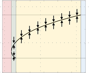Figure 3 shows the ansatz for $k=3/{\rm \pi}$, which corresponds to $R3$. As we can see from figure 3, the ansatz compares well with the data, i.e. figure 1(b). Quantitatively, our analytical ansatz (which contains but only one Fourier mode) contains about 55 % of the energy in $\tilde {u}$ and about 90 % of the energy in $\tilde {v}$ and $\tilde {w}$. The next most energetic Fourier mode contains about 7 % of the energy in $\tilde {u}$ and 1 % of the energy in $\tilde {v}$ and $\tilde {w}$. For $R2$, our analytical ansatz contains about 60 % of the energy in $\tilde {u}$ and about 85 % of the energy in $\tilde {v}$ and $\tilde {w}$. The next most energetic Fourier mode contains about 7 % of the energy in $\tilde {u}$ and about 4 % of the energy in $\tilde {v}$ and $\tilde {w}$. One can, of course, obtain more realistic ansatzes by including additional terms in (3.12). Figure 4 shows the energy contained in the ansatzes as we include more Fourier modes. As one would expect, accuracy comes at the price of brevity. In appendix C, we use the DNS solution as our ansatz, and we show that our conclusions are not affected.

Figure 3. Equation (3.12) with $k=3/{\rm \pi}$. Contours are for $u$ and vectors are for $v$ and $w$. Again, the exact contour values are not important.

Figure 4. The energy contained in the ansatz as a function of $n$, where $n$ is the number of terms in the ansatz. The thick lines are for $u$. The thin lines are for $\psi$. The dashed lines are for $R2$. The solid lines are for $R3$.

3.2. Dynamics of the stable states

Before we proceed with our derivation, we take a close look at the flow dynamics near the two stable states in $R2$ and $R3$ so that we have in mind what to expect. Equations (3.10) and (3.11) map the roll cell dynamics to two variables: $a$ and $b$. We define the projection operator as

(3.13)\begin{equation} \int_0^{L_y}\int_{{-}1}^{1} f\cdot \alpha \,\textrm{d}z \,{\textrm{d} y}, \end{equation}

where we project $f$ onto $\alpha$. We project the DNS data on the ansatzes in (3.12) and get $a$ and $b$. The two values can be understood as containing both the real and the imaginary parts of the corresponding Fourier mode. In figure 5(a), we plot the trajectories of $R2$ and $R3$ in the phase space of $a$ and $b$. The two trajectories circle around their time means. Because the two DNSs have reached statistically stationary states, $a$ and $b$ do not decay or increase. For comparison, in figure 5(b), we plot the trajectory of the shell model, an ergodic model for energy cascade, in the subphase space of two Fourier modes. The integral length of the corresponding isotropic flow is $L$. The two Fourier modes correspond to the length scales of $L/2$ and $L/8$ (relatively large-scale modes). Details of the data in figure 5(b) are presented in appendix D. Comparing figures 5(a) and 5(b), the trajectory in figure 5(b) visits a large area in the phase space and is easily ergodic, but the two trajectories in figure 5(a) are confined in two small regions, and the two regions do not overlap, thereby leading to two statistically stable states.

Figure 5. (a) Trajectories of $R2$ and $R3$ in the phase space of $a$ and $b$. (b) Trajectory of the shell model for isotropic turbulence in the subphase space of two Fourier modes $\hat {u}_2$ and $\hat {u}_3$. The $x$ and $y$ axes in both panels span two decades.

Figure 6 shows a zoom-in view of the trajectories in the phase space of $a^\prime$ and $b^\prime$, where the superscript $\prime$ denotes temporal fluctuations. Limit-cycle-like trajectories are found in both $R2$ and $R3$. The time elapse of the data is $1000h/U_w$ (Xia et al. Reference Xia, Shi, Cai, Wan and Chen2018). Xia et al. could not rule out the possibility of state exchange because it was not clear how 1000$h/U_w$ compares to the turnover time of a roll cell. For example, if the eddy turnover time of a roll cell is 10$h/U_w$, the simulation time 1000$h/U_w$ would be sufficient to rule out the possibility of state exchange, but if the eddy turnover of a roll cell is $10\,000 h/U_w$, the simulation time $1000h/U_w$ would not be sufficient. Figure 6 addresses the above question. The time it takes to do a circle in the phase space is a good approximation of a roll cell's turnover time. Here, the flow is not able to escape after many cycles, and therefore we can safely conclude that $R2$ and $R3$ are stable multiple states. For reasons that will be clear in the next subsection, we fit $\textrm {d}a^\prime /\textrm {d}t$ and $\textrm {d}b^\prime /\textrm {d}t$ to the linear dynamics $c_1a^\prime +c_2b^\prime$, where $c_1$ and $c_2$ are constants. In figures 7 and 8, the data are compared to the linear dynamics, and the two are remarkably similar, suggesting that the flow near the two stable states is governed by linear dynamics. Ergodicity relies on sufficiently large fluctuations, and in a turbulent flow system, large fluctuations are often results of nonlinear interactions. The fact that the evolution of $a^\prime$ and $b^\prime$ follows linear dynamics explains, from a phenomenological standpoint, why the flow is trapped within a stable state. The challenge remains as to whether we could theoretically show that $a$ and $b$ follow linear dynamics.

Figure 6. Zoomed view of the trajectories of (a) $R2$ and (b) $R3$ in the phase space of $a^\prime$ and $b^\prime$.

Figure 7. The time evolution of (a) $a^\prime$ and (b) $b^\prime$ in $R2$ and fits to linear dynamics.

Figure 8. The time evolution of (a) $a^\prime$ and (b) $b^\prime$ in $R3$ and fits to linear dynamics.

3.3. Truncated Galerkin projection and bifurcation analysis

We proceed with our derivation. In § 3.1, we were at step four. In § 3.2, we saw that the data suggest linear dynamics near a stable state. In this section, we see if our derivation gives rise to the observed linear dynamics. The fifth step is to plug (3.12) into (3.10) and (3.11) and project the two equations onto the ansatzes in (3.12). Projection is defined in (3.13). After some (long) algebra, we arrive at

(3.14)\begin{equation} \frac{\textrm{d}b}{\textrm{d}t}=\left[\frac{4k}{9}Ro+\frac{k{\rm \pi}}{3}\int_{{-}1}^1\sin^2\left(\frac{\rm \pi}{2}z\right) \cos\left(\frac{\rm \pi}{2}z\right)\frac{\textrm{d}U}{\textrm{d}z} \textrm{d}z\right]a -\left(k^2+\frac{4}{3}\right)\frac{1}{R}\left(\frac{\rm \pi}{2}\right)^2b \end{equation}

and

(3.15)\begin{equation} \frac{\textrm{d}a}{\textrm{d}t}={-}\frac{1}{R}(k^2+1)({\rm \pi}/2)^2a -\frac{4}{3}\frac{k}{k^2+1}Ro({\rm \pi}/2)^{{-}2}b, \end{equation}

which is indeed linear dynamics. In arriving at the above two equations, we invoke $\sin ({\rm \pi} /2kL_y)=0$ since there can only be integer pairs of roll cells in the domain. It is worth noting that truncated Galerkin projection does not preclude nonlinearity. The integral in (3.14) is

(3.16)\begin{align} \int_{{-}1}^1\sin^2\left(\frac{\rm \pi}{2}z\right)\cos\left(\frac{\rm \pi}{2}z\right)\frac{\textrm{d}U}{\textrm{d}z} \textrm{d}z={-}\int_{{-}1}^1 U\frac{\rm \pi}{2} \sin\left(\frac{\rm \pi}{2}z\right)\left[2-3\sin^2\left(\frac{\rm \pi}{2}z\right)\right]\textrm{d}z \approx 0.27 \end{align}

for both $R2$ and $R3$. Although it is somewhat trivial, we note that according to (3.16), the integral is concerned with $U$ not its derivative.

We are now at the last step. Sixth, we conduct bifurcation analysis of the ordinary differential equations in (3.14) and (3.15). If multiple statistically stable states exist, $\textrm {d}a/\textrm {d}t=0$ and $\textrm {d}b/\textrm {d}t=0$ must have multiple non-trivial solutions. Hence, if multiple states exist, the eigenvalues of the ordinary differential equations in (3.14) and (3.15) must be such that

(3.17)\begin{equation} \lambda_{1,2}=0, \end{equation}

for non-trivial $a$ and $b$. This necessarily leads to

(3.18a,b)\begin{equation} (k^2+1)^2(k^2+4/3)-Ck^2=0,\quad C\approx{-} \left(0.039 Ro^2+0.025 Ro\right)R^2. \end{equation}

Equation (3.18a,b) is a cubic equation of $k^2$ (note that $Ro<0$ and $C>0$). For certain $C$, i.e. for certain flow condition, there are two physically viable roots:

(3.19)\begin{equation} \left.\begin{gathered} k_1^2=h^{1/3} + gh^{{-}1/3} - 10/9,\\ k_2^2={-}\textrm{i}\sqrt{3/4}\times( h^{1/3}- gh^{{-}1/3}) -1/2\times(h^{1/3} + gh^{{-}1/3})-10/9, \end{gathered}\right\} \end{equation}

where $f=5C/9+1/729$, $g=C/3+1/81$, $h=(\,f^2 - g^3)^{1/2} - f$, $\textrm {i}=\sqrt {-1}$, $\textrm {i}^{1/3}=\exp (\textrm {i}\cdot {\rm \pi}/6)$, $(-\textrm {i})^{1/3}= \exp (-\textrm {i}\cdot {\rm \pi}/6)$. Here, $k_2^2$ is real and is positive despite the appearance of the unit imaginary number $\textrm {i}$. Hydrodynamic stability does not allow for very slim or very fat roll cells (Drazin & Reid Reference Drazin and Reid2004). Determining the limits of roll cell aspect ratio falls out of the scope of this paper. Here, we arbitrarily cut off at $k=0.5$ and $k=2$, constraining that the roll cell heights to be no more than twice their widths and no less than half their widths. Figure 9 shows the bifurcation diagram, where we plot $k_1$ and $k_2$ as a function of $C$. We conclude our derivation here.

Figure 9. Bifurcation diagram. According to (3.18a,b), $C\approx -(0.039 Ro^2+0.025 Ro)R^2$. For the condition considered here, i.e. near $Ro=-0.2$, $C$ is an increasing function of the rotation speed $|Ro|$. We explain the arrows in § 4.1.

Before we proceed to predictions, we make two observations. First, truncated Galerkin projection preserves nonlinearity in the equation; however, the application of truncated Galerkin projection to this particular problem leads to linear dynamics. Second, (3.18a,b) is, strictly speaking, a sextic polynomial, which, in principle, has six roots. Nonetheless, it turns out that if one regards $k^2$ as the unknown, the equation reduces to a cubic one; and it also happens that one of the three roots of the cubic equation is always negative, leaving us only two physically viable roots.

4.1. Multiple states in an infinitely large domain

According to figure 9, for small values of $Ro$, the flow is in the red zone, and there is no physically viable root to (3.18a,b). It follows that, for a non-rotating plane Couette flow, multiple states that feature roll cells with different wavenumbers are not possible. For a flow that is in the green zone, i.e. for a moderate rotation number, (3.18a,b) has two roots between 0.5 and 2, leading to multiple states. This is evidenced by the multiple states in Xia et al. (Reference Xia, Shi, Cai, Wan and Chen2018). In the yellow zone, i.e. at high rotation speeds, (3.18a,b) has one root between 0.5 and 2. This means that while roll cells could still be found, they could only be found at one wavenumber. The existence of this regime is confirmed in Huang et al. (Reference Huang, Xia, Wan, Shi and Chen2019a): the authors increased $Ro$ from a small value to $Ro=0.5$ and found that the spanwise domain always contains four roll cells irrespective of the initial condition (i.e. there is only one stable state). Last, in the blue zone, i.e. at high rotation speeds, (3.18a,b) does not have a root between 0.5 and 2, and no roll cells could be found. The existence of this regime is also confirmed in Huang et al. (Reference Huang, Xia, Wan, Shi and Chen2019a): the authors increased the rotation speed to 0.6, and the flow could no longer sustain the roll cells. For $C$ that gives rise to multiple states, e.g. $C=9$, we plot the residual of the cubic equation (3.18a,b) in figure 10. The two statistically stable states, denoted as $k_1'$ and $k_2'$, yield 0. The residual measures the distance of a state from the equilibrium and therefore can be interpreted as a measure of the energy level. From figure 10, we can conclude that the large energy barrier between the two stable states locks the flow at one state, leading to non-ergodicity. The system would have been ergodic if the energy barrier is low or if the flow has enough energy to go from one state to the other. Figure 10 also has implications on the flow dynamics. For instance, if the flow is at $k=0.7$, i.e. a high-energy state, it will migrate to $k_1'$, i.e. a low-energy state. Visualizing the migration of every state in the $k$ space leads to the phase lines in figure 10, and visualizing these phase lines at all $C$ values leads to the arrows in figure 9.

Figure 10. Residual of (3.18a,b) for $C=9$. States $k_1'$ and $k_2'$ correspond to two states that yield 0 residual.

4.2. Multiple states in a finite domain

A finite domain admits only a few discrete wavenumbers. For a domain that extends $L_y=4{\rm \pi}$ in the spanwise direction, the wavenumber $k$ can only take values $1/{\rm \pi}$, $2/{\rm \pi}$, $3/{\rm \pi} ,\ldots n/{\rm \pi}$, where $n$ is an integer. Xia et al. (Reference Xia, Shi, Cai, Wan and Chen2018) observed bistability for $k=2/{\rm \pi}$ and $k=3/{\rm \pi}$. However, according to (3.18a,b), the two wavenumbers $k=2/{\rm \pi}$ and $3/{\rm \pi}$ correspond to two different values of $C$, i.e. $C_1$ and $C_2$. Because of this, according to figure 9, bistability of $k=2/{\rm \pi}$ and $3/{\rm \pi}$ would not be possible at a given flow condition (for a given $C$) in an infinite domain. In the following, we explain why bistability of $k=2/{\rm \pi}$ and $3/{\rm \pi}$ is possible in a finite domain of size $L_y=4{\rm \pi}$.

First, we pick two flow conditions, i.e. two $C$ values, $C'$ and $C''$, such that $C_1<C'<C''<C_2$. Figure 11(b) plots the energy of all possible states, i.e. $k$, for the two conditions $C'$ and $C''$. For an infinite domain, condition $C'$ will result in bistability at $s_1'$ and $s_2'$ and condition $C''$ will result in bistability at $s_1''$ and $s_2''$. However, for a domain of size $L_y=4{\rm \pi}$ and at the condition $C'$, $k$ takes values of $1/{\rm \pi}$, $2/{\rm \pi}$, $3/{\rm \pi} ,\ldots n/{\rm \pi}$ only. Among those values, $k=2/{\rm \pi}$ and $k=3/{\rm \pi}$ are at the lowest energy. Now, supposing the flow is at state $k=2/{\rm \pi}$, the energy barriers (the bumps in figure 11b) will keep the flow at $k=2/{\rm \pi}$; and if the flow is at state $k=3/{\rm \pi}$, the energy barriers will keep the flow at $k=3/{\rm \pi}$: making bistability of $k=2/{\rm \pi}$ and $k=3/{\rm \pi}$ possible at both conditions $C'$ and $C''$. This explains why $R2$ and $R3$ can be observed for a range of rotation numbers in a finite domain (Huang et al. Reference Huang, Xia, Wan, Shi and Chen2019a) and in general why the same multiple states can be observed within a range of flow conditions.

Figure 11. (a) States $R2$ ($k=2/{\rm \pi}$) and $R3$ ($k=3/{\rm \pi}$) and the corresponding $C$ values. State $R2$ corresponds to $C_1$ and $R3$ corresponds to $C_2$. Here, $C_1<C'<C''<C_2$. (b) Residual/energy for $C'$ and $C''$. Here $s_1'$, $s_2'$ are at $\textrm {res}=0$ for $C'$; $s_1''$, $s_2''$ are at $\textrm {res}=0$ for $C''$.

To elaborate, whether a state is statistically stable depends on whether the flow can migrate to a lower-energy state. A state will be statistically unstable if the flow can migrate to a lower-energy state, and a state will be statistically stable if the flow cannot migrate to a lower-energy state. A domain of size $L_z=4{\rm \pi}$ admits $k=1/{\rm \pi}$, $2/{\rm \pi} ,\ldots , n/{\rm \pi}$, where $n$ is an integer. All these states have a residual. Among these states, the two states $k=2/{\rm \pi}$ and $k=3/{\rm \pi}$ have the smallest residual, i.e. lowest energy. Because the two states cannot migrate from one to the other (due to the energy barrier) and because other states are at higher energy levels, the two states $k=2/{\rm \pi}$ and $k=3/{\rm \pi}$ are statistically stable, leading to bistability of these two states in a finite domain. Following the above discussion, we can now more precisely define ‘bistability’. Bistability does not necessarily refer to two states that have 0 residual; it refers to two states that do not migrate from one to the other nor migrate to other states.