


1 Introduction
Numerous natural systems contain narrow spaces that enable liquid transport, such as porous media (e.g. Wang & Cheng Reference Wang and Cheng1996). This behaviour, called capillary action, occurs because of the combination of surface tension and adhesive forces between liquid and solid. A typical example is the rise of a liquid in a capillary tube vertically positioned in an infinite liquid. From the aspect of statics, previous studies have been conducted to examine the shapes of equilibrium menisci dating back to the nineteenth century (Young Reference Young1805). It is known that the meniscus in a uniform circular tube can be uniquely determined by the contact angle and the tube radius. However, a non-uniform circular tube (i.e. an axisymmetric tube with a variable radius) may admit two or more equilibrium menisci (e.g. Finn Reference Finn1988; Tsori Reference Tsori2006). Except in a few cases, the uniqueness of menisci cannot always be expected (Finn Reference Finn1988).
Motivated by the non-uniqueness of menisci, an axisymmetric container (called the exotic container) which permits an entire continuum of equilibrium menisci was proposed and studied theoretically (Gulliver & Hildebrandt Reference Gulliver and Hildebrandt1986; Finn Reference Finn1988; Concus & Finn Reference Concus and Finn1989, Reference Concus and Finn1991). The exotic container is determined mathematically so that all the menisci have the same potential energy and bound the same volume of liquid. However, these axisymmetric menisci turn out to be unstable (i.e. none of them is a local minimizer of energy) (Finn Reference Finn1988; Concus & Finn Reference Concus and Finn1989; Wente Reference Wente1999), which leads to the prediction that there are non-axisymmetric menisci with a local minimum of energy in the exotic container. However, there is at present no known way to determine the non-axisymmetric menisci theoretically in the exotic container. Using the Surface Evolver software (Brakke Reference Brakke1992), the non-axisymmetric menisci were found numerically by Callahan, Concus & Finn (Reference Callahan, Concus, Finn and Taylor1991). Results showed that there are three distinct non-axisymmetric menisci in the exotic container. However, only two non-axisymmetric menisci were observed experimentally (Concus, Finn & Weislogel Reference Concus, Finn and Weislogel1992, Reference Concus, Finn and Weislogel1999). The loss of axisymmetry (i.e. the non-axisymmetric instability) is not an exclusive phenomenon for the exotic container. Non-axisymmetric instability can occur even if conditions for an exotic container are not entirely met (Concus et al. Reference Concus, Finn and Weislogel1999) and can also be observed for a liquid bridge when the Steiner limit is exceeded (Gillette & Dyson Reference Gillette and Dyson1972; Russo & Steen Reference Russo and Steen1986; Slobozhanin, Alexander & Resnick Reference Slobozhanin, Alexander and Resnick1997). Though the non-axisymmetric menisci, in general, cannot be determined mathematically, the stability analysis of menisci can allow one to obtain the critical conditions for the onset of non-axisymmetric instability. A comprehensive review of the stability of menisci has been presented by Bostwick & Steen (Reference Bostwick and Steen2015).
Inspired by the exotic container, Wente (Reference Wente2011) extended the ‘exotic’ property to a capillary tube and proposed a non-uniform circular tube, called the exotic capillary tube (ECT), vertically positioned in an infinite liquid which permits an entire continuum of equilibrium menisci. Following Wente (Reference Wente2011), Zhang & Zhou (Reference Zhang and Zhou2020) investigated the interior, exterior and planar cases of ECTs together (collectively called the exotic cylinder), and then examined their stabilities by the method of Slobozhanin & Alexander (Reference Slobozhanin and Alexander2003). Results showed that each of the menisci for the exotic cylinder has the smallest eigenvalue  $\unicode[STIX]{x1D706}_{01}=0$ to axisymmetric perturbations and the menisci are stable, in contrast to the case of the exotic container. This is because the stability is sensitive to the constraint on the liquid. The eigenvalue
  $\unicode[STIX]{x1D706}$ is associated with the second variation of energy and
  $\unicode[STIX]{x1D706}<0$ corresponds to instability. For the exotic containers, only volume-preserving variations (called volume disturbances) of the interface are allowed because there is a volume constraint. However, for the exotic cylinders, there is no volume constraint restricting the variations (called pressure disturbances). For an axisymmetric problem, both pressure and volume disturbances consist of axisymmetric perturbations and non-axisymmetric perturbations, where non-axisymmetric perturbations satisfy the volume constraint automatically (i.e. no added volume constraint is enforced on non-axisymmetric perturbations even for the constrained problem) (Myshkis et al. Reference Myshkis, Babskii, Kopachevskii, Slobozhanin, Tyuptsov and Wadhwa1987).
Then, we discuss why the axisymmetric menisci in the exotic containers are unstable to non-axisymmetric perturbations while the axisymmetric menisci in the exotic cylinders are stable. The ‘exotic’ property indicates that the axisymmetric menisci have the smallest eigenvalue  $\unicode[STIX]{x1D706}_{01}=0$ to axisymmetric perturbations for the exotic containers and the exotic cylinders (see Wente Reference Wente1999; Zhang & Zhou Reference Zhang and Zhou2020). Myshkis et al. (Reference Myshkis, Babskii, Kopachevskii, Slobozhanin, Tyuptsov and Wadhwa1987) have shown that for an unconstrained axisymmetric problem one has
  $\unicode[STIX]{x1D706}_{01}<\unicode[STIX]{x1D706}_{11}$, where
  $\unicode[STIX]{x1D706}_{11}$ is the smallest eigenvalue to non-axisymmetric perturbations, which means that the unconstrained axisymmetric meniscus to axisymmetric perturbations is less stable than to non-axisymmetric perturbations. Thus, the unconstrained axisymmetric menisci for the exotic cylinder are stable and have the smallest eigenvalue
  $\unicode[STIX]{x1D706}_{01}=0$ to pressure disturbances. For a constrained axisymmetric problem,
  $\min (\unicode[STIX]{x1D706}_{01},\unicode[STIX]{x1D706}_{11})$ is, in general, the smallest eigenvalue, and
  $\unicode[STIX]{x1D706}_{11}$ is the smallest eigenvalue in the case of simply connected menisci with Bond number
  $Bo>0$ (Myshkis et al. Reference Myshkis, Babskii, Kopachevskii, Slobozhanin, Tyuptsov and Wadhwa1987). Then we have
  $\unicode[STIX]{x1D706}_{11}<\unicode[STIX]{x1D706}_{01}=0$ for the exotic container, and therefore the menisci are unstable to non-axisymmetric perturbations. This conclusion was also drawn by Wente (Reference Wente1999) by examining the second variation of energy of the planar meniscus in the exotic container to all gravity levels. It was found that the infimum of the second variation of energy is less than zero. This can also be explained in that the axisymmetric planar menisci (which are assumed to exist in the exotic container) always have the relations
  $\unicode[STIX]{x1D706}_{01}>\unicode[STIX]{x1D706}_{11}$ for all values of the Bond number (see Myshkis et al. Reference Myshkis, Babskii, Kopachevskii, Slobozhanin, Tyuptsov and Wadhwa1987, pp. 140–143) and
  $\unicode[STIX]{x1D706}_{01}=0$ due to the ‘exotic’ property.

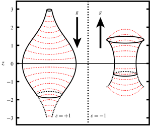
Figure 1. Profile of a meniscus meeting a solid at a contact angle  $\unicode[STIX]{x1D703}$ under gravity
  $g$. There are two directions of gravity: the downward and upward directions corresponding to positive loads
  $\unicode[STIX]{x1D700}=+1$ and negative loads
  $\unicode[STIX]{x1D700}=-1$, respectively. The meniscus is simply connected when the meniscus touches the axis of symmetry
  $r=0$. The case of an unconstrained liquid is considered and the water line is fixed at
  $z=0$ so that the pressure difference
  $\unicode[STIX]{x0394}p=-\unicode[STIX]{x1D700}z$.
The ECTs discussed above studied by Wente (Reference Wente2011) and Zhang & Zhou (Reference Zhang and Zhou2020) need to be vertically positioned correctly in an infinite liquid under positive loads (gravity down into the liquid) to have the ‘exotic’ property. To ensure the ECT is in contact with the infinite liquid, there must be an axisymmetric planar meniscus in the ECT. For negative loads, to our knowledge, the infinite liquid cannot be stable, though the corresponding ECT shapes can be determined mathematically. To make the ECTs under negative loads physically meaningful, we set an appropriate constant pressure at the inlet of the ECT (called a general ECT) instead of placing the ECT in an infinite liquid even though the above two considerations are in a sense the same mathematically. Thus, there will not necessarily be an axisymmetric planar meniscus in the general ECT and the general ECT shapes can be determined under positive and negative loads. Meanwhile, the stability analysis of axisymmetric menisci in ECTs can be also extended to the case of negative loads.
2 Theory
We describe the configuration of an unconstrained axisymmetric liquid partially wetting a solid using the notation shown in figure 1. By introducing cylindrical coordinates  $(r,z)$ with the origin located at the water line,
  $r$ is the radius from the axis of symmetry and
  $z$ is the height of the meniscus from the water line. The meniscus profile is represented by the parameterized curve
  $(r(s),z(s))$ by the introduction of its arc length
  $s$. We scale all lengths by the capillary length
  $l=\sqrt{\unicode[STIX]{x1D70E}/\unicode[STIX]{x1D70C}g}$, curvature by
  $l^{-1}$ and pressure by
  $\unicode[STIX]{x1D70C}gl$, where
  $\unicode[STIX]{x1D70E}$ is the surface tension of the interface,
  $\unicode[STIX]{x1D70C}$ is the density difference between the two fluids and
  $g$ is the gravitational acceleration.
2.1 Family of solution curves
As shown in figure 1, there are two directions of gravity for the configuration: the downward and upward directions corresponding to positive loads  $\unicode[STIX]{x1D700}=+1$ and negative loads
  $\unicode[STIX]{x1D700}=-1$, respectively. It is well known that the profile of the equilibrium meniscus is governed by the Young–Laplace equation, which can be expressed in parametric form (see e.g. Huh & Scriven Reference Huh and Scriven1969; Boucher & Evans Reference Boucher and Evans1975; Finn Reference Finn1986):
 $$\begin{eqnarray}\frac{\text{d}r}{\text{d}s}=\cos \unicode[STIX]{x1D713},\quad \frac{\text{d}z}{\text{d}s}=\sin \unicode[STIX]{x1D713},\quad \frac{\text{d}\unicode[STIX]{x1D713}}{\text{d}s}=\unicode[STIX]{x1D700}z-\frac{\sin \unicode[STIX]{x1D713}}{r},\end{eqnarray}$$
 where  $\unicode[STIX]{x1D713}$ is the inclination angle of the meniscus. The initial conditions for the simply connected meniscus are
 $$\begin{eqnarray}r=0,\quad z=z_{0}\quad \text{at }s=0.\end{eqnarray}$$
 In practice, the solutions of the linearized Young–Laplace equation  $r^{2}z^{\prime \prime }+rz^{\prime }-\unicode[STIX]{x1D700}r^{2}z=0$ (valid at small inclination angles) satisfying (2.2) (Siegel Reference Siegel1980; Finn Reference Finn1986),
 $$\begin{eqnarray}\displaystyle & z=\tan \unicode[STIX]{x1D713}^{\ast }\text{I}_{0}(r)/\text{I}_{1}(r^{\ast }),\quad \text{for }\unicode[STIX]{x1D700}=+1, & \displaystyle\end{eqnarray}$$
 $$\begin{eqnarray}\displaystyle & z=-\text{tan}\,\unicode[STIX]{x1D713}^{\ast }\text{J}_{0}(r)/\text{J}_{1}(r^{\ast }),\quad \text{for }\unicode[STIX]{x1D700}=-1, & \displaystyle\end{eqnarray}$$
 $r=0$, where
  $\text{J}$ (
 $\text{I}$) are the (modified) Bessel functions of the first kind, the subscripts ‘0’ and ‘1’ indicate the orders of the (modified) Bessel functions and
  $r^{\ast }$ and
  $\unicode[STIX]{x1D713}^{\ast }$ are the parameters of the solution curve. Arbitrarily choosing a value of
  $r^{\ast }$ and a small value of
  $\unicode[STIX]{x1D713}^{\ast }$, a solution curve for
  $0\leqslant r\leqslant r^{\ast }$ is determined by (2.3). Then substituting
  $r=r^{\ast }$ into (2.3) gives the initial conditions
  $(r,z,\unicode[STIX]{x1D713})=(r^{\ast },z^{\ast },\unicode[STIX]{x1D713}^{\ast })$ for (2.1). The appropriate value of
  $\unicode[STIX]{x1D713}^{\ast }$ can be chosen as
  $+0.01^{\circ }$, leading to
  $z^{\ast }\approx z_{0}$. The cases of
  $\unicode[STIX]{x1D713}^{\ast }=-0.01^{\circ }$ can be determined easily because of the symmetry with respect to
  $z=0$.
 Integrating (2.1) with the initial conditions  $(r^{\ast },z^{\ast },\unicode[STIX]{x1D713}^{\ast })$ for a set of values of
  $r^{\ast }$ and
  $\unicode[STIX]{x1D713}^{\ast }=0.01^{\circ }$, two families of solution curves under positive and negative loads are determined, as shown in figure 2. The solution curves for
  $\unicode[STIX]{x1D700}=+1$ can also be determined by integrating a different parametric form of the Young–Laplace equation (see e.g. Zhang & Zhou Reference Zhang and Zhou2020), where the parameter is not the arc length
  $s$ but the inclination angle
  $\unicode[STIX]{x1D713}$. However, this parametric form is not suitable for the case of
  $\unicode[STIX]{x1D700}=-1$, because of the singularity of
  $(\text{d}/\text{d}\unicode[STIX]{x1D713})$ (i.e. the curvature
  $\text{d}\unicode[STIX]{x1D713}/\text{d}s=0$) at the inflection points (e.g. the red point in figure 2b).
In figure 2(a,b), a pair  $(\unicode[STIX]{x1D713},z_{0})$ can be uniquely determined by its coordinates
  $(r,z)$ in the regions
  $\unicode[STIX]{x1D6EC}_{1}$ and
  $\unicode[STIX]{x1D6EC}_{2}$ (Wente Reference Wente2011), because the coordinates
  $(r,z)$ can uniquely determine a solution curve and an inclination angle in
  $\unicode[STIX]{x1D6EC}_{1}$ and
  $\unicode[STIX]{x1D6EC}_{2}$. These two regions (grey shaded areas) in the quadrant of the
  $r$–
$r$– $z$ plane are bounded by the coordinate axes and the envelopes (
 $\unicode[STIX]{x1D701}_{1}$ and
  $\unicode[STIX]{x1D701}_{2}$ in figure 2). In these regions, the Jacobian determinants of
  $(r(\unicode[STIX]{x1D713},t),z(\unicode[STIX]{x1D713},t))$,
 $$\begin{eqnarray}F=\frac{\unicode[STIX]{x2202}r}{\unicode[STIX]{x2202}\unicode[STIX]{x1D713}}\frac{\unicode[STIX]{x2202}z}{\unicode[STIX]{x2202}t}-\frac{\unicode[STIX]{x2202}r}{\unicode[STIX]{x2202}t}\frac{\unicode[STIX]{x2202}z}{\unicode[STIX]{x2202}\unicode[STIX]{x1D713}},\end{eqnarray}$$
 are non-zero and keep the same sign (Finn Reference Finn1986; Wente Reference Wente2011). The vanishing of  $F$ locates the envelopes
  $\unicode[STIX]{x1D701}_{1}$ and
  $\unicode[STIX]{x1D701}_{2}$. As shown in figure 2(a), the envelope
  $\unicode[STIX]{x1D701}_{1}$ is represented by a function
  $z=e_{1}(r)$, decreasing with
  $r$ with
  $\lim _{r\rightarrow 0^{+}}e_{1}(r)=+\infty$ and
  $\lim _{r\rightarrow +\infty }e_{1}(r)=2$ (Wente Reference Wente2011). In figure 2(b), the envelope
  $\unicode[STIX]{x1D701}_{2}$ is represented by a function
  $z=e_{2}(r)$, increasing with
  $r$ with
  $\lim _{r\rightarrow 0^{+}}e_{2}(r)=-\infty$ and
  $e_{2}(r_{0})=0$ (see the blue point). The endpoint
  $(r_{0},0)$ of
  $\unicode[STIX]{x1D701}_{2}$ can be determined by the asymptotic solution of the Young–Laplace equation
  $G(z,r,t)=z-t\text{J}_{0}(r)=0$, i.e. (2.3b). By substituting the asymptotic solution into
  $\unicode[STIX]{x2202}G/\unicode[STIX]{x2202}t=0$ for determining the envelope (Lawrence Reference Lawrence2013), we have
  $\text{J}_{0}(r_{0})=0$, where
  $r_{0}\approx 2.405$ is the first zero of
  $\text{J}_{0}(r)$.
Zhang & Zhou (Reference Zhang and Zhou2020) have shown that the envelopes  $\unicode[STIX]{x1D701}_{1}$ and
  $\unicode[STIX]{x1D701}_{2}$ are closely related to meniscus stability. It is known that an envelope of a family of curves is defined as a curve that touches every member of the family tangentially (Lawrence Reference Lawrence2013). The envelopes also bound the maximal stability regions (
 $\unicode[STIX]{x1D6EC}_{1}$ and
  $\unicode[STIX]{x1D6EC}_{2}$) which correspond to the maximal possible profiles of stable menisci, called the maximal stable profiles by Slobozhanin & Alexander (Reference Slobozhanin and Alexander2003). This means that only the meniscus in
  $\unicode[STIX]{x1D6EC}_{1}$ and
  $\unicode[STIX]{x1D6EC}_{2}$ is likely to be stable, for reasons discussed in § 3.2. Therefore, the points on the envelope are conjugate points of the Jacobi equation, i.e. the instability points. This can be explained in that the envelopes can be regarded as ECTs with zero contact angle, and the menisci in the ECTs correspond to the instability points to pressure disturbances (Zhang & Zhou Reference Zhang and Zhou2020). This implies that the shape of the ECT is closely related to meniscus stability. In the calculus of variations, a similar fact is that if a family of extremals to a functional through a fixed point has an envelope, then a point where an extremal intersects the envelope is a conjugate point to the fixed point (see e.g. Gulliver & Hildebrandt Reference Gulliver and Hildebrandt1986).

Figure 2. Two families of solution curves for (2.1): (a)  $\unicode[STIX]{x1D700}=+1$ for
  $\unicode[STIX]{x1D713}\in [0,\unicode[STIX]{x03C0}]$ and (b)
  $\unicode[STIX]{x1D700}=-1$ for
  $s\in [0,3]$. The shaded areas
  $\unicode[STIX]{x1D6EC}_{1}$ and
  $\unicode[STIX]{x1D6EC}_{2}$ represent the maximal stability regions. The black lines are the solution curves, which are divided by the envelopes into two parts: the lower part is denoted by the solid line in the maximal stability regions and the upper part is denoted by the dashed line. The blue point (
 $r_{0},0$) is the endpoint of the envelope
  $\unicode[STIX]{x1D701}_{2}$.
2.2 Determination of the shape of ECTs
The shape of the ECT with contact angle  $\unicode[STIX]{x1D703}$ is the integral curve of the slope field
  $\{\cos (\unicode[STIX]{x1D713}+\unicode[STIX]{x1D703}),\sin (\unicode[STIX]{x1D713}+\unicode[STIX]{x1D703})\}$, where the scalar fields
  $\unicode[STIX]{x1D713}(r,z)$ for
  $\unicode[STIX]{x1D700}=\pm 1$ are determined in the regions
  $\unicode[STIX]{x1D6EC}_{1}$ and
  $\unicode[STIX]{x1D6EC}_{2}$, respectively (see figure 2) (Wente Reference Wente2011). Meanwhile, we know that the integral curve of the slope field
  $\{\cos \unicode[STIX]{x1D713},\sin \unicode[STIX]{x1D713}\}$ is the solution curve of the Young–Laplace equation. Thus, following the parametric form (2.1a–c), we can construct
 $$\begin{eqnarray}\left.\frac{\text{d}x}{\text{d}s}\right|_{S}=\cos (\unicode[STIX]{x1D713}+\unicode[STIX]{x1D703}),\quad \left.\frac{\text{d}y}{\text{d}s}\right|_{S}=\sin (\unicode[STIX]{x1D713}+\unicode[STIX]{x1D703}),\quad \left.\frac{\text{d}\unicode[STIX]{x1D713}}{\text{d}s}\right|_{S}=\tilde{K}(x,y;\unicode[STIX]{x1D703})\end{eqnarray}$$
 to determine the ECT, where  $(x,y)$ denotes a point on the generatrix of the ECT in the
  $r$–
$r$– $z$ plane,
  $\tilde{K}(x,y;\unicode[STIX]{x1D703})$ is the curvature of the integral curve of
  $\{\cos (\unicode[STIX]{x1D713}+\unicode[STIX]{x1D703}),\sin (\unicode[STIX]{x1D713}+\unicode[STIX]{x1D703})\}$ (
 $\tilde{K}<0$ if the solid is convex to the liquid) and
  $(\text{d}/\text{d}s)|_{S}$ denotes the directional derivative along the solid surface, i.e. in the direction
  $(\cos (\unicode[STIX]{x1D713}+\unicode[STIX]{x1D703}),\sin (\unicode[STIX]{x1D713}+\unicode[STIX]{x1D703}))$.
Then we have
 $$\begin{eqnarray}\displaystyle & \displaystyle K=\left.\frac{\text{d}\unicode[STIX]{x1D713}}{\text{d}s}\right|_{L}=\unicode[STIX]{x1D713}_{r}\cos \unicode[STIX]{x1D713}+\unicode[STIX]{x1D713}_{z}\sin \unicode[STIX]{x1D713}, & \displaystyle\end{eqnarray}$$
 $$\begin{eqnarray}\displaystyle & \displaystyle \tilde{K}=\left.\frac{\text{d}\unicode[STIX]{x1D713}}{\text{d}s}\right|_{S}=\unicode[STIX]{x1D713}_{r}\cos (\unicode[STIX]{x1D713}+\unicode[STIX]{x1D703})+\unicode[STIX]{x1D713}_{z}\sin (\unicode[STIX]{x1D713}+\unicode[STIX]{x1D703}), & \displaystyle\end{eqnarray}$$
 $K$ is the curvature of the integral curve of
  $\{\cos \unicode[STIX]{x1D713},\sin \unicode[STIX]{x1D713}\}$, the subscripts
  $r$ and
  $z$ denote the partial derivatives and
  $(\text{d}/\text{d}s)|_{L}$ denotes the directional derivative along the liquid surface, i.e. in the direction
  $(\cos \unicode[STIX]{x1D713},\sin \unicode[STIX]{x1D713})$. Therefore, the partial derivatives
  $\unicode[STIX]{x1D713}_{r}$ and
  $\unicode[STIX]{x1D713}_{z}$ are related by
  $$\begin{eqnarray}\unicode[STIX]{x1D713}_{r}\cos \unicode[STIX]{x1D713}+\unicode[STIX]{x1D713}_{z}\sin \unicode[STIX]{x1D713}=\unicode[STIX]{x1D700}z-\frac{\sin \unicode[STIX]{x1D713}}{r}.\end{eqnarray}$$
 Once  $\unicode[STIX]{x1D713}_{r}$ or
  $\unicode[STIX]{x1D713}_{z}$ is determined,
  $\tilde{K}$ in (2.5c) is determined by (2.6b), and then the shape of the ECT is obtained by integrating (2.5).
The partial derivative  $\unicode[STIX]{x1D713}_{r}$ can be calculated by integrating (2.1) together with
 $$\begin{eqnarray}\left.\frac{\text{d}\unicode[STIX]{x1D713}_{r}}{\text{d}s}\right|_{L}=\frac{\sin \unicode[STIX]{x1D713}}{r^{2}}+\frac{\unicode[STIX]{x1D713}_{r}(\unicode[STIX]{x1D713}_{r}-\unicode[STIX]{x1D700}z\cos \unicode[STIX]{x1D713})}{\sin \unicode[STIX]{x1D713}}.\end{eqnarray}$$
 The derivation of (2.8) is shown in appendix A. To determine  $\tilde{K}$, the boundary conditions for (2.1) and (2.8) are
 $$\begin{eqnarray}r(0)=0,\quad \unicode[STIX]{x1D713}(0)=0\quad \text{and}\quad r(s_{1})=x,\quad z(s_{1})=y.\end{eqnarray}$$
 In summary, there are two systems to be solved for the shapes of the ECTs. The first system consists of the initial-value problem: equations (2.5) with appropriate initial conditions, where  $\tilde{K}(x,y;\unicode[STIX]{x1D703})$ is determined by solving the second system. The second system consists of the boundary-value problem: equations (2.1) and (2.8) with the boundary conditions (2.9).
The second system is solved here by the shooting method. Equation (2.1) is integrated first, using (2.9a) and a guessed value of  $z(0)$ as initial conditions, until
  $r=x$. At this point, the boundary condition
  $z=y$ is generally not satisfied. Then, the value of
  $z(0)$ is adjusted by the secant method and this process is repeated until
  $z=y$ is satisfied to the desired accuracy. Thus, the appropriate value of
  $z(0)$ is found to accommodate the boundary conditions (2.9). Then, we integrate (2.1) and (2.8), using
  $(\unicode[STIX]{x1D713},r,z)=(0,0,z(0))$ and the value of
  $\unicode[STIX]{x1D713}_{r}$ at the point
  $(0,z(0))$ as initial conditions, to obtain the value of
  $\unicode[STIX]{x1D713}_{r}$ at
  $(x(s_{1}),y(s_{1}))$. Finally,
  $\tilde{K}(x,y;\unicode[STIX]{x1D703})$ is determined by (2.6b) and (2.7).
In the above computations, to avoid the singularity of (2.1) and (2.8) at  $r=0$, the asymptotic solutions (2.3) are used for determining the initial conditions
  $(\unicode[STIX]{x1D713}^{\ast },r^{\ast },z^{\ast })$ at
  $s=r^{\ast }$ (due to small inclination angles), where the value of
  $\unicode[STIX]{x1D713}^{\ast }$ is chosen as
  $+0.01^{\circ }$. The initial condition for
  $\unicode[STIX]{x1D713}_{r}$ is determined by differentiating (2.3) with
  $r^{\ast }$ and
  $\unicode[STIX]{x1D713}^{\ast }$ replaced, respectively, by
  $r$ and
  $\unicode[STIX]{x1D713}$ with respect to
  $r$.
$r$.
2.3 Relation to meniscus stability
As discussed in § 1, the unconstrained axisymmetric meniscus is less stable to axisymmetric perturbations than to non-axisymmetric perturbations (i.e.  $\unicode[STIX]{x1D706}_{01}<\unicode[STIX]{x1D706}_{11}$). Thus, only axisymmetric perturbations are considered in this section. Because the meniscus is unconstrained, the meniscus stability is with regard to pressure disturbances. Following the method described by Slobozhanin & Alexander (Reference Slobozhanin and Alexander2003), the stability of the configuration in figure 1 is investigated by solving the Jacobi equation in the axisymmetric case:
 $$\begin{eqnarray}-\unicode[STIX]{x1D711}_{0}^{\prime \prime }-\frac{r^{\prime }}{r}\unicode[STIX]{x1D711}_{0}^{\prime }+a(s)\unicode[STIX]{x1D711}_{0}=0,\end{eqnarray}$$
with
 $$\begin{eqnarray}a(s)\equiv \cos \unicode[STIX]{x1D713}-K^{2}-\frac{\sin ^{2}\unicode[STIX]{x1D713}}{r^{2}},\end{eqnarray}$$
and the initial conditions
 $$\begin{eqnarray}\unicode[STIX]{x1D711}_{0}(0)=1,\quad {\unicode[STIX]{x1D711}_{0}}^{\prime }(0)=0.\end{eqnarray}$$
 The points letting  $\unicode[STIX]{x1D711}_{0}(s_{c})=0$ are conjugate points on the boundaries of the regions
  $\unicode[STIX]{x1D6EC}_{1}$ and
  $\unicode[STIX]{x1D6EC}_{2}$, i.e. the envelopes of the solution curves (see figure 2). In
  $\unicode[STIX]{x1D6EC}_{1}$ and
  $\unicode[STIX]{x1D6EC}_{2}$, the boundary parameter of the solid (figure 1) is defined as
 $$\begin{eqnarray}\unicode[STIX]{x1D712}_{1}\equiv \frac{K(s_{1})\cos \unicode[STIX]{x1D703}-\tilde{K}}{\sin \unicode[STIX]{x1D703}},\end{eqnarray}$$
 where  $K(s_{1})$ is the curvature of the meniscus profile at which the meniscus meets the solid. The critical value of
  $\unicode[STIX]{x1D712}_{1}$ is calculated by
 $$\begin{eqnarray}\unicode[STIX]{x1D712}_{1}^{\ast }=-\frac{{\unicode[STIX]{x1D711}_{0}}^{\prime }}{\unicode[STIX]{x1D711}_{0}}.\end{eqnarray}$$
 By comparing the boundary parameter  $\unicode[STIX]{x1D712}_{1}$ and its critical value
  $\unicode[STIX]{x1D712}_{1}^{\ast }$, the stability of menisci to pressure disturbances is determined: the equilibrium within the regions
  $\unicode[STIX]{x1D6EC}_{1}$ and
  $\unicode[STIX]{x1D6EC}_{2}$ is stable if
  $\unicode[STIX]{x1D712}_{1}>\unicode[STIX]{x1D712}_{1}^{\ast }$, and is unstable if
  $\unicode[STIX]{x1D712}_{1}<\unicode[STIX]{x1D712}_{1}^{\ast }$ (Slobozhanin & Alexander Reference Slobozhanin and Alexander2003). For a fixed meniscus shape, the meniscus stability is sensitive to the boundary conditions for the disturbance. For free disturbances (with a free contact line), we conclude from (2.13) that a convex solid (
 $\tilde{K}<0$) is relatively stable to a planar solid (
 $\tilde{K}=0$), which is relatively stable to a concave solid (
 $\tilde{K}>0$). For pinned disturbances (with a fixed contact line), the meniscus is in contact with a sharp solid edge (i.e.
  $\tilde{K}\rightarrow -\infty$) and therefore the meniscus has the boundary parameter
  $\unicode[STIX]{x1D712}_{1}\rightarrow \infty$. If the meniscus is in the maximal stability regions
  $\unicode[STIX]{x1D6EC}_{1}$ and
  $\unicode[STIX]{x1D6EC}_{2}$, the meniscus with
  $\unicode[STIX]{x1D712}_{1}\rightarrow \infty$ is stable.
The ECT has the boundary parameter  $\unicode[STIX]{x1D712}_{1}=\unicode[STIX]{x1D712}_{1}^{\ast }$ corresponding to each meniscus because of its ‘exotic’ property, as discussed in § 1. We have verified that
  $\unicode[STIX]{x1D712}_{1}={\unicode[STIX]{x1D712}_{1}}^{\ast }$ for exotic cylinders with
  $\unicode[STIX]{x1D700}=+1$ by numerically solving (2.10) in a previous study (Zhang & Zhou Reference Zhang and Zhou2020). The Jacobi equation (2.10) for
  $\unicode[STIX]{x1D700}=+1$ is numerically solved using the spectral parameter power series method (Kravchenko & Porter Reference Kravchenko and Porter2010), which expresses the general solution of the Sturm–Liouville equation as a spectral parameter power series.
Substituting (2.6) into (2.13), we obtain the boundary parameter of the ECT:
 $$\begin{eqnarray}\unicode[STIX]{x1D712}_{1}=\unicode[STIX]{x1D712}_{1}^{\ast }=\unicode[STIX]{x1D713}_{r}\sin \unicode[STIX]{x1D713}-\unicode[STIX]{x1D713}_{z}\cos \unicode[STIX]{x1D713},\end{eqnarray}$$
 where  $\unicode[STIX]{x1D713}_{r}$ and
  $\unicode[STIX]{x1D713}_{z}$ are determined as in § 2.2. This relation provides a convenient method for calculating the critical value
  $\unicode[STIX]{x1D712}_{1}^{\ast }$ of the boundary parameter for a simply connected axisymmetric meniscus without solving the Jacobi equation (2.10). This method was proposed earlier for
  $\unicode[STIX]{x1D700}=+1$ in Zhang & Zhou (Reference Zhang and Zhou2020), where the parameter is the inclination angle
  $\unicode[STIX]{x1D713}$ instead of the arc length
  $s$ in this work.
There is also a rich geometry surrounding the critical value  ${\unicode[STIX]{x1D712}_{1}}^{\ast }$, which is closely related to the curvature
  $\tilde{K}_{N}$ of the generatrix of the ECT with
  $\unicode[STIX]{x1D703}=\unicode[STIX]{x03C0}/2$:
 $$\begin{eqnarray}\unicode[STIX]{x1D712}_{1}^{\ast }=-\tilde{K}_{N},\end{eqnarray}$$
 which can be easily derived by substituting  $\unicode[STIX]{x1D703}=\unicode[STIX]{x03C0}/2$ into (2.6b) or (2.13). From (2.13), we can see that the boundary parameter
  $\unicode[STIX]{x1D712}_{1}$ is related to the contact angle
  $\unicode[STIX]{x1D703}$, the curvature
  $K$ of the meniscus and the curvature
  $\tilde{K}$ of the solid. However, from (2.15) we have that the critical value
  $\unicode[STIX]{x1D712}_{1}^{\ast }$ is independent of
  $\unicode[STIX]{x1D703}$ and can be determined uniquely by its location
  $(r,z)$ and
  $\unicode[STIX]{x1D700}$. Thus, if two different ECTs with different contact angles under the same loads have an intersection point
  $(r,z)$, their boundary parameters will be equal at the point
  $(r,z)$.
3 Results and discussion
Using appropriate initial conditions for the mathematical model described in § 2.2, the general ECTs are determined and investigated. Then the critical values  $\unicode[STIX]{x1D712}_{1}^{\ast }$ of the boundary parameters are calculated using the method proposed in § 2.3 for the configuration in figure 1.
3.1 General ECTs
Wente (Reference Wente2011) investigated ECTs that permit a flat disc-shaped meniscus. These ECTs are proposed under the consideration that the ECTs are positioned in an infinite liquid bath under positive loads (i.e. the case of  $\unicode[STIX]{x1D700}=+1$ in figure 1), and the ECT shapes are parts of the entire integral curves of
  $\{\cos (\unicode[STIX]{x1D713}+\unicode[STIX]{x1D703}),\sin (\unicode[STIX]{x1D713}+\unicode[STIX]{x1D703})\}$ for
  $\unicode[STIX]{x1D700}=+1$. Following Wente (Reference Wente2011), we consider a non-uniform circular capillary tube (called a general ECT) with a specific shape that has constant pressure at the inlet and also permits an entire continuum of equilibrium menisci in itself. Thus, each integral curve for
  $\unicode[STIX]{x1D700}=+1$ and
  $\unicode[STIX]{x1D700}=-1$ corresponds to a general ECT.

Figure 3. Integral curves of  $\{\cos (\unicode[STIX]{x1D713}+\unicode[STIX]{x1D703}),\sin (\unicode[STIX]{x1D713}+\unicode[STIX]{x1D703})\}$ (thick lines) and
  $\{\cos \unicode[STIX]{x1D713},\sin \unicode[STIX]{x1D713}\}$ (thin lines): (a)
  $\unicode[STIX]{x1D700}=+1$,
  $\unicode[STIX]{x1D703}=45^{\circ }$; (b)
  $\unicode[STIX]{x1D700}=+1$,
  $\unicode[STIX]{x1D703}=90^{\circ }$; (c)
  $\unicode[STIX]{x1D700}=-1$,
  $\unicode[STIX]{x1D703}=45^{\circ }$; (d)
  $\unicode[STIX]{x1D700}=-1$,
  $\unicode[STIX]{x1D703}=90^{\circ }$. There are five types of integral curves for
  $\unicode[STIX]{x1D700}=+1$ (a,b) and three types of integral curves for
  $\unicode[STIX]{x1D700}=-1$ (c,d). The regions of integral curves of different types are separated by their boundaries (blue dashed lines). Typical general ECT shapes (black solid lines) for (e)
  $\unicode[STIX]{x1D700}=+1$ and (f)
  $\unicode[STIX]{x1D700}=-1$ are depicted, which intersect the menisci (red dashed lines) at a constant angle
  $\unicode[STIX]{x1D703}$.
Figure 3(a–d) shows the integral curves (black thick lines) of the slope fields  $\{\cos (\unicode[STIX]{x1D713}+\unicode[STIX]{x1D703}),\sin (\unicode[STIX]{x1D713}+\unicode[STIX]{x1D703})\}$ for
  $\unicode[STIX]{x1D700}=+1$,
  $-1$ and
  $\unicode[STIX]{x1D703}=45^{\circ }$,
  $90^{\circ }$. These integral curves intersect the menisci (thin lines) at a constant angle
  $\unicode[STIX]{x1D703}$ (i.e. the ‘exotic’ property). In figure 3(a,b), the integral curves for
  $\unicode[STIX]{x1D700}=+1$ and
  $\unicode[STIX]{x1D703}=45^{\circ }$,
  $90^{\circ }$ can be divided into five types depending on the number and locations of the endpoints: (i) one endpoint is on the positive half-axis of
  $z$ (region I); (ii) one endpoint is on the negative half-axis of
  $z$ (region II); (iii) two endpoints are on the negative half-axis of
  $z$ and the lower envelope (red thick line), respectively (region III); (iv) one endpoint is on an envelope (region IV); and (v) there is no endpoint (region V). The integral curves in II and V which have been studied by Wente (Reference Wente2011) intersect the
  $r$ axis and correspond to the ECTs that permit a flat disc-shaped meniscus. The integral curves in V which have no endpoint appear only when
  $\unicode[STIX]{x1D703}=90^{\circ }$. In I, III and IV, the integral curves do not intersect the
  $r$ axis and the corresponding ECTs are connected to a liquid which has a constant pressure at the inlet, rather than are vertically positioned in an infinite bath, to process the ‘exotic’ property (see figure 3e). Therefore, these general ECTs, extended from the ordinary ECTs studied by Wente (Reference Wente2011), can be seen as non-uniform circular nozzles connected to a liquid bath which has a constant pressure at the inlet. The general ECTs can also be constructed under negative loads (
 $\unicode[STIX]{x1D700}=-1$), as shown in figure 3(c,d,f). The integral curves for
  $\unicode[STIX]{x1D700}=-1$ and
  $\unicode[STIX]{x1D703}=45^{\circ }$,
  $90^{\circ }$ can be divided into three types depending on the number and locations of their endpoints: (i) two endpoints are on the positive half-axis of
  $z$ and the upper envelope, respectively (region
  $\text{I}^{-}$); (ii) two endpoints are on the negative half-axis of
  $z$ and the upper envelope, respectively (region
  $\text{II}^{-}$); and (iii) two endpoints are on two envelopes, respectively (region
  $\text{III}^{-}$). Only the curves in region
  $\text{I}^{-}$ do not intersect the
  $r$ axis. The above classifications for
  $\unicode[STIX]{x1D703}=\unicode[STIX]{x03C0}/4$ can be extended to the case
  $\unicode[STIX]{x1D703}\in (0,\unicode[STIX]{x03C0}/2)$. The supplementary cases of
  $\unicode[STIX]{x03C0}-\unicode[STIX]{x1D703}$ can be obtained by reflecting the cases of
  $\unicode[STIX]{x1D703}$ about
  $z=0$.
In the study of Wente (Reference Wente2011), the ordinary ECTs (in II and V) have a surprising behaviour whereby lowering the ECT slightly from its natural position (as shown in figure 3e) causes the ECT to completely fill up, while raising the ECT slightly forces the ECT to drain out. Wente (Reference Wente2011) proved the above results by comparing the energies,  $E(\unicode[STIX]{x1D6FA}_{1})$ and
  $E(\unicode[STIX]{x1D6FA})$, of the configurations with a meniscus
  $\unicode[STIX]{x1D6FA}_{1}$ (the profile of which is the integral curve of
  $\{\cos \unicode[STIX]{x1D713},\sin \unicode[STIX]{x1D713}\}$ and meets the ECT at a contact angle
  $\unicode[STIX]{x1D703}_{t}$) and an admissible meniscus
  $\unicode[STIX]{x1D6FA}$, where the ECT has a natural contact angle
  $\unicode[STIX]{x1D703}_{n}$. Here the contact angle
  $\unicode[STIX]{x1D703}_{t}$ denotes the intersection angle between the meniscus and the ECT and may not equal
  $\unicode[STIX]{x1D703}_{n}$. It was found that
  $E(\unicode[STIX]{x1D6FA}_{1})<E(\unicode[STIX]{x1D6FA})$ when
  $\unicode[STIX]{x1D703}_{t}<\unicode[STIX]{x1D703}_{n}$ and
  $\unicode[STIX]{x1D6FA}$ lies above
  $\unicode[STIX]{x1D6FA}_{1}$ (or when
  $\unicode[STIX]{x1D703}_{t}>\unicode[STIX]{x1D703}_{n}$ and
  $\unicode[STIX]{x1D6FA}$ lies below
  $\unicode[STIX]{x1D6FA}_{1}$). Wente (Reference Wente2011) also showed that if the ECT with contact angle
  $\unicode[STIX]{x1D703}_{n}$ is shifted upward then the new contact angle
  $\unicode[STIX]{x1D703}_{t}$ will satisfy
  $\unicode[STIX]{x1D703}_{t}<\unicode[STIX]{x1D703}_{n}$, and if the tube is shifted downward then we will have
  $\unicode[STIX]{x1D703}_{t}>\unicode[STIX]{x1D703}_{n}$. Therefore, when raising the ECT slightly, there is always a meniscus with
  $\unicode[STIX]{x1D703}_{t}<\unicode[STIX]{x1D703}_{n}$ and a lower energy below any admissible meniscus, which implies that the fluid is unable to remain inside the ECT and must flow out. An analogous situation that the fluid fills up the ECT occurs when lowering the ECT slightly.
Motivated by the above observations, the general ECTs also have a similar behaviour whereby lowering the pressure at the ECT inlet slightly from the value  $p=-\unicode[STIX]{x1D700}z$ causes the ECT to completely drain out, while raising the pressure slightly forces the ECT to fill up. This is because raising and lowering the pressure are equivalent to lowering and raising the ECT for the case of
  $\unicode[STIX]{x1D700}=+1$, respectively. We note that the shifted ECT (e.g. in region III in figure 3a) may not locate in the extremal field (bounded by two envelopes and the
  $z$ axis) and the meniscus on the part not in the extremal field is always unstable and has a higher energy. Thus, the above results can be extended to the case of
  $\unicode[STIX]{x1D700}=+1$. For the case of
  $\unicode[STIX]{x1D700}=-1$, raising the pressure is equivalent to raising the ECT, while lowering the pressure corresponds to lowering the ECT. Contrary to the case of
  $\unicode[STIX]{x1D700}=+1$, raising the ECT with
  $\unicode[STIX]{x1D700}=-1$ will lead to
  $\unicode[STIX]{x1D703}_{t}>\unicode[STIX]{x1D703}_{n}$, and lowering the ECT corresponds to
  $\unicode[STIX]{x1D703}_{t}<\unicode[STIX]{x1D703}_{n}$. The conclusion that
  $E(\unicode[STIX]{x1D6FA}_{1})<E(\unicode[STIX]{x1D6FA})$ when
  $\unicode[STIX]{x1D703}_{t}<\unicode[STIX]{x1D703}_{n}$ and
  $\unicode[STIX]{x1D6FA}$ lies above
  $\unicode[STIX]{x1D6FA}_{1}$ (or when
  $\unicode[STIX]{x1D703}_{t}>\unicode[STIX]{x1D703}_{n}$ and
  $\unicode[STIX]{x1D6FA}$ lies below
  $\unicode[STIX]{x1D6FA}_{1}$) still holds true for the case of
  $\unicode[STIX]{x1D700}=-1$. Therefore, raising and lowering the pressure will lead to the filling and drainage in the ECT for both the cases
  $\unicode[STIX]{x1D700}=+1$ and
  $\unicode[STIX]{x1D700}=-1$, respectively. This surprising behaviour implies that the ECT is sensitive to pressure.
3.2 Critical values  $\unicode[STIX]{x1D712}_{1}^{\ast }$ for $\unicode[STIX]{x1D700}=\pm 1$


Figure 4. Contour lines (red lines) of  $\unicode[STIX]{x1D712}_{1}^{\ast }$ for (a)
  $\unicode[STIX]{x1D700}=+1$ (see also figure 4 in Zhang & Zhou (Reference Zhang and Zhou2020)) and (b)
  $\unicode[STIX]{x1D700}=-1$. The black lines are the solution curves of the Young–Laplace equation. The values of
  $\unicode[STIX]{x1D712}_{1}^{\ast }$ for the contour lines along the arrow direction are given in each box from top to bottom.
Figure 4 shows the contour lines of  $\unicode[STIX]{x1D712}_{1}^{\ast }$ (red lines) and the menisci (black lines). As discussed in § 2.3, the critical value
  $\unicode[STIX]{x1D712}_{1}^{\ast }$ is related to the shape of the ECT with
  $\unicode[STIX]{x1D703}=\unicode[STIX]{x03C0}/2$ by
  $\unicode[STIX]{x1D712}_{1}^{\ast }=-\tilde{K}_{N}$. Thus, the points on the line
  $\unicode[STIX]{x1D712}_{1}^{\ast }=0$ in figure 4(a) are the inflection points of the ECTs with
  $\unicode[STIX]{x1D703}=\unicode[STIX]{x03C0}/2$ for
  $\unicode[STIX]{x1D700}=+1$, and there is no inflection point on the ECT with
  $\unicode[STIX]{x1D703}=\unicode[STIX]{x03C0}/2$ for
  $\unicode[STIX]{x1D700}=-1$. The contour lines
  $\unicode[STIX]{x1D712}_{1}^{\ast }=+\infty$ are the envelopes of the solution curves because the envelopes can be seen as ECTs with
  $\unicode[STIX]{x1D703}=0$ which have the boundary parameters
  $\unicode[STIX]{x1D712}_{1}=+\infty$.
The critical value  $\unicode[STIX]{x1D712}_{1}^{\ast }$ can be used to determine the meniscus stability to pressure disturbances. For a simply connected axisymmetric meniscus with arbitrary contact angle
  $\unicode[STIX]{x1D703}$ wetting a solid, the boundary parameter
  $\unicode[STIX]{x1D712}_{1}$ is calculated by (2.13) and then is compared to its critical value
  $\unicode[STIX]{x1D712}_{1}^{\ast }$ (i.e. the value at the contact point in figure 4). It is shown that the equilibrium within regions
  $\unicode[STIX]{x1D6EC}_{1}$ and
  $\unicode[STIX]{x1D6EC}_{2}$ is stable if
  $\unicode[STIX]{x1D712}_{1}>\unicode[STIX]{x1D712}_{1}^{\ast }$, and is unstable if
  $\unicode[STIX]{x1D712}_{1}<\unicode[STIX]{x1D712}_{1}^{\ast }$ (Slobozhanin & Alexander Reference Slobozhanin and Alexander2003). It is noted that only the meniscus in the maximal stability regions
  $\unicode[STIX]{x1D6EC}_{1}$ and
  $\unicode[STIX]{x1D6EC}_{2}$ can be stable to pressure disturbances because the envelopes (i.e. the boundaries of
  $\unicode[STIX]{x1D6EC}_{1}$ and
  $\unicode[STIX]{x1D6EC}_{2}$) correspond to
  $\unicode[STIX]{x1D712}_{1}^{\ast }=+\infty$.
To illustrate how to determine the meniscus stability by comparing  $\unicode[STIX]{x1D712}_{1}$ and
  $\unicode[STIX]{x1D712}_{1}^{\ast }$, we examine the stability of the planar meniscus in a vertical straight circular tube with contact angle
  $\unicode[STIX]{x1D703}=\unicode[STIX]{x03C0}/2$ and radius
  $R$ for both positive and negative loads. For this configuration, substituting
  $\tilde{K}=0$ and
  $K=0$ into (2.13) gives the boundary parameter
  $\unicode[STIX]{x1D712}_{1}=0$. By comparing
  $\unicode[STIX]{x1D712}_{1}$ and
  $\unicode[STIX]{x1D712}_{1}^{\ast }$ (see figure 4), it is found that the planar meniscus in the tube with an arbitrary radius
  $R$ is stable for positive loads and is unstable for negative loads.
4 Conclusions
A mathematical model for determining the general ECT shapes under positive and negative loads has been proposed by following the parameterized Young–Laplace equation (2.1), where the curvatures of the ECTs are determined by the system of ordinary differential equations (2.1) and (2.8). There are five types of ECTs for  $\unicode[STIX]{x1D700}=+1$ and three types for
  $\unicode[STIX]{x1D700}=-1$ (see figure 3). The general ECTs, which are extended from the ordinary ECTs studied by Wente (Reference Wente2011), can be seen as non-uniform circular nozzles connected to a liquid bath which has a constant pressure at the inlet. The ECT has a surprising behaviour whereby lowering the pressure at the ECT inlet slightly from the value
  $p=-\unicode[STIX]{x1D700}z$ causes the ECT to completely drain out, while raising the pressure slightly forces the ECT to fill up. This surprising behaviour implies that the ECT is sensitive to pressure.
Because the ECTs have a boundary parameter that is equal to the critical value  $\unicode[STIX]{x1D712}_{1}^{\ast }$, the curvatures
  $\tilde{K}_{N}$ of the ECTs with
  $\unicode[STIX]{x1D703}=\unicode[STIX]{x03C0}/2$ are related to the critical value by
  $\unicode[STIX]{x1D712}_{1}^{\ast }=-\tilde{K}_{N}$. This relation provides a convenient method for calculating the critical value
  $\unicode[STIX]{x1D712}_{1}^{\ast }$ of the boundary parameter for a simply connected axisymmetric meniscus without solving the Jacobi equation (2.10).
Acknowledgement
This research was supported in part by the National Natural Science Foundation of China (no. 11972170).
Declaration of interests
The authors report no conflict of interest.
Appendix A
We know that
 $$\begin{eqnarray}\left.\frac{\text{d}\unicode[STIX]{x1D713}_{r}}{\text{d}s}\right|_{L}=\unicode[STIX]{x1D713}_{rr}\cos \unicode[STIX]{x1D713}+\unicode[STIX]{x1D713}_{rz}\sin \unicode[STIX]{x1D713}.\end{eqnarray}$$
 Differentiating (2.6a) with respect to  $r$ gives
 $$\begin{eqnarray}\frac{\unicode[STIX]{x2202}}{\unicode[STIX]{x2202}r}\left(\left.\frac{\text{d}\unicode[STIX]{x1D713}}{\text{d}s}\right|_{L}\right)=\unicode[STIX]{x1D713}_{rr}\cos \unicode[STIX]{x1D713}+\unicode[STIX]{x1D713}_{rz}\sin \unicode[STIX]{x1D713}-{\unicode[STIX]{x1D713}_{r}}^{2}\sin \unicode[STIX]{x1D713}+\unicode[STIX]{x1D713}_{r}\unicode[STIX]{x1D713}_{z}\cos \unicode[STIX]{x1D713}.\end{eqnarray}$$
Comparing (A 1) and (A 2), one finds
 $$\begin{eqnarray}\left.\frac{\text{d}\unicode[STIX]{x1D713}_{r}}{\text{d}s}\right|_{L}=\frac{\unicode[STIX]{x2202}}{\unicode[STIX]{x2202}r}\left(\left.\frac{\text{d}\unicode[STIX]{x1D713}}{\text{d}s}\right|_{L}\right)+{\unicode[STIX]{x1D713}_{r}}^{2}\sin \unicode[STIX]{x1D713}-\unicode[STIX]{x1D713}_{r}\unicode[STIX]{x1D713}_{z}\cos \unicode[STIX]{x1D713}.\end{eqnarray}$$
 Differentiating (2.1c) with respect to  $r$, we have
 $$\begin{eqnarray}\frac{\unicode[STIX]{x2202}}{\unicode[STIX]{x2202}r}\left(\left.\frac{\text{d}\unicode[STIX]{x1D713}}{\text{d}s}\right|_{L}\right)=\frac{\sin \unicode[STIX]{x1D713}-r\unicode[STIX]{x1D713}_{r}\cos \unicode[STIX]{x1D713}}{r^{2}}.\end{eqnarray}$$
Substituting (A 4) into (A 3), we obtain
 $$\begin{eqnarray}\left.\frac{\text{d}\unicode[STIX]{x1D713}_{r}}{\text{d}s}\right|_{L}=\frac{\sin \unicode[STIX]{x1D713}}{r^{2}}+\frac{\unicode[STIX]{x1D713}_{r}\left(\unicode[STIX]{x1D713}_{r}-\unicode[STIX]{x1D700}z\cos \unicode[STIX]{x1D713}\right)}{\sin \unicode[STIX]{x1D713}}.\end{eqnarray}$$


