NOMENCLATURE
- CWT
Climatic Wind Tunnel
- Cp
specific heat capacity [J Kg−1∘C−1]
- k
thermal conductivity [W m−1∘C−1]
- ms
sample mass [kg]
- PP
Pitot probe
- Qi
irradiation heat [J]
- TC
Thermocouple
- T
instantaneous free stream temperature [∘C]
 $\bar T$
mean free stream temperature [∘C]
- V
instantaneous air flow velocity [m s−1]
- $\bar V$
mean air flow velocity [m s−1]
- Α
thermal diffusivity [m2 s−1]
- ρ
density [kg m−3]


1.0 INTRODUCTION
Since the beginning of commercial aviation, aircraft icing has been a safety issue during flights. Ice accumulation reduces the flight ability by increasing weight and diminishing the aerodynamic characteristics, which is a serious threat especially for middle and small size aircraft(Reference Landsberg1). Furthermore, icing of external instruments like PP, static ports or angle-of-attack indicators implies a serious hazard due to erroneous sensor readings.
In-flight icing occurs under studied meteorological conditions. In particular, flying through Stratiform and Cumuliform cloud formations, where liquid water in undercooled form is present, results in an elevated risk of ice accretion. Also, frequently experienced by pilots is freezing rain, as it involves a high rate of ice accumulation(Reference Sand, Cooper, Politovich and Veal2). In aviation, a malfunction of the Pitot-static system is a serious safety threat as it provides the cockpit with the data of the air speed and altitude. For the pilot, the air speed is essential to maintain stable flight conditions. The operation of an aircraft is limited to a defined range of air speed. Both insufficient and excessive speed are critical flight attitudes as in the former aerodynamic lift is lost (stall), while the latter can lead to the loss of the plane’s structural integrity(Reference Landsberg1). Hence, PP issues combined with inappropriate crew response can lead to a loss of control over the aircraft (e.g. AirFrance 447, Turkish Airlines Flight 5904, among others). Failures of Pitot-static systems are primarily related to mechanical obstruction of the PP by insects, dirt or ice crystals(3).
In the open literature, there are some works dedicated to several fields related to the performance of PP. Wecel et al.(Reference Wecel, Chmielniak and Kotflowicz4) developed a simulation of flow around an average PP using Computational fluid dynamics CFD, considering several shapes of cross section. Experiments were also carried out to obtain the flow co-efficient and its relative change due to the installation effect, as a function of the distance upstream the PP. In ref. [5], the single- and two-phase flow in a vertical pipe were modelled with Fluent. They used hot-film, dual optical and PP to measure the water, kerosene drops and mixture velocities. The results indicated a good match between experimental data and theoretical predictions. The effect of low Reynolds number (Re) on hemispherical-tipped Pitot tube measurements was analysed in Spelay et al.(Reference Spelay, Adanea, Sanders, Sumner and Gillies6) Empirical correlations, considering an additional viscous term, were obtained for several diameter ratios. They also obtained a new value of Re for a transaction regime in the PP. Several experimental and theoretical studies involve calibration of PP under several circumstances(Reference White and Young7–Reference Gratton10). More recent works include the research developed by Zhang et al.(Reference Zhang, Li, Liang, Zhao, Liu and Liu11), in which a pentagonal cross-section averaging PP was studied theoretically and experimentally. The geometry of the tube was optimised with numerical simulations using CFD, then the flow co-efficients were obtained as a function of Re. Souza et al.(Reference Souza, Lisboa, Allahyarzadeh, Andrade and Loureiro12) worked theoretically and experimentally on transient thermal behaviour of heated aeronautical PP and wing sections with anti-icing systems. A model is adopted to predict ice formation on wing sections and Pitot tubes, for both incompressible and compressible flow. This work manifests the importance of following further investigation on the subject in order to avoid aeronautical disasters.

Figure 1. Schematic diagram of an aeronautic Pitot probe.
From the above summary, it is notorious that most work development on PPs do not focus on aeronautical pitot probes. There is very little information available on the composition and performance of commercial PPs. In addition, in order to validate a mathematical model, which predicts the thermal behaviour of a PP under regular operating conditions or its behaviour in case of a heating failure during flight(Reference Souza, Lisboa, Allahyarzadeh, Andrade and Loureiro12–Reference Souza14), the data gathered in this work will be required. A variety of experiments and tests were conducted in order to obtain such data. Besides, a numerical model to simulate the thermal behaviour of the PP was generated using Comsol Multiphysics (CM)(Reference Comsol Multiphysics15). Once the model was validated with the experimental data, the operation of the PP in flight conditions was simulated. The failure of the conventional heating system was analysed to obtain the time until the PP reaches a tip temperature where ice formation can be expected.
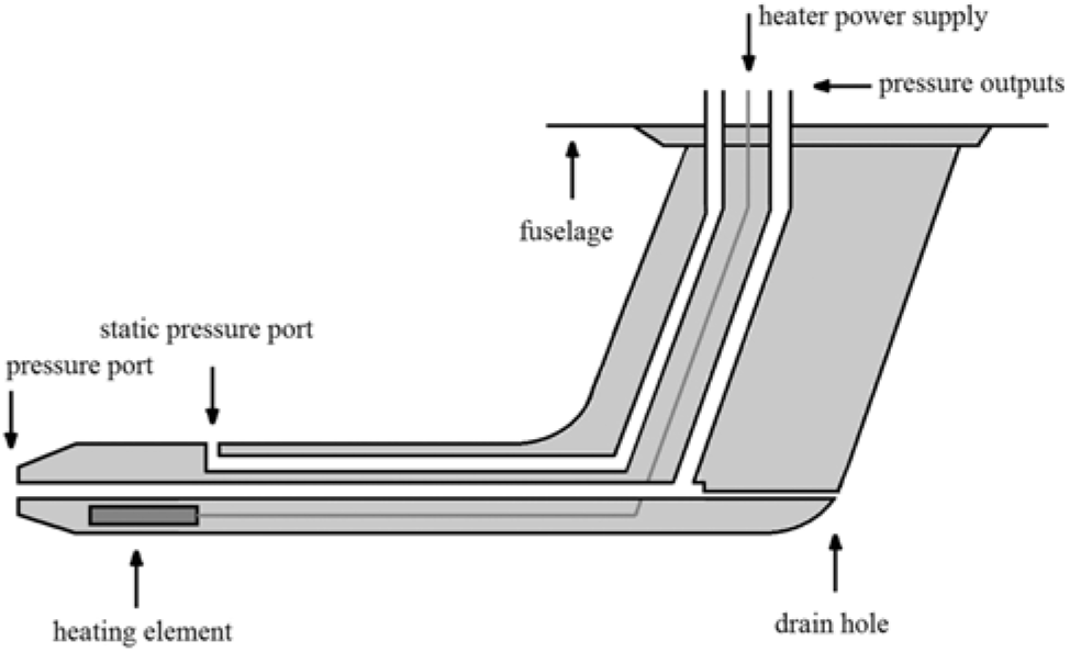
2.0 DESCRIPTION OF THE AERONAUTICAL PITOT PROBE
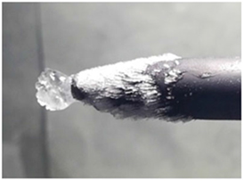
The AN5814 PP, manufactured by Aero Instruments®,is an electrically heated, L-shaped Pitot-static tube, as seen in Fig. 1. It is a very common model, especially for middle and small size aircraft. The schematic diagram in Fig. 1 shows its main components. The stagnation pressure port in the tip measures the total air pressure in order to visualise the aircraft’s speed in the airspeed indicator, while the pressure measurement in the static port is used to determine the aircraft’s altitude, indicated in the altimeter. The electrical heating element shall protect the pressure ports from mechanical obstruction by ice crystals if icing conditions are encountered (Fig. 2).
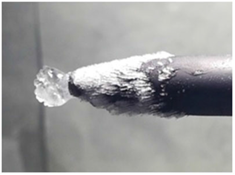
Figure 2. Iced pressure port of the AN5815 Pitot probe.

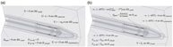
Figure 3. View of the Pitot Probe under study: a) Half sections of the AN5814 Pitot probe; b) Dimensions of the AN5814 Pitot probe (in mm).

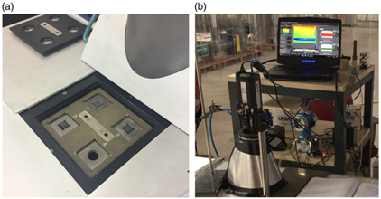
Figure 4. a) Netzsch LFA 447 Nanoflash sample holder with material probes; b) FLIR A655sc IR camera mounted on the test section.
2.1 Inner composition and material properties
In order to obtain more information on its internal structure and material composition, a PP was cut in half along its longitudinal axis. Figure 3(a) shows a close-up view the half section of the PP. It was found that the PP is composed of brassy material (hereinafter referred to as brass) that is coated by a thin layer of a cuprous material (hereinafter referred to as copper). The heat resistant wire is coiled around the leading end of a ceramic-like material acting as an insulator (hereinafter referred to as ceramic). The dimensions, obtained with a Vernier caliper (Mitutoyo Series 530), are presented in Fig. 3(b). Also, the thermal characteristics of the different materials are important for the numerical modelling. In literature, material properties related to these materials are provided. Still, it is difficult to determine their exact material alloy or type. Nevertheless, this information is important due to the fact that, for example in the case of copper, the material properties of its alloys can show significantly different magnitudes among themselves.
Therefore, samples of each material were taken from the PP, as seen in Fig. 3(a). By measuring the weight (precision scale KNWAAGEN KNCD 30/01) and volume (Vernier caliper) of each sample, the mean density of each material was determined indirectly. Using the mean density as the input value, the thermal characteristics of each material could be obtained with a Netzsch LFA 447 Nanoflash. This equipment is able to measure the temperature-dependent specific heat capacity and thermal diffusivity, based on the Flash Method. For this purpose, the material samples, placed in the sample holder Fig. 4(a), are irradiated uniformly from one side, while the surface temperature rise from the opposite site is measured by an IR sensor Fig. 4(b). By correlating the resultant temperature vs time curves with the response of the comparative specimen of materials with known material properties, the temperature-dependent thermal diffusivities of the samples can be determined by an internal regression routine. Simultaneously, as the added irradiation heat Qi, sample mass ms and temperature rise ΔT are known, the specific heat of each sample can be calculated by:
 $$C_p = {{Q_i } \over {m_s \Delta T}}$$
The respective thermal conductivity k can be obtained for each sample using:
 $$C_p = {{Q_i } \over {m_s \Delta T}}$$
3. NUMERICAL CHARACTERISATION: MODELLING OF THE CONJUGATE HEAT TRANSFER
This section presents the modelling of the thermal conditions in a PP caused by heat transfer to the atmosphere in flight conditions in case of a failure of the conventional heating system. The modelling is taken out in CM(15), a multiphysics simulation environment designed to solve partial differential equations over complex geometries based on the Finite Element Method. In order to solve partial differential equations over complex geometries, this method requires the discretisation of the domain into small elements, connected by nodes. Each node is associated with a solution vector. The solution over the element is then inter-polated using a set of shape functions. The element order defines the type of shape function that is used for the inter-polation. For this model, the solution vector of each node contains the fluid velocity, pressure and the temperature. By using a first order element discretisation, all three are inter-polated with linear shape functions. The Backward Differentiation Formula (BDF) scheme, an implicit method to solve initial value problems, was assigned the CM solver to calculate the temporal progress of the phenomena. The solver uses adequate time-stepping algorithms, defined by proposed control tolerances. As a result, larger time steps are taken where the solution changes slowly, while finer time steps are used when the solution gradient in time is strong. The temporal and spatial discretisation were evaluated in a subsequent convergence analysis (Section 5.2.3).
3.1 Physical model assumptions
As demonstrated by Souza(Reference Souza14) in his model, the approximation of a PP with a common geometry as a flat plate surface in parallel flow is valid. The transition from laminar to turbulent flow regime is observed between the Re of approximately 5×10⁵ to 1×10⁶ (16). The critical chord width (Wc) from the PP’s leading edge is then:
 $$W_c = {{Re_c v} \over V}$$
where maximum free stream velocity V is considered to be 85 m s−1, while the kinematic viscosity n at –40°C is 8.614×10⁻⁶ m2 s−1. The resulting critical chord width where the regime transition starts is 0.0501 m. The electrical heating element (EHE) is located in the front part of the PP and takes the dominant role in the conjugate heat transfer (CHT) model. Therefore, CM, and the physic modules of Laminar flow and Heat Transfer in Solids/Fluids were applied on an axis-symmetric domain to model the time-dependent transport phenomena. Both physics were coupled with the non-isothermal flow interface. The flow was treated as compressible; therefore, the fluid density depends on the absolute pressure and temperature. Furthermore, the interface takes into account flow heating due to pressure work and viscous dissipation.
Heat transfer due to radiation between the PP and its surroundings was implemented along the external surfaces. For the solid domains, the material characteristics presented in Section 2 were implemented. Similarly, the Joule heating in the EHE was modelled as a volumetric heat source, based on the power consumption curves obtained.
The model assumptions are viscous Newtonian fluid, external laminar flow regime, subsonic compressible flow and viscosity depending on the temperature. Regarding the solid material properties, these are assumed as temperature-dependent (Section 5). The Joule heating in the EHE is modelled as a volumetric heat source, based on the power consumption curves (Section 5). In addition, radiative heat flow is implemented along the PP’s external surfaces and heat generation is considered due to pressure work.
The solver was chosen as time-dependent and fully coupled. The following paragraphs will describe in more detail the modelling modalities.
3.2 Domain definition
In order to create a model that combines a reasonable computational effort with an acceptable representation of the geometry, a 2D axis-symmetric approximation was chosen. This approach can only be applied from the cylindrical section of the PP. However, since the wing-shaped base is located far from the zone of interest (the pressure ports and heating element), its effect on the corresponding flow and temperature field can be considered negligible. Therefore, it was replaced by an adiabatic wall condition. Figure 5 shows the 2D plane with the corresponding labels for the domains. The domain dimensions are based on Fig 3(b). Domain Ωfluid represents the air flow along the PP. The solids copper, brass and porcelain are part of the solid. Domain ΩHE is composed of circular volumetric heat sources that represent the coils of the heating resistance.
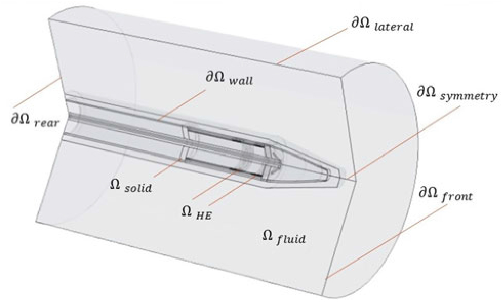
Figure 5. Domain definition of the conjugate heat transfer model.
3.3 Governing equations
In fluid mechanics, the continuity equation is based in the assumption that the fluid properties are continuous functions. Its mathematical formulation is the following:
 $${{\partial \rho } \over {\partial {\rm{t}}}} + \nabla \cdot \left( {\rho u} \right) = 0$$
where ∇ in 2D (r-z), cylindrical coordinates is
 $$\nabla = \vec e_r {\partial \over {\partial {\rm{r}}}} + \vec e_z {\partial \over {\partial {\rm{z}}}}$$
and the velocity vector u in two dimensions has the form
 $${\rm{u}} = \vec e_r u_r + \vec e_z u_z $$
where  $\vec e_r $ and
  $\vec e_z $ are the unit vectors of the velocity components ur and uz, respectively. Because the ∇ operator acts on the vector field u, the dot or scalar product results in a divergence, and Equation 2 eventually yields in
 $$\vec e_z $$
The Navier-Stokes equations are derived from Newton’s second law creating a set of three partial differential equations. Their mathematical formulation is the following:
 $$\vec e_z $$
where the first term corresponds to the inertial, the second represents the relative pressure gradient and the third the viscous forces in the fluid. The fourth term includes all external body forces that act on the fluid (e.g. buoyancy and magnetic forces). Due to the elevated Re of the flow, buoyancy forces acting on the fluid are considered very small. Therefore, the fourth term is neglected in the simulation.
The dynamic viscosity μ is temperature-dependent. Simulating compressible flow implies that the fluid density ρ depends on the absolute pressure and temperature, derived from the ideal gas law:
 $$\rho \left( {{\kern 1pt} p_{abs} ,T_{abs} } \right) = {{p_{abs} M} \over {RT_{abs} }}$$
where M is the molar mass of air 0.02897 kg mol−1, while R is the ideal gas constant with 8.314 J mol−1 K−1. Physically, this means that the fluid’s density variation takes into account both the changes of temperature and the direct dynamics of the pressure field. The required absolute pressure is obtained indirectly based on the relative pressure in the fluid (second term in Equation (6)) and the altitude dependent reference pressure:
 $$p_{abs} = p + p_{ref} $$
The temperature dependence of the fluid properties indicates a coupling with the energy equation:
 $$\rho c_p {{{\kern 1pt} \partial {\rm{T}}} \over {\partial {\rm{t}}}} + \rho c_p u \cdot \nabla T = - \nabla \cdot \left( {k\nabla {\rm{T}}} \right) + Q$$
where term 1 represents the change of thermal energy, while the convective term 2 takes into account the energy transport by fluid motion. Energy transport due to conduction is considered by term 3. Term 4 considers all additional forms of energy added to the domains. At high Re, flow heating by solid–fluid interactions are no longer negligible. Therefore, term 4 considers pressure work Qp and viscous dissipation heating Qvd:
 $$Q = Q_p + Q_{vd} + Q_{gen} $$
where Qgen represents the volumetric joule heating of the EHE, which is located in the solid domain:
 $$Q_{gen} = {{Power\left( t \right)} \over {Volume}}$$
The time-dependent power consumption Power(t) was experimentally obtained (Section 5) for the respective test condition. For the solid domains where heat transfer occurs by conduction only, just terms 1, 3 and 4 need to be solved.
3.4 Initial and boundary conditions
The initial conditions for the thermal and flow transport phenomena are visualised in Fig. 6(a) and 6(b). Initially, velocity is at zero and gets ramped by the inlet condition Vel(t). Solid and fluid temperature are at the same experiment (or flight) temperature, and there is no relative initial pressure. For reproduction of the experiment conditions, Tamb(t) is the data measured by the inlet thermocouple T1 (compare Section 4.1). No slip condition is considered at the wall. Q gen is the Power(t) experimentally obtained in Section 5.1.
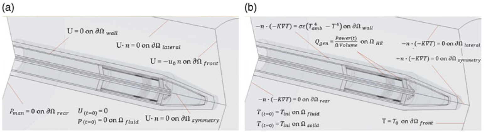
Figure 6. a) Flow initial and boundary conditions of the conjugate heat transfer model; b) Thermal initial and boundary conditions of the conjugate heat transfer model.
3.5 Meshing
The fluid domain Ωfluid, over which the continuity, Navier-Stokes and energy equations will be solved, was divided into three different meshes. Mesh 1 represents the area between the solid domain that is solid up to a perpendicular distance of 10 mm into the fluid (close-field), where the strongest gradients of the solution are expected. Here, a structured mesh, consisting of 3,881 quadrilateral elements was created. The quadrilaterals have a long side length parallel to the solid wall, while the side normal to the wall is relativity short in order to obtain a high element density along the expected solution gradient. Mesh 2, representing the zone from the close-field up to a perpendicular distance of approximately 40 mm into the fluid, was defined as the mid-field. Here, the solution gradient is expected to be weaker and of less directional homogeneity. Therefore, an unstructured mesh of very fine (max. element size 1.6 mm) triangular elements with a small element growth rate (max. 1.03) was created. For the remaining fluid (mesh 3, far-field), where the solution gradients are expected to be very small, a coarse (max. element size 5 mm, max. element growth rate 1.3), unstructured triangular mesh was employed. For solid, over which only the energy equation will be solved, an unstructured mesh of fine (max. element size 2.45 mm) triangular elements with a small element growth rate (max. 1.13) was implemented (mesh 4). A total of 43,522 triangular elements were implemented for the unstructured mesh regions.
4.0 EXPERIMENTAL CHARACTERISATION OF THE AN5815 PITOT PROBE
4.1 Setup and instrumentation
The climatic wind tunnel (CWT) is designed as a closed vertical circuit with a total length of approximately 25.2 m and a test section with the dimensions of 0.3×0.3 m. The air is put in motion by a centrifugal fan, powered by a frequency controlled electric engine. Two evaporator units allow for the controlling of the flow temperature inside the CWT.
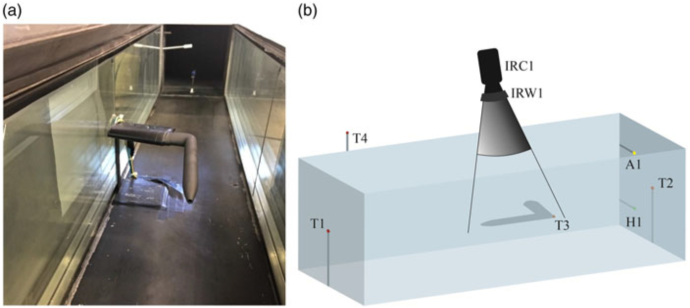
Figure 7. a) Varnished Pitot probe mounted in the centre of the test section, hygrometer and thermocouple T2 are visible in the test section outlet; b) Experiment setup for IR-Thermography with labels of all devices.
Figure 7(a) shows the PP mounted in the test section. Due to their relatively high reflectance, metallic surfaces may reflect background temperatures and are not suitable for reliable IR measurements. Therefore, the PP was varnished with graphite paint (Kontakt Chemie Graphit 33) with an emissivity of 0.97, indicated by the manufacturer. Four thermocouples (TCs) of type K connected to a Data Acquisition Unit (Pico Technology TC-08) were used for real-time temperature measurements during the experiments. They were mounted in the inlet (T1), the outlet (T2) and outside (T4) of the test section to measure the ambient temperature. On the longitudinal end of the PP’s surface (200 mm from the tip), another TC (T3) was attached with thermal grease.
During the experiments, the pressure difference between the PP’s stagnation and static port was measured continuously using a Differential Pressure Transmitter (Endress+Hauser Deltabar S). The pressure difference gives information about free air flow velocity V, derived from the Bernoulli equation, where the flow density ρ is chosen according to the respective free stream temperature inside the CWT during the experiment.
In test section outlet, a hygrometer (H1) for real-time measurements of the relative humidity was installed (DeltaOHM HD 2717T). In Fig. 7, the hygrometer and thermocouple T2 are visible in the test section outlet. The employed IR camera is a FLIR A655sc that measures wavelengths with a microbolometer detector. A scheme of spatial arrangement for the IR Thermography measurements with labels for all devices is presented in Fig. 7(b), where IRC1 and IRW1 are the IR camera and IR inspection window, respectively. A1 represents the dry air inlet required to control the relative air humidity, which was held at approximately 30% for all experiments.
4.2 Experiment design
All runs begin when the CWT, the circulating air and the PP are in quasi-thermal equilibrium. The heating element is switched on to initiate the heating process. Assuring that the PP has reached its quasi-steady-state temperature, the failure of the heating element is simulated. Therefore, after 600 s, the heating element is switched off and the PP’s cooling process is observed for a further 600 s. Both the instantaneous measurements of free stream temperature T and air flow velocity V were time-averaged over the experiment to obtain their mean magnitudes  $$\bar T$$ and
  $$\bar V$$ for each run. The power consumption of the heating element was obtained indirectly by the continuous measurement of tension and current in the PP’s power supply cable.
Table 1 Test conditions for CWT – Experiments

The test conditions 1 to 3 (Table 1) involve three different mean velocities at the respective lowest mean temperature that could be reached in the CWT. The repeatability of the experiments was analysed by comparing the results of test runs under almost the same  $$\bar T$$ and
  $$\bar V$$.
With respect to the measurements taken out in the Netzsch LFA 447, each measuring sequence taken out the respective mean standard deviations σy (indicated in figures in the results) and σx (indicated in table 3) were determined by the flash apparatus. The K-type thermocouples, used for the CWT characterisation, were calibrated in a temperature bath of the type Julabo F25 to obtain their measurement uncertainty σTC.The mean standard deviations for the power consumption σpc and the IR camera measurements σIR were calculated from the results of test conditions 4. By calibration with a water column, the measurement uncertainty of the Differential Pressure Transmitter δDTP was obtained. Furthermore, calibration of the precision scale with monobloc calibration weights was carried out to obtain its measurement uncertainty δPS. Taking further into account the uncertainty of the Vernier caliper δVC, the mean propagation of uncertainty for the density measurements δρ was determined. The specific measurement characteristics of the instruments are presented in Table 3.
5.0 RESULTS AND DISCUSSION

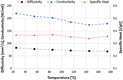
Figure 8. Results of the material analysis for copper as a function of temperature: Thermal diffusivity (σy = 0.59 mm2s−1); conductivity (σy = 1.71 Wm−1∘C−1); specific heat (σy = 0.01 J kg−1∘C−1).
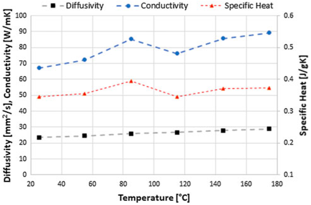
Figure 9. Results of the material analysis for brass as a function of temperature: Thermal diffusivity (σy = 0.38 mm2s−1); conductivity (σy = 0.22 Wm−1∘C−1); specific heat (σy = 0.01 J kg−1∘C−1).
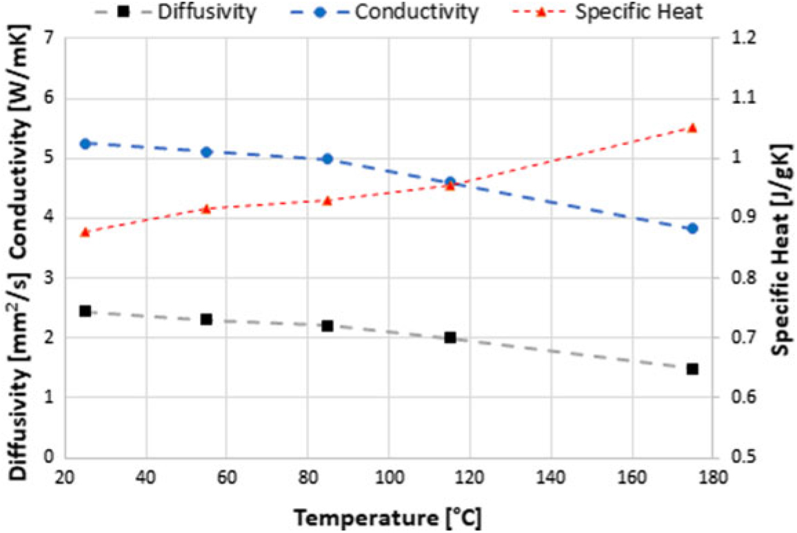
Figure 10. Results of the material analysis for ceramic: Thermal diffusivity (σy = 0.05 mm2s−1); conductivity (σy = 1.12 Wm−1∘C−1); specific heat (σy = 0.04 J kg −1∘C−1).
5.1 Material characterisation
Density values for cooper, brass and ceramic were 7,236 kg/m3, 8,335 kg/m3 and 2,401 kg/m3 respectively.
Figures 8 to 10 show the results obtained for the material characterisation with the Flash Method. Two samples of the same material were placed in the sample holder of the Netzsch LFA 447 Nanoflash and analysed simultaneously.
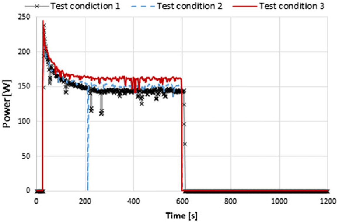
Figure 11. Power consumption of the heating element vs time for test conditions taken out in the CWT: test condition 1, 2 and 3.
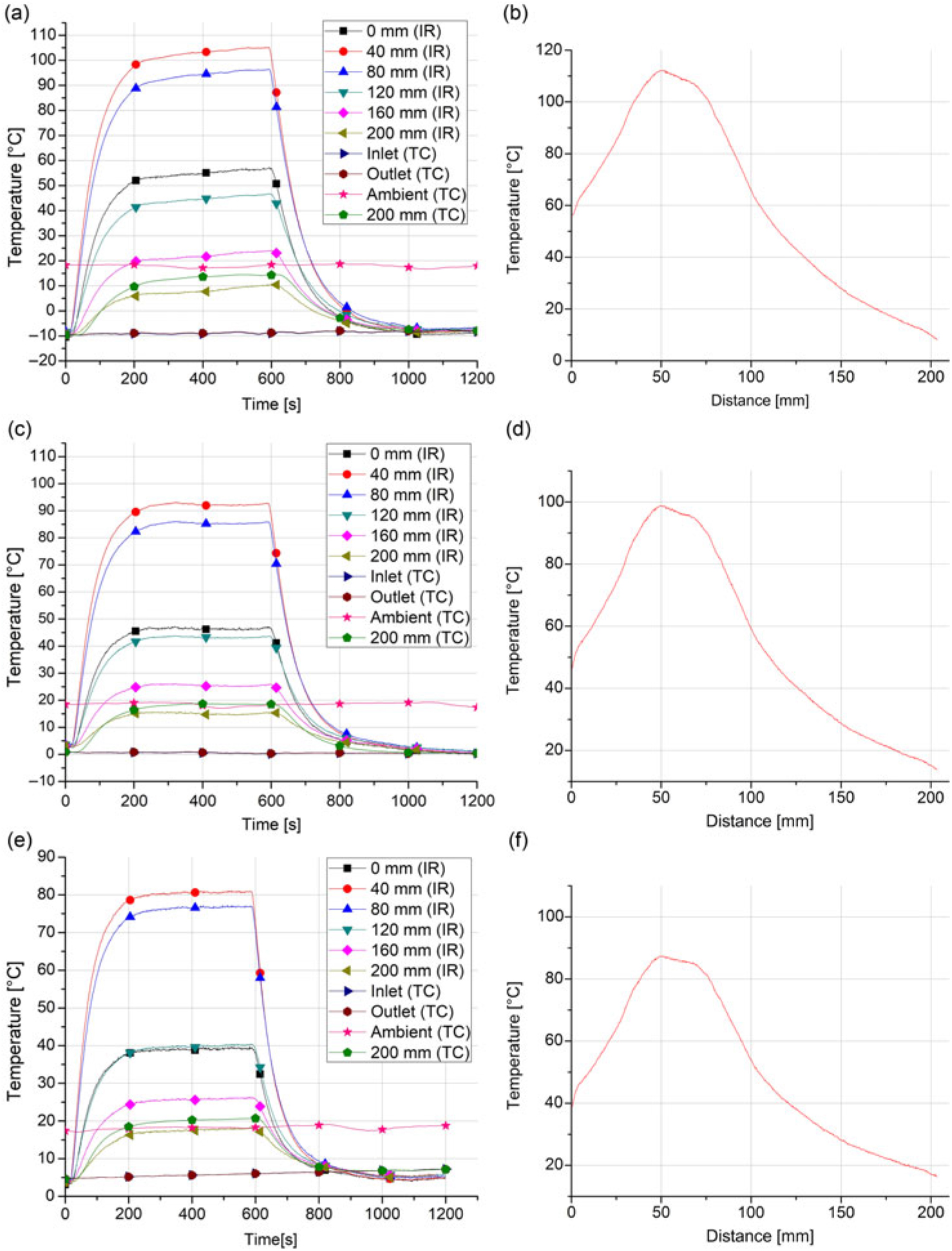
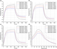
Figure 12. Results of CWT test runs: Local transient temperatures and steady-state temperatures along the PP.
Due to the power consumption curves (Fig. 11), it is assumed that the heater resistance is temperature-dependent. Directly after switch-on, the power consumption is at the maximum, followed by an exponential decay and eventually stabilising at a steady-state magnitude. In addition, this magnitude depends on the operating conditions, being higher for larger heat extraction (caused by higher flow velocities).
Figures 12(a), 12(c) and 12(e) show the results for the transient local temperatures measured on the PP’s surface as well as inside and outside the test section measured with the IR camera and the thermocouples. Here, the temperature behaviour of the tip is of a particular interest due to the tendency of ice accretion on its leading edges, which eventually leads to the clogging of the stagnation pressure port.
The time period until the tip cools down to the free stream temperature is approximately 960, 1,090 and 830 s for the test conditions 1, 2 and 3, respectively. The longitudinal steady-state temperatures along the PP are presented in Figs. 12(b), 12(d) and 12(f) for the respective test conditions 1, 2 and 3. For each test condition, the maximum temperatures occur in the section where the heating element is installed. The respective thermal response and power consumption in the repeatability analysis were very similar. The mean standard deviation for the power consumption was 1.39 W, while for the thermal performance measurements the mean standard deviation was 0.95∘C and 0.23∘C for the transient tip temperature and the longitudinal steady-state temperature, respectively.

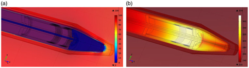
Figure 13. a) A solution of the flow field around the Pitot probe; b) A solution of the temperature field on the Pitot probe.
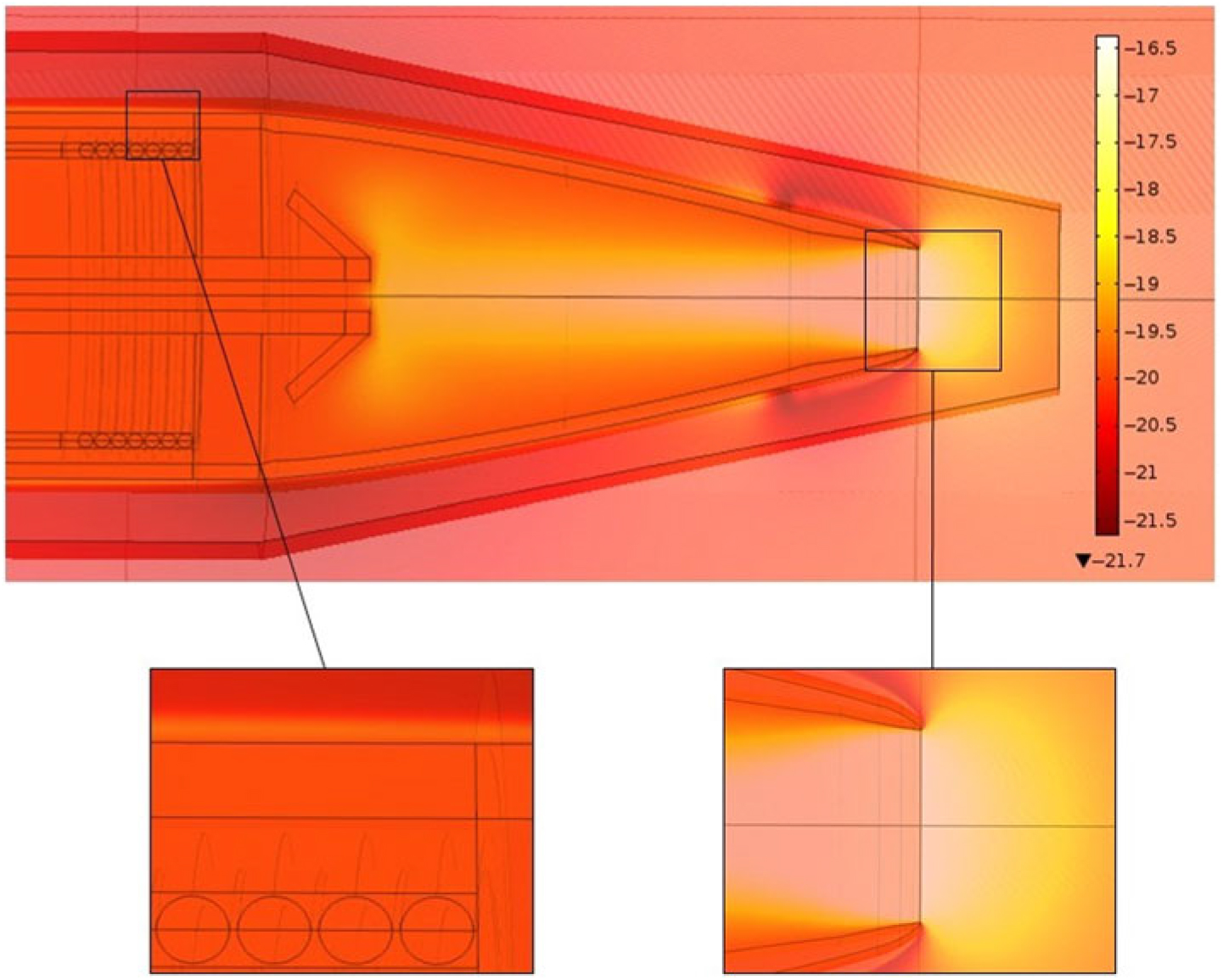
Figure 14. Viscous and pressure heating effects at an ambient temperature of −20∘C and an airspeed of 85 ms−1.
Table 2 Measurement instrument characteristics

5.2 Validation of the model
5.2.1 Qualitative analysis of the numerical results
Figures 13(a) and 13(b) illustrate arbitrary solutions of the flow and temperature fields on and around the PP with EHE in operation. For all solutions of the flow and temperature field, the colour bars correspond to the units of ms−1 and degrees Celsius, respectively. As expected, the strongest solution gradients in both the flow and temperature field are located in the boundary layer. Furthermore, in Fig. 13(a), the stagnation point is easy to identify in front of the PP’s tip.
Figure 14 shows the temperature field solution with switched-off heating elements at an ambient temperature of −20∘C and an airspeed of 85 ms−1. Here, the importance of the viscous and pressure heating effects can be observed in the boundary layer and the stagnation point, respectively.
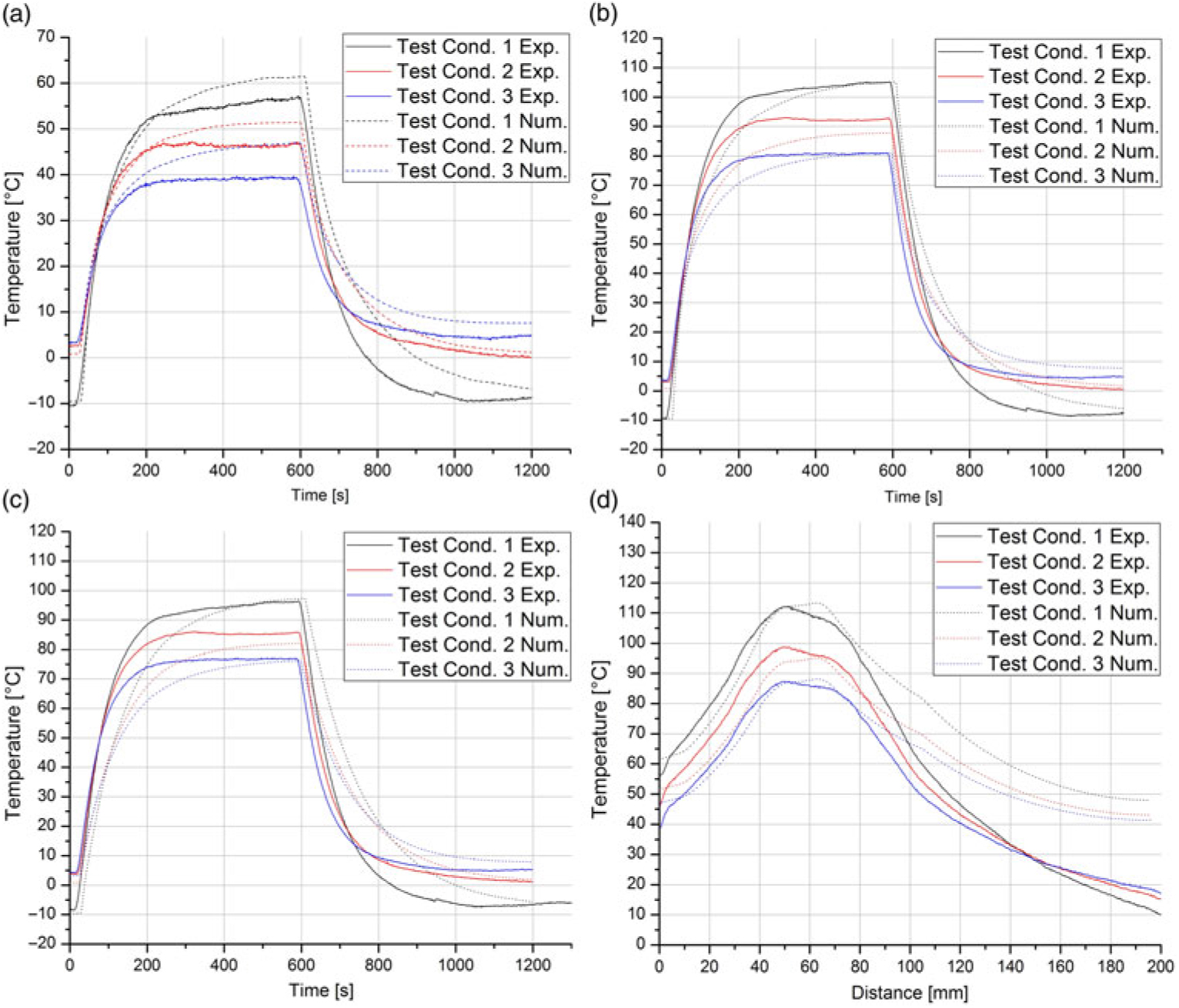
Figure 15. a) Comparison between experimental and numerical results for tip temperature behaviour during intermittent heating element operation; b) 40 mm from tip; c 80 mm from tip; d longitudinal steady state temperature along Pitot probe.
5.2.2 Comparative analysis between experimental and numerical results
In order to evaluate the validity of the model, the following figures show the thermal behaviour of the PP’s surface together with the corresponding data of the test runs (test conditions 1, 2 and 3 of Table 2) taken out in the CWT. Furthermore, the overall local relative error for each local temperature measurement and the power consumption was calculated. The calculation of the relative error is based on the average value of the experimental and numerical results. Figures 15(a), 15(b) and 15(c) show the comparisons of the temperature behaviour during intermittent heating element operation at the tip, 40 mm and 80 mm from the tip, respectively.
The mean relative error for the tip temperature simulation results in 17.41%, while the temperature measurement of 40 mm from the tip has a magnitude of 13.22%. Figure 15(d) shows the comparison between the experimental and numerical results of the longitudinal steady-state temperature along the PP for the conditions of the three test runs taken out in the CWT.
The mean relative error for the temperature measurement of 80 mm from the tip results in 19.36%, while for the longitudinal steady-state temperature, it has a magnitude of 20.53%. For all transient temperature curves, it can be seen that, in general, the model has more thermal inertia compared to its real counterpart, which reaches its steady state earlier and cools down faster. The simulation of test condition 1 for all measurements leads to the least accurate results for this case. Regarding the steady state temperatures, Fig. 15(d) shows that the results are acceptable up to a distance of 80 mm from the tip. After 80 mm, the predicted temperature of the model is remarkably higher than obtained in the experiment. In the view of the authors, this discrepancy is the result of the certain modelling simplifications. First, as it can be seen in Fig. 15(d), the experimental temperatures show a gradient at 200 mm, while for the model in this location an insulating boundary was implemented. Furthermore, due to the model’s axis-symmetric approach, the rear geometry of the PP was simplified. In addition, in Section 3.1 the resulting critical chord width, where the flow begins to get turbulent, was calculated as 0.0501 m. As the flow was modelled laminar along the whole PP, this could introduce an additional factor related to the difference between experimental and numerical results. Similar problems were encountered in the model presented by Souza(Reference Souza14). Nevertheless, as the rear section of the PP was considered as the least important part of the simulation (compare with Section 3.1), the model is considered suitable to simulate the thermal response in flight conditions.
5.2.3 Convergence analysis
The convergence analysis was taken out for the flight conditions (Section 5.3), being aware that here the boundary conditions and, therefore, the solution gradients are the strongest, which makes the results more sensible to convergence errors due to poor temporal and spatial discretisation.
Therefore, the mesh density was increased step-by-step in order to evaluate when the relative variance of the solution becomes negligible. First, it is important to reasonably define a solution parameter and in which location its evaluation will be taken out. In a CHT problem, the thermal solid–fluid interaction is strongly dependant on the velocity gradient of the aerodynamic boundary layer. Therefore, the element density of the corresponding mesh 1 (Section 3.5) was altered in order to evaluate the effect on the solution of the U component along the boundary layer. Figure 16 shows the U component solution for the different numbers of quadrilateral elements in the aerodynamic boundary layer.
Also, the dependence of the steady-state temperature along the PP to the number of quadrilateral elements in the thermal boundary layer was evaluated. Figure 16(b) shows the solution of the longitudinal steady-state temperature for the different numbers of quadrilateral elements in the thermal boundary layer.
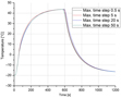
Regarding the temporal discretisation, for an explicit event in time (here the time dependent load of the EHE), caution is advised. Here, if the time stepping is too loose, the solver may inter-polate over relevant parts of the event, assuming a non-existing linearity of the solution. Therefore, the dependence of the solution on the temporal discretisation of the phenomenon was analysed. Figure 17 shows the transient tip temperature for different permitted time steps taken by the solver.
The convergence analysis has shown that an increase from 10 to 15 boundary layer elements results in no further relevant variation of the solution. Likewise, it was ensured that the temporal discretisation of the phenomenon was adequate to obtain an acceptable solution accuracy and, furthermore, capture the time-dependent loads. Amongst all simulations, the operation of the in-flight condition resulted in the strongest solution gradients, and the present analysis is further suitable to ensure the convergence of the foregoing simulations with input conditions of the test runs taken out in the CWT.
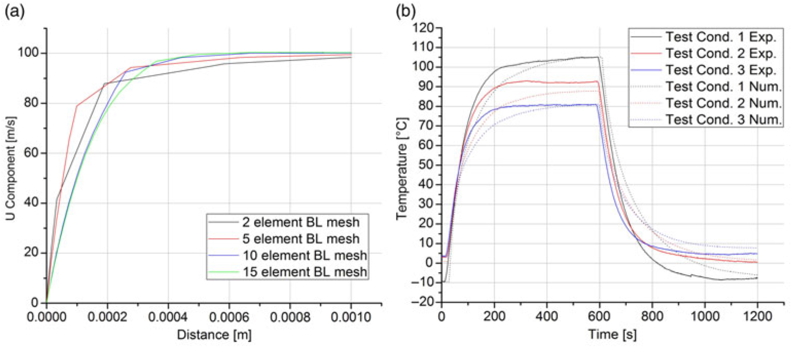
Figure 16. Convergence analysis for different numbers of quadrilateral elements in the aerodynamic boundary layer (BL): a) the steady state U component; b) longitudinal steady state temperature along the Pitot probe.
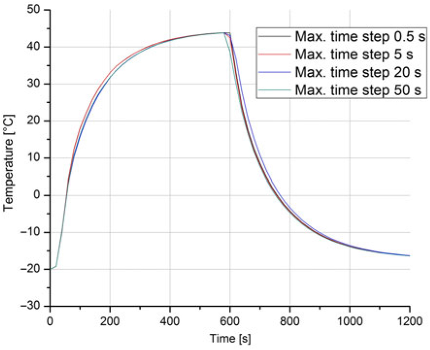
Figure 17. Convergence analysis of the transient tip temperature for different maximum time steps taken by the solver.
5.3 Simulation of operation in flight conditions
After the CHT model has been validated in the foregoing, the objective of this section is to provide the model with input data that represent the operation of the PP in flight conditions. In order to demonstrate one possible application of this model, the failure of the conventional heating system is simulated in order to obtain the time until the PP reaches a temperature where ice formation can be expected (e.g. due to a malfunction of the heating system). As a reference, the typical operating conditions encountered by an Embraer EMB 110 were chosen. This twin-turboprop aircraft is mainly employed as a regional airliner. Based on a cruise speed of 85 ms−1 and an operating altitude of 18,000 ft over sea level, the corresponding ambient air conditions were obtained according to the International Standard Atmosphere (ISO 2533). Furthermore, the time-dependent power consumption curve of test condition 3 was implemented as input data. The following figures show the solutions for the thermal response of the PP’s surface during flight conditions. Figure 18(a) illustrates the temperature behaviour during intermittent heating element operation at the tip, 40 mm, 80 mm and 120 mm from the tip, respectively. In Fig. 18(b), the longitudinal steady-state temperature along the PP is presented.
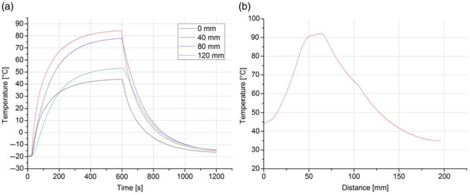
Figure 18. a) Flight conditions – Temperature behaviour during intermittent heating element operation; b) Flight conditions – Longitudinal steady state temperature along Pitot probe.

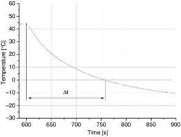
Figure 19. Flight conditions – Tip temperature response after heating element failure.
In Fig. 19, a magnified view of the tip temperature response after a heating element failure at 600 s is presented. The time interval Δt = 165 s after the EHE is switched off; the tip temperature undercuts the zero degrees Celsius mark. As observed in Jäckel et. al.(Reference Jäckel and Gutiérrez Urueta17), surface icing on the PP’s tip can occur from this moment onwards. This is a necessary, but insufficient condition, for in-flight icing. There are other factors, e.g. the liquid water content in the air (LWC) and the droplet size, which determine if and how ice formation occurs. Nevertheless, the idea of this exercise is to give an estimation of how much time the pilots would have left to react to a heating element failure before icing could theoretically occur due to the low PPP’s tip surface temperature under least favourable ambient conditions. For this reason, the phenomena of ice formation itself is not considered in the physics modelling. In the case of a failure of the heating system, usually the pilot receives a fault signal that can be from the heating switch LED or, in commercial aircraft, through the board computer display. Especially for smaller and mid-size aircraft with only one PP, a heating failure requires immediate response. Particularly, the pilot is required to manoeuvre the aircraft towards meteorological conditions in which Pitot icing is least probable(Reference Landsberg1). This is likely possible due to the fact that icing clouds are strongly limited in their vertical extension. Studies have pointed out that 90% of the clouds with icing risk have a vertical dimension of less than 3,000 ft(3). Still, the ability to safely leave an icing cloud, when facing a PP heating malfunction, depends basically on the time in which the PP remains protected against icing. This conclusion is also reinforced by the fact that even a short time with erroneous PP readings can result in fatal reactions of the pilot. A prime example is the Air France 447 incident where the incorrect readings on the primary flight display were erroneous for only 29 s(18). This relatively short period of time induced sufficient confusion in the cockpit to cause the tragic outcome.
6.0 CONCLUSIONS
In this research, a numerical model to simulate the thermal behaviour of an AN5814 PP was created using CM. By implementing test conditions as input data for the simulations and comparing the experimental results with their numerical counterparts, it was possible to validate the model. After the CHT model had been validated, the model was fed with input data that represent the operation of the PP during flight conditions typically encountered by an Embraer EMB 110. The failure of the conventional heating system was simulated in order to obtain the time until the PP reaches a tip temperature where ice formation can be expected. The tip temperature undercut the zero degrees Celsius mark 165 s after the EHE was switched off. Eventually, a convergence analysis was taken out to ensure that the variation of the solution after the refinement of the domain and temporal discretisation stays negligibly small.
A variety of experiments was conducted in order to characterise a commercial aeronautic PP. First, the inner composition and dimensions of the PP were presented. It was found that the PP is mainly composed of cuprous, brassy and ceramic materials. The thermo-physical characteristics of these main materials were analysed using the Flash Method:
• The thermal conductivity, diffusivity and specific heat for each material were obtained.
Performance runs in the CWT allows visualising the following:
• The power consumption shows a maximum after switch-on and eventually stabilises at a steady-state magnitude, being higher for larger heat extraction.
• The time interval until the tip cools down to the free stream temperature was determined for the test conditions presented.
The data collected in this work can be used to implement and validate mathematical models in order to predict the thermal performance of Pitot probes in flight conditions.
ACKNOWLEDGEMENTS
The Mexican Council for Science and Technology (CONACyT) funded this work and was supported by the Faculty of Engineering of Autonomous University of San Luis Potosí (UASLP) and Interdisciplinary Centre of Fluid Dynamics (NIDF), which is part of the Federal University of Rio de Janeiro.