2.1. Problem formulation and model description

We consider a two-dimensional permeable cylindrical shell of diameter $D$ subject to an incompressible flow of a Newtonian fluid of constant density $\rho$ and viscosity $\mu$, whose free-stream velocity is $U$, as depicted in figure 1. The cylindrical shell is constituted of a monodisperse repetition of solid inclusions, whose characteristic length scale is denoted as $\ell$. Since $\ell \ll D$ we can introduce a separation-of-scales parameter defined as the ratio between the two length scales at play:

(2.1)\begin{equation} \varepsilon:=\frac{\ell}{D} \ll 1. \end{equation}

Under this assumption, a homogenized model is employed to describe the flow through the membrane (Zampogna & Gallaire Reference Zampogna and Gallaire2020), which is macroscopically represented by a smooth surface with zero thickness. In the outer and inner pure-fluid regions split by the permeable shell, the incompressible Navier–Stokes equations hold. The velocity $\boldsymbol {u}^*$ and pressure $p^*$ fields are introduced, where the superscript $^*$ denotes dimensional variables. Introducing the Cartesian coordinate system $(x_1,x_2)$ (figure 2), these equations read ($i,j=1,2$)

(2.2)\begin{equation} \left. \begin{gathered} \rho {\partial}^*_{t} {u}^*_{i}+\rho {u}^*_{j} {\partial}^*_{j} {u}^*_{i} ={-}{\partial}^*_{i} {p}^*+\mu {\partial}^{*2}_{jj} {u}^*_{i},\\ {\partial}^*_{i} {u}^*_{i} =0. \end{gathered} \right\} \end{equation}

The flow through the membrane is described by an effective stress jump model, consisting of the discontinuity in the fluid stress and the continuity of velocity across the permeable shell, denoted here with $\varGamma _{{int}}$ (red line in figure 1). Labelling with the superscript $^-$ and $^+$ variables evaluated respectively in the outer and inner fluid regions, as shown in figure 1, the interface conditions at the membrane $\varGamma _{{int}}$ read ($i,j,k=1,2$)

(2.3)\begin{equation} \left. \begin{gathered} {u}^*_{i}={u}^{*+}_{i}={u}^{*-}_{i}, \\ {u}^*_{i}=\frac{\ell}{\mu}{\mathsf{M}}_{i j} \left( {\varSigma}^{*}_{j k}\left(p^{*-},\boldsymbol{u}^{*-}\right) -{\varSigma}^{*}_{j k}\left(p^{*+},\boldsymbol{u}^{*+}\right) \right)n_k, \end{gathered} \right\} \end{equation}

where ${\varSigma }^{*}_{j k}$ is the $jk$th component of the stress tensor defined as

(2.4)\begin{equation} {\varSigma}^{*}_{j k}\left(p^*,\boldsymbol{u}^*\right) ={-} p^{*}\delta_{jk}+\mu(\partial^*_j u_k^{*}+\partial^*_k u_j^{*}), \end{equation}

and the components of the tensor ${\mathsf{M}}_{i j}$ (figure 1) are

(2.5)\begin{equation} {\mathsf{M}}_{i j}=\bar{L}_t t_i t_j -\bar{F}_n {n}_i {n}_j, \end{equation}

where $\bar {L}_t,\,\bar {F}_n$ are evaluated by solving microscopic problems within the elementary unit cell introduced in figure 1, in the local reference frame $(\boldsymbol {t},\boldsymbol {n})=((-\sin (\alpha ),\cos (\alpha )), (\cos (\alpha ),\sin (\alpha )))$ (see Zampogna & Gallaire (Reference Zampogna and Gallaire2020) and § 4.2 for a detailed description of these problems and their solution). We note that the generic tensor ${\mathsf{N}}_{ij}$ of the original condition developed in Zampogna & Gallaire (Reference Zampogna and Gallaire2020) is replaced here by $-{\mathsf{M}}_{ij}$ since, in the present work, we consider only solid inclusions which are symmetric with respect to $\varGamma _{int}$ and we assume that inertia is negligible within the pores.

Figure 1. (a) Fluid flow configuration considered in the present work and its typical structure past the cylindrical permeable shell ($\varGamma _{{int}}$, in red) of diameter $D$, where we denote the length of the recirculation region $L_R$ and its distance $X_R$ from the rear of the body. The angle $\alpha$ is measured counterclockwise starting from the rear. The superscript minus sign indicates that the generic variable $f$ is evaluated in the outer fluid region while the superscript plus sign refers to the inner fluid region. (b) Zoom on the shell to highlight its microscopic structure in cylindrical coordinates, made by replication of solid inclusions denoted by $\mathbb {M}$ with boundary $\partial \mathbb {M}$ and sketch of the elementary unit cell in dashed line, whose tangential-to-surface size is $\ell$. The fluid domain within the unit cell is denoted by $\mathbb {F}$ while its upper and lower boundaries are indicated, respectively, with $\mathbb {U}$ and $\mathbb {D}$.

Figure 2. Computational domain considered in the present work. The regions denoted with $N_j$ represent the different mesh refinements used when approaching the permeable shell. At the inlet $\varGamma _{{in}}$ a free-stream condition with a Dirichlet boundary condition of the form $u^*_1=U$ and $u^*_2=0$ is imposed, while on the lateral boundaries $\varGamma _{{lat}}$ and at the oulet $\varGamma _{{out}}$ the stress-free condition $(-p^*\delta _{ij}+\mu \partial ^*_j u^*_i)n_j=0$ is used. On the interface $\varGamma _{{int}}$ conditions (2.3) are imposed.

By considering $D$ and $U$ respectively as reference length and velocity scales, we obtain the following system of non-dimensional equations:

(2.6)\begin{equation} \left. \begin{gathered} {\partial}_{t} {u}_{i}+ {u}_{j} {\partial}_{j} {u}_{i} ={-}{\partial}_{i} {p}+\frac{1}{Re} {\partial}^{2}_{jj} {u}_{i},\\ {\partial}_{i} {u}_{i} =0, \end{gathered} \right\} \end{equation}

where we introduce the Reynolds number as $Re={\rho U D}/{\mu }$. The non-dimensional interface condition on $\varGamma _{{int}}$ reads

(2.7)\begin{gather} \left. \begin{gathered} {u}_{i}={u}^{+}_{i}={u}^{-}_{i}, \\ {u}_{i}=Re\mathcal{M}_{i j} \left(\varSigma_{jk}\left(p^-, \boldsymbol{u}^-\right)-\varSigma_{jk}\left(p^+, \boldsymbol{u}^+\right) \right)n_k , \end{gathered} \right\} \end{gather}

(2.8)\begin{gather} {\varSigma}_{j k}(p,\boldsymbol{u})={-} p\delta_{jk}+\frac{1}{Re}(\partial_j u_k+\partial_k u_j), \end{gather}

(2.9)\begin{gather} \mathcal{M}_{i j}=\mathcal{L} t_i t_j -\mathcal{F} {n}_i {n}_j , \end{gather}

where $\mathcal {L}=\epsilon \bar {L}_t$ and $\mathcal {F}=\epsilon \bar {F}_n$ are respectively labelled as slip and filtrability numbers. The interface condition (2.7) thus states that the velocity at the membrane is proportional to the Reynolds number and to the tensor $\mathcal {M}_{ij}$. According to Zampogna & Gallaire (Reference Zampogna and Gallaire2020), the tensor $\mathcal {M}_{ij}$ describes the geometry of the microscopic problem with negligible inertial effects within the microscopic domain, in a non-dimensionalization which makes the problem independent of the macroscopic Reynolds number. In the macroscopic perspective, the relative importance between inertial and viscous effects is taken into account by $Re$ in (2.7). More specifically, the velocity locally tangential to the interface is proportional to $\mathcal {L}$, while the normal velocity is proportional to $\mathcal {F}$. Therefore, the filtrability and slip numbers denote the capability of the flow to pass through and slip along the membrane, respectively. Different limiting behaviours of the interface condition (2.7) are thus identified. When $\mathcal {F}=0$, the flow cannot pass through the membrane but it can slip along it. This situation is analogous to the one outlined in Zampogna, Magnaudet & Bottaro (Reference Zampogna, Magnaudet and Bottaro2019) for rough surfaces, and the resulting boundary condition is formally analogous to the so-called Navier slip condition. When $\mathcal {L}=0$, a no-slip condition is imposed on the tangential velocity, while the normal one varies in proportion to $\mathcal {F}$. This situation can be interpreted as an averaged Darcy law through the membrane, where the viscous effects and thus the slip at the interface are neglected (Zampogna & Bottaro Reference Zampogna and Bottaro2016). Other limiting cases occur for $\mathcal {F}=0$ and $\mathcal {L}=0$, which corresponds to a solid wall condition, and for $\mathcal {F} \rightarrow \infty$ and $\mathcal {L} \rightarrow \infty$, which corresponds to the imposition of the continuity of stresses across the microscopic elementary volume whose size tends to zero, and thus to the absence of the solid structure. Since the flow configuration is solved numerically, we refer to the caption of figure 2 for an explanation of the boundary conditions imposed on the remaining boundaries of the computational domain. These conditions, in non-dimensional form, read $u_1=1$, $u_2=0$ at the inlet and $(-p\delta _{ij}+({1}/{Re})\partial _j u_i)n_j=0$ on the lateral and outlet boundaries.

2.2. Homogenization-based design

In the existing literature, works on permeable bodies and membranes were focused on the evaluation of the macroscopic parameters of the membrane (slip and filtrability) starting from the microscopic geometry. Other works treated the above-mentioned macroscopic quantities as free parameters in order to characterize, modify and optimize the fluid flow surrounding the porous body, without providing an explicit link between these parameters and the microscopic structure of the membrane. Here, we propose to fill the gap between these two aspects by an inverse formulation of the homogenized model that, on the one hand, is extremely efficient for parametric studies and, on the other hand, allows one to deduce the microscopic geometry which realizes given distributions of $\mathcal {L}$ and $\mathcal {F}$.

The inverse formulation aims at deriving the microscopic characteristics of the membrane based on the macroscopic features of the steady flow. In the present paper, an efficient workflow for deducing full-scale structures starting from the homogenized model is adopted (cf. the top frame of figure 3). The generic workflow therefore firstly consists of an analysis where the homogenized model is employed. The implementation of the homogenized model implies a decoupling between the microscopic structure and the macroscopic effect on the flow. On the one hand, parametric studies and optimizations are simplified owing to the reduced number of parameters; on the other hand, the retrieval of the full-scale structure is performed in a second step, when the macroscopic feedback embodied in the scalar parameters of the homogenized model is already known.

Figure 3. (a) Generic workflow to efficiently analyse a flow configuration via homogenized models integrated in classical analyses like, for instance, parametric studies, stability analysis or adjoint-optimization finalized to identify configurations of interest. The retrieval of the full-scale physics for the identified configurations is done in a last step leading to a substantial reduction of the complexity of the optimization problem. (b,c) The generic workflow has been specialized in the present paper for the design of permeable membranes. Colours and red numbers are used to correctly place each step of the procedure adopted in the present paper in the generic workflow. A homogenized model is used to characterize a specific flow configuration in a direct formulation. This allows one to identify a set of objectives and the corresponding values of the macroscopic parameters realizing these objectives. Homogenization is then used in an inverse formulation to associate the values of the macroscopic tensors with a specific microscopic geometry.

For illustration purposes, the workflow is specialized to analyse the flow configuration shown in figure 1, leading to the following procedure:

1. (i) Using the homogenized approach described in the previous section, we perform a parametric study for varying $\mathcal {L}$ and $\mathcal {F}$, by solving the steady version of (2.6)–(2.7) for different values of the Reynolds number.

2. (ii) We characterize the topological properties of the steady flow (e.g. the characteristic dimensions of the recirculation region) and the aerodynamic/hydrodynamic properties of the permeable shell, such as its drag coefficient.

3. (iii) The validity of the performed investigation, carried out assuming that the flow is steady, is verified by linear stability analysis (Chomaz Reference Chomaz2005; Theofilis Reference Theofilis2011). The latter has the advantage of characterizing the stability of the steady solution with a computational cost comparable with that needed to compute steady solutions, thus making it suitable for the performed parametric study.

4. (iv) Once the variety of possible steady solutions is reduced by excluding the unstable configurations, for which the steady analysis would be inappropriate, the objective to be optimized is defined, e.g. the maximum drag coefficient for a fixed Reynolds number. Therefore, the values of $\mathcal {L}$ and $\mathcal {F}$ that maximize the objective function are identified. This can be done by employing adjoint procedures for spatially homogeneous membrane properties. However, since in this work we perform a parametric study, the values are directly deduced from the latter.

5. (v) We then move from the macroscopic perspective to the microscopic one, aiming at identifying the geometry of the membrane that corresponds in macroscopic terms to the optimal configuration previously identified. We therefore perform the microscopic simulations described in Zampogna & Gallaire (Reference Zampogna and Gallaire2020) for a fixed geometry by varying the fluid-to-solid ratio of the porous shell. We thus define the microscopic geometrical parameters and $\varepsilon$.

6. (vi) We eventually verify the accuracy of the resulting structure by comparing the full-scale simulations with the homogenized results.

The outlined technique has the great advantage of markedly reducing the complexity of the problem and giving a parametric map of the properties of the flow by varying the microscopic geometry of the membrane. An extension of this technique to treat the case of a microscopic geometry that varies along the membrane is obtained by a gradient-based optimization implemented via a Lagrangian approach, detailed in § 5.2. In particular, we consider as a starting point the configuration, with constant slip and filtrability numbers, that maximizes the drag coefficient. We evaluate the sensitivity of this predefined objective function (drag maximization) with respect to spatial inhomogeneities of the properties of the membrane and perform a gradient-based optimization. The resulting structure is then obtained by following an inverse procedure based on the microscopic calculations of Zampogna & Gallaire (Reference Zampogna and Gallaire2020), but extended to the case of variable properties along the membrane.

We finally underline that the procedure, illustrated here for the specific case of a wake flow, is of general validity and can thus be applied to a generic flow.

3.1. Steady flow characterization

The steady wake past a circular solid cylinder is characterized by a recirculation region that is symmetric with respect to the $x_1$ axis. We denote with $(\boldsymbol {U},P)$ the steady solution of (2.6). Since, by construction, we do not introduce any further asymmetry, also the flow past the permeable cylindrical shell is expected to be $x_1$-symmetric. For this reason, we only report the flow field in the region $x_2>0$. For the present analysis, we introduce the length of the recirculation region $L_R$ and its distance from the rear of the body $X_R$ as defined in figure 1. In figure 4 we report the flow streamlines for different values of $\mathcal {F}$ when $Re=50$ and $\mathcal {L}=10^{-4}$. At low values of $\mathcal {F}$, e.g. $\mathcal {F}=10^{-4}$, the wake is similar to the solid case, i.e. characterized by a recirculation region attached to the rear of the cylinder ($X_R\approx 0$). As the value of $\mathcal {F}$ increases, the recirculation region detaches from the body and moves downstream. A further increase in $\mathcal {F}$ implies a size reduction of the recirculation region ($L_R$), and at very large values of $\mathcal {F}$, i.e. $\mathcal {F}=3 \times 10^{-2}$, the recirculation region eventually disappears ($L_R=0$).

Figure 4. Streamlines of the flow past the cylindrical permeable shell at $Re=50$ for $\mathcal {L}=10^{-4}$ and four different values of $\mathcal {F}$: (a) $\mathcal {F}=10^{-4}$, (b) $\mathcal {F}=10^{-3}$, (c) $\mathcal {F}=10^{-2}$ and (d) $\mathcal {F}=3 \times 10^{-2}$.

In figure 5 we report the variation of the recirculation region with $\mathcal {F}$, for different slip numbers $\mathcal {L}$ and for $Re=50$. Independently of the value of the slip number, a behaviour similar to that described in figure 4 is observed. For a fixed filtrability number, an increase in $\mathcal {L}$ leads to a slight decrease of $L_R$, while $X_R$ does not vary noticeably.

Figure 5. (a–d) Streamlines identifying the recirculation region past the cylindrical permeable shell at $Re=50$ for different values of $\mathcal {F}$. Each panel corresponds to a single value of $\mathcal {L}$.

A complete characterization of the flow morphology requires also the analysis of the effect of the Reynolds number. In figure 6 we show the recirculation regions for fixed filtrability number $\mathcal {F}= 10^{-2}$, for different values of $\mathcal {L}$ and for $Re=50$, 75, 100 and 110. For $Re=50$, the flow is characterized by a recirculation detached from the body such that $L_R\approx 2$. At $Re=75$, the recirculation region moves downstream and $L_R$ increases. This effect is enhanced at large values of the slip number. In the last case, $Re=110$, the recirculation region moves further downstream and $L_R$ decreases, and eventually disappears for large values of $\mathcal {L}$.

Figure 6. (a–d) Streamlines identifying the recirculation region past the cylindrical permeable shell at $\mathcal {F}=10^{-2}$ and for different values of $Re$ and $\mathcal {L}$. Note that for $\mathcal {L}=3\times 10^{-2}$ and $Re=110$, recirculation is suppressed.

The evolution of $L_R$ and $X_R$ with $\mathcal {L}, \mathcal {F}$ and $Re$ is summarized in figure 7. The quantities $L_R$ and $X_R$ have been deduced by a Matlab script which evaluates the position of the zeros of the horizontal velocity field sampled on the line $x_2=0$. In analogy with the solid case, $L_R$ increases with $Re$ (figure 7$a$). The curves are grouped in clusters. Each cluster represents different values of $Re$, and each curve within the cluster a different value of $\mathcal {L}$. For $Re=25$, $L_R$ decreases with $\mathcal {F}$ until the recirculation region disappears for $\mathcal {F} \approx 10^{-2}$. A similar trend is observed for $Re=50$, but in this case the recirculation region disappears for larger values of $\mathcal {F}$. For $Re>50$, interestingly, the recirculation region grows as the filtrability number increases. The value of $L_R$ reaches a maximum and decreases, until the recirculation region disappears for $\mathcal {F} \approx 1.5 \times 10^{-2}$. For all cases, an increase in $\mathcal {L}$ leads to a slight decrease of $L_R$, while the trend with $\mathcal {F}$ does not change.

Figure 7. (a) Length of the recirculation region past the cylindrical permeable shell $L_R$ for $\mathcal {F}\in [10^{-3} , 2\times 10^{-2}]$ and $\mathcal {L}\in [10^{-3} , 2\times 10^{-2}]$. Each cluster represents a single value of $Re$. From top to bottom: $Re=100,75,50,25$. (b) Distance of the recirculation region from the rear of the body $X_R$ for the same values of the parameters. From bottom to top: $Re=50,75,100$.

As shown in figure 7$(b)$, the distance between the body and the recirculation region, $X_R$, increases with $\mathcal {F}$, reaching a maximum value approximately equal to $2$ for $Re=100$, while the effect of $\mathcal {L}$ is negligible. An increase in $Re$ leads to an increase in the distance $X_R$, but the trend with $\mathcal {F}$ remains unchanged.

The morphology analysis of the steady wake shows that $L_R$ and $X_R$ are controlled by the slip and filtrability numbers. Large values of the filtrability number $\mathcal {F}$ strongly influence the flow, implying detached and small recirculation regions, or even the absence of recirculation. The slip number $\mathcal {L}$ slightly modifies the shape and distance of the recirculation region, for fixed filtrability number, whilst the qualitative behaviour remains unchanged. An increase in the Reynolds number, for large values of $\mathcal {F}$, leads to an initial increase in $L_R$, followed by a decrease and eventually vanishing, while $X_R$ monotonically increases. The outlined wake morphology strongly resembles that observed for the wake of porous rectangles (Ledda et al. Reference Ledda, Siconolfi, Viola, Gallaire and Camarri2018), where the permeability plays a role similar to that of the filtrability number.

When the Reynolds number increases, the inertia of the fluid increases and tends to enlarge the recirculation region, whereas the flow can pass through the body more easily, since the velocity at the membrane is proportional to $Re$ (equation (2.7)). The result of this competition is the non-monotonic behaviour of the recirculation region size with $Re$.

We conclude our characterization of the steady wake past a permeable cylindrical shell by considering the drag coefficient:

(3.1)\begin{equation} C_D=2 \oint_{\varGamma_{{cyl}}}\left(\varSigma_{jk}\left(P^-, \boldsymbol{U}^-\right)-\varSigma_{jk}\left(P^+, \boldsymbol{U}^+\right) \right) {n}_k {\delta}_{1j}\,\mathrm{d} \varGamma, \end{equation}

i.e. the drag exerted by the fluid over the outer ($^-$) and inner ($^+$) sides of $\varGamma _{{int}}$. The drag coefficient of a solid cylinder decreases with $Re$ (Fornberg Reference Fornberg1980). The same behaviour is observed in the permeable case (cf. figure 8), where, at each value of $Re$, we observe clusters of curves analogous to figure 7. While $\mathcal {L}$ produces slight variations in $C_D$, the trend in the variation with $\mathcal {F}$ depends on the Reynolds number considered and shows two different types of behaviour. Up to $Re=15$, the drag coefficient decreases with $\mathcal {F}$. From $Re=20$, $C_D$ slightly increases with $\mathcal {F}$, and this effect is more pronounced as $Re$ further increases. For larger values of $Re$, the curve representing $C_D$ against $\mathcal {F}$ is no longer monotonic and for $Re=100$, a clear peak is observed, for $\mathcal {F} \approx 1.25 \times 10^{-2}$. Surprisingly, the maximum drag coefficient $C_D \approx 1.34$ is larger than that for the solid cylinder, $C_D \approx 1.06$ (Fornberg Reference Fornberg1980). Beyond this value of $\mathcal {F}$, the drag coefficient decreases.

Figure 8. (a,b) Variation of the drag coefficient $C_D$ with $\mathcal {F}$ for different values of $\mathcal {L}$. Each cluster corresponds to a different value of $Re$, as denoted in the figure.

In the following, a physical insight into the described drag behaviour is provided. Since the maximum is observed by varying the filtrability, while the slip does not have any significant effect on this behaviour, we fix $\mathcal {L}=10^{-4}$ and we focus on the effect of solely $\mathcal {F}$ in the range $[10^{-4},5\times 10^{-2}]$, for $Re=100$. Note that the maximum of the drag coefficient in this specific case is obtained for $\mathcal {F} \simeq 1.2 \times 10^{-2}$, which is inside the range considered here. We perform an analysis of the different sources of drag, dividing them into a pressure contribution, i.e. $(\Delta P) n_1=-(P^--P^+)n_1$, and a viscous stress contribution $(\Delta \varSigma ^v_{1j})n_j=(\varSigma ^{v}_{1j}(\boldsymbol {U}^-)-\varSigma ^{v}_{1j}(\boldsymbol {U}^+))n_j$, where $\varSigma ^v_{jk}(\boldsymbol {U})=({1}/{Re})(\partial _j U_k+\partial _k U_j)$. These contributions are reported in figure 9(a,b). The global pressure and viscous contributions to the drag are the integrals of the corresponding curves in figure 9(a,b). Analysing the integral of the pressure and viscous contributions we observe that (i) the viscous contribution is approximately ten times smaller than the pressure one (except for the case $\mathcal {F}=5\times 10^{-2}$) and (ii) the viscous contribution increases with $\mathcal {F}$, while the pressure contribution has a maximum at $5 \times 10^{-3} < \mathcal {F} < 10^{-2}$. As a result, the non-monotonic behaviour of $C_D$ versus $\mathcal {F}$ can be largely explained by investigating the sole pressure contribution. In the almost-solid case, $\mathcal {F}=10^{-4}$ (blue line), there is no fluid motion inside the cylinder, and the inner pressure is constant, as shown in figure 9(c). Therefore, the inner pressure does not contribute to the drag and the distribution of external pressure is alone responsible for integral forces. Focusing on the upper half of the cylinder ($x_2>0$), in the front part, for $(3/4) {\rm \pi}<\alpha <{\rm \pi}$, the pressure contribution is positive and becomes negative for ${\rm \pi} /2 <\alpha < (3/4) {\rm \pi}$. This suction region reduces the total drag since it acts on the front part of the cylinder. In the rear of the cylinder, the pressure contribution is positive with an almost constant negative value, which is the so-called base region. As the filtrability increases, a fluid motion manifests in the inner region of the cylinder, which is associated with a non-uniform distribution of inner pressure (see figure 9d). The pressure difference in the upstream part of the cylinder decreases as the filtrability increases since the membrane is progressively more permeable. Thus, an inner flow, oriented towards the downstream face of the cylinder, is generated. As a result of the blockage represented by the downstream cylinder face for the inner flow, the inner pressure increases moving downstream, as indicated by the concavity of the streamlines (see figure 9c–e). At the same time, the external base pressure in the downstream surface of the cylinder is not significantly affected by $\mathcal {F}$ provided that $\mathcal {F} < 10^{-2}$. As a result, the contribution to drag of the pressure difference in the downstream face of the cylinder is larger than for the solid case for $\mathcal {F} < 10^{-2}$. Figure 9(a,b) supports this discussion from a quantitative viewpoint. In particular, comparing cases with $\mathcal {F} < 10^{-2}$ it is possible to see that, as $\mathcal {F}$ increases, (i) the suction at $\alpha \simeq (3/4) {\rm \pi}$ decreases (thus increasing the drag), (ii) the drag contribution of the upstream face decreases and (iii) the drag contribution of the downstream face increases. At low filtrabilities, (i) and (iii) dominate over (ii), while at larger values of $\mathcal {F}$ the term (ii) becomes predominant. Concerning the viscous contribution, although more modest, figure 9(a,b) shows that it monotonically increases with $\mathcal {F}$.

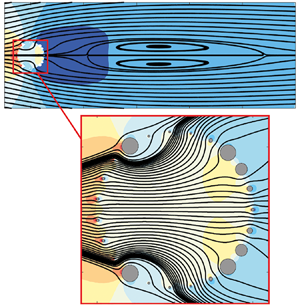
Figure 9. Pressure (a) and viscous stress (b) contributions to the drag following the cylinder surface. The angle $\alpha$ is measured counterclockwise starting from the rear. The colours denote different values of $\mathcal {F}=10^{-4}$ (blue), $\mathcal {F}=5 \times 10^{-3}$ (orange), $\mathcal {F}= 10^{-2}$ (yellow), $\mathcal {F}=5 \times 10^{-2}$ (purple). The slip number is kept fixed to $\mathcal {L}=10^{-4}$. (c)–(e) Streamlines (black bold lines) and iso-contours of the pressure for the steady flow around and through the permeable circular membrane, for different values of $\mathcal {F}$ and $\mathcal {L}=10^{-4}$.

Conversely, as $\mathcal {F}$ is further increased, see the case $\mathcal {F}=5 \times 10^{-2}$, the upstream contribution markedly decreases due to the larger filtrability of the membrane. The substantially higher velocities of the inner flow and the larger filtrability cause a very mild increase of the inner pressure when approaching the downstream part of the membrane. This is again shown also by the streamlines (see figure 9e) which are almost straight in the inner region. Moreover, the larger flow across the downstream part of the membrane decreases the pressure jump between external and internal flows in that area. As a net result, the pressure contribution to drag, in comparison with the impermeable case (here approximated by $\mathcal {F}=10^{-4}$) decreases also in the downstream region. Although the viscous contribution to the drag increases, the total drag decreases because it is quantitatively dominated by the pressure, whose contribution rapidly decays.

In this section, we characterized the morphology of the steady flow, describing the effect of the slip and filtrability numbers. However, not all steady solutions previously described can be observed, as some of them may be unstable with respect to perturbations, thus leading to unsteady configurations. Since conducting time-dependent simulations for every studied case (far beyond $1000$) is a monumental task, we perform a stability analysis, well known to give very accurate predictions of the bifurcations for the case at issue in computational times comparable with the ones of the steady analyses (Chomaz Reference Chomaz2005; Theofilis Reference Theofilis2011). Thus, in the following we study the stability of the steady-flow solution as $\mathcal {L}$ and $\mathcal {F}$ are varied.

3.2. Stability analysis of the steady flow

As mentioned in the previous section, to complete the analysis of the chosen flow configuration, we now establish for which combinations of $(Re,\mathcal {F},\mathcal {L})$ the solution is linearly stable with respect to perturbations and thus likely to be observed. The occurrence of bifurcations of the flow leading to different configurations is studied in the framework of linear stability analysis (Chomaz Reference Chomaz2005; Theofilis Reference Theofilis2011). We consider the flow solution as the superposition of the steady solution denoted as $[\boldsymbol {U}(x,y),P(x,y)]$, outlined in the previous section, and an infinitesimal unsteady perturbation. We thus introduce the following normal mode ansatz:

(3.2a,b)\begin{align} u_i(x,y,t)=U_i(x,y)+\sigma \hat{u}_i(x,y)\exp\left(\lambda t\right), \quad p(x,y,t)=P(x,y) +\sigma \hat{p}(x,y)\exp\left(\lambda t\right), \end{align}

where $\sigma \ll 1$. At $O(1)$ the steady version of the flow equations is obtained, satisfied by $[\boldsymbol {U},P]$, and at $O(\sigma )$ the following system of equations is obtained:

(3.3)\begin{gather} \left. \begin{gathered} \lambda \hat{u}_{i}+ \hat{u}_{j} {\partial}_{j} U_{i}+ U_{j} {\partial}_{j} \hat{u}_{i} ={-}{\partial}_{i} \hat{p}+\frac{1}{Re} {\partial}^{2}_{jj} \hat{u}_{i},\\ {\partial}_{i} \hat{u}_{i} =0, \end{gathered} \right\} \end{gather}

(3.4)\begin{gather} \left. \begin{gathered} \hat{u}_{i}=\hat{u}^+_{i}=\hat{u}^{-}_{i},\\ \hat{u}_{i}=Re\mathcal{M}_{i j} \left(\varSigma_{j k}\left(\hat{p}^-,\hat{\boldsymbol{u}}^-\right)-\varSigma_{j k}\left(\hat{p}^+,\hat{\boldsymbol{u}}^+\right)\right)n_k, \end{gathered} \right\} \end{gather}

together with the homogeneous Dirichlet boundary condition at the inlet $\varGamma _{{in}}$, $\hat {u}_1=\hat {u}_2=0$, and the stress-free condition on the sides $\varGamma _{{lat}}$ and at the outlet $\varGamma _{{out}}$, $(-\hat {p}\delta _{ij}+({1}/{Re})\partial _j \hat {u}_i)n_j=0$.

Equations (3.3) and (3.4), together with the boundary conditions on $\varGamma _{in}$, $\varGamma _{lat}$ and $\varGamma _{out}$, define an eigenfunction problem with, possibly, complex eigenvalues $\lambda =\mathrm {Re}(\lambda )+\mathrm {i}\,\mathrm {Im}(\lambda )$. The real part of the eigenvalue is the growth rate of the global mode, and the imaginary part its angular velocity. We introduce the associated Strouhal number defined as $St={\mathrm {Im}(\lambda )}/{2{\rm \pi} }$. The flow is asymptotically unstable if there exists at least one eigenvalue with positive real part; otherwise it is asymptotically stable. The absence of unstable modes therefore ensures the occurrence of the steady solution, while their presence gives useful information about the emerging unsteady flow configuration.

We turn now to describe the results of the linear stability analysis. The solid case exhibits a Hopf bifurcation at $Re=46.7$ that drives the flow to a state that is periodic in time, characterized by the alternate shedding of vortices, the so-called von Kármán vortex street (Barkley Reference Barkley2006). Ledda et al. (Reference Ledda, Siconolfi, Viola, Gallaire and Camarri2018) showed the suppression of this vortex shedding mode for large enough values of the permeability, in the case of porous rectangular cylinders. A preliminary analysis of the permeable membrane shows that the above-described mode is also the only one that destabilizes the steady wake in the range $10< Re<130$. In figure 10 we report the marginal stability curves (i.e. the locus of points with $\mathrm {Re}(\lambda )=0$) in the $(\mathcal {F},Re)$ plane, for different values of $\mathcal {L}$. The marginal stability curves define a stable and an unstable region in the $(\mathcal {F},Re)$ plane. At low values of $\mathcal {F}$ and $\mathcal {L}$, the critical Reynolds number $Re_{cr}$ for the marginal stability coincides with the solid one, i.e. $Re_{cr}=46.7$. An increase in $\mathcal {L}$ leads to a slight increase in $Re_{cr}$ that reaches a maximum approximately equal to $50$ for $\mathcal {L}=0.02$. For $\mathcal {F}>10^{-3}$ the critical Reynolds number increases. We identify a critical value of $\mathcal {F}=\mathcal {F}_{cr}$ beyond which the steady solution is stable. This value depends on the Reynolds and slip numbers. For fixed $\mathcal {L}$, $\mathcal {F}_{cr}$ initially increases with $Re$, reaches a maximum and decreases. Among all cases, the maximum value $\mathcal {F}_{cr} \approx 1.08 \times 10^{-2}$ is achieved for $\mathcal {L} \approx 10^{-4}$.

Figure 10. Marginal stability curves in the plane $(\mathcal {F},Re)$. Each curve is associated with a different value of slip number $\mathcal {L}=10^{-4}$ (blue), $\mathcal {L}=10^{-3}$ (orange), $\mathcal {L}=10^{-2}$ (yellow), $\mathcal {L}=2\times 10^{-2}$ (purple). The inset shows a zoom in for large values of $\mathcal {F}$. The coloured circles represent the values of the Strouhal number along the marginal stability curve in the region depicted in the inset.

The imaginary part of the eigenvalue well approximates the oscillation frequency of the nonlinear limit cycle in marginal stability conditions (Barkley Reference Barkley2006). In the inset of figure 10, we report the value of the Strouhal number along the marginal stability curve. We do not observe substantial variations in the Strouhal number with respect to the solid case, i.e. $St\approx 0.116$ (Norberg Reference Norberg2003).

In figure 11 we report the spatial distribution of $\mathrm {Re}(\hat {u}_1)$ for two different cases, in figure 11$(a)$ characterized by a recirculation region close to the cylinder and in figure 11$(b)$ characterized by a recirculation region far downstream. In both cases, the unstable mode leads to a vortex shedding similar to that of the solid case, as already anticipated. As the recirculation region moves downstream, the onset of the vortex shedding is displaced downstream and the flow in proximity of the cylinder is almost steady.

Figure 11. Real part of the eigenvector $\hat {u}_1$ associated with the marginally stable eigenvalue for $Re=46.7$, $\mathcal {L}=10^{-2}$ and $\mathcal {F}=10^{-3}$ ($a$) and for $Re=87$, $\mathcal {L}=10^{-4}$ and $\mathcal {F}=1.075\times 10^{-2}$ ($b$). The velocity eigenvectors are normalized by their $L_2$ norm.

The analysis of the stability properties of the steady wake shows the strong stabilization effect of the filtrability number. The marginal stability curves strongly resemble those outlined in Ledda et al. (Reference Ledda, Siconolfi, Viola, Gallaire and Camarri2018,  Reference Ledda, Siconolfi, Viola, Camarri and Gallaire2019). In particular, the vortex shedding is suppressed for large enough values of the filtrability. This similarity is confirmed by the spatial distribution of the unstable mode, which moves downstream with the recirculation region of the steady flow. Indeed, the stability properties of the wake can be related to the extent of the so-called absolute region of instability in a local stability analysis (i.e. performed for the velocity profile at each streamwise location; see Monkewitz (Reference Monkewitz1988) and Giannetti & Luchini (Reference Giannetti and Luchini2007)) that roughly corresponds to the recirculation region. As shown in Ledda et al. (Reference Ledda, Siconolfi, Viola, Gallaire and Camarri2018), there is a critical value of the extent of the recirculation region beyond which the flow becomes unstable. When large values of the filtrability are considered, the recirculation region is small or even absent, and thus the vortex shedding is suppressed. For fixed $\mathcal {F} \approx 10^{-2}$ and $\mathcal {L}$ and increasing $Re$, the recirculation region initially increases and then decreases its dimensions (cf. figure 6). Therefore, the first destabilization and subsequent stabilization for fixed $\mathcal {F}$ and $\mathcal {L}$ are due to the non-monotonic behaviour of the length of the recirculation region with $Re$, which crosses the critical value for the marginal stability twice.

By comparing the marginal stability curve with the drag coefficient, we deduce that the maximum of $C_D$ for the steady flow occurs for a stable configuration for all values of $Re$. Interestingly, a permeable circular membrane exhibits a larger drag than the equivalent solid one, and this maximum occurs when the steady flow is stable.

In the present section, we performed a parametric study under the framework of bifurcation theory in order to exclude the unstable configurations from the variety of steady solutions obtained in § 3.1. In the next section, we propose a methodology to obtain the full-scale design of the structure by fulfilling some objectives on the macroscopic behaviour of the steady flow, under the constraint of stable configuration.

4.1. Choosing the design objective

An important macroscopic property is the drag exerted on the solid structure by the incoming fluid. Several attempts of controlling this integral quantity, defined by (3.1), by permeable surfaces have been carried out, some of them focused on minimizing the drag (Garcia-Mayoral & Jiménez Reference Garcia-Mayoral and Jiménez2011; Abderrahaman-Elena & García-Mayoral Reference Abderrahaman-Elena and García-Mayoral2017; Gómez-de Segura & García-Mayoral Reference Gómez-de Segura and García-Mayoral2019), others investigating the conditions for drag maximization (Cummins et al. Reference Cummins, Viola, Mastropaolo and Nakayama2017,  Reference Cummins, Seale, Macente, Certini, Mastropaolo, Viola and Nakayama2018).

We fix $Re=100$ and we study the variation of $C_D$ with $\mathcal {L}$ and $\mathcal {F}$. In figure 12 we report the iso-contours of $C_D$ on the $(\mathcal {F},\mathcal {L})$ plane. The bold solid line corresponds to the marginal stability boundary for $Re=100$. Among all these possible solutions for the drag coefficient, we select the maximum value of the drag coefficient ($C_D=1.339$), which occurs at $\mathcal {F}=1.25\times 10^{-2}$, $\mathcal {L}=5\times 10^{-3}$ (denoted by $\square$ in figure 12) and in the following is compared with the full-scale simulations. For the sake of completeness, we select three other values of $C_D$ denoted by $\bigcirc ,\triangleright ,\star$ in figure 12, to verify the faithfulness of the homogenized model in the parameters space $(\mathcal {F},\mathcal {L})$ for constant $\mathcal {L}=10^{-4}$. Note that the case denoted with $\star$ is unstable, but we use it as an additional test case owing to the large recirculation region that this configuration exhibits.

Figure 12. Iso-contours of $C_D$ for $Re=100$ in the $(\mathcal {F},\mathcal {L})$ plane. Symbols identify the configurations listed in table 1. The marginal stability curve for the value of $Re$ considered is represented by a bold solid line (all cases on the right-hand side of the curve are stable).

4.2. Linking microscopic geometry to macroscopic properties: elliptical inclusions

We now turn to describe the procedure for the determination of the microscopic geometry based on the macroscopic flow properties identified in the previous subsection. We first perform microscopic simulations in the domain depicted in figure 13$(a)$ (dashed rectangle) whose lengths are non-dimensionalized with the microscopic length $\ell$, so that the results do not depend on the separation-of-scales parameter $\varepsilon ={\ell }/{D}$, according to Zampogna & Gallaire (Reference Zampogna and Gallaire2020). Within this domain, two different microscopic problems need to be solved to calculate $\bar {F}_n$ and $\bar {L}_t$; they read respectively

(4.1)\begin{equation} \left. \begin{gathered} -\partial_{i} Q+\partial_{l l}^{2} F_{i}=0, \quad \text{in}\ \mathbb{F},\\ \partial_{i} F_{i}=0, \quad \text{in }\ \mathbb{F},\\ F_{i}=0, \quad \text{on }\ \partial \mathbb{M}, \\ \varSigma_{n n}\left({Q,\boldsymbol{F}}\right)={-}1, \quad \text{on}\ \mathbb{U}, \\ \varSigma_{n n}\left({Q,\boldsymbol{F}}\right)=0 ,\quad \text{on }\ \mathbb{D},\\ F_{i}, Q, \quad \text{periodic along } \boldsymbol{t}, \end{gathered} \right\} \end{equation}

and

(4.2)\begin{equation} \left. \begin{gathered} -\partial_{i} R+\partial_{l l}^{2} L_{i}=0,\quad \text{in}\ \mathbb{F},\\ \partial_{i} L_{i}=0, \quad \text{in}\ \mathbb{F},\\ L_{i}=0, \quad \text{on}\ \partial \mathbb{M}, \\ \varSigma_{t n}\left({R,\boldsymbol{L}}\right)={-}1, \quad \text{on}\ \mathbb{U}, \\ \varSigma_{t n}\left({R,\boldsymbol{L}}\right)=0, \quad \text{on}\ \mathbb{D},\\ L_{i}, R, \quad \text{periodic along } \boldsymbol{t}, \end{gathered} \right\} \end{equation}

where $i,l=t,n$, i.e. the equations are written in the local frame of reference of the cylinder surface. We refer to figure 13$(a)$ for a definition of $\mathbb {F},\mathbb {M},\mathbb {U}$ and $\mathbb {D}$. In the microscopic problems (4.1) and (4.2) the scalar fields $R$ and $Q$ appear. They relate the value of the pressure on $\varGamma _{{int}}$ to the upward and downward fluid stresses and do not contribute to the determination of the macroscopic flow through the membrane (see Zampogna & Gallaire (Reference Zampogna and Gallaire2020) for a detailed explanation). For the purpose of the present work, we are not directly interested in microscopic fields representing the solution of these problems, but we need only to know the quantities $\bar {F}_n$ and $\bar {L}_t$ which appear in the macroscopic model via (2.9), where the symbol $\bar {\cdot }$ denotes the spatial average used in Zampogna & Gallaire (Reference Zampogna and Gallaire2020), i.e.

(4.3)\begin{equation} {\bar{\cdot} = \lim_{\mathbb{U}\rightarrow\mathbb{D}}\frac{1}{\vert{\mathbb{F}}\cup{\mathbb{M}}\vert}\int_{{\mathbb{F}}}\cdot \, \textrm{d}\kern0.7pt \boldsymbol{x} = \frac{1}{\vert\varGamma_{{int}}^{\mathbb{F}}\cup\varGamma_{{int}}^{\mathbb{M}}\vert}\int_{\varGamma_{{int}}^{\mathbb{F}}}\cdot\, \textrm{d}\kern0.7pt \boldsymbol{x},} \end{equation}

with $\varGamma _{{int}}^{\mathbb {F}}$ and $\varGamma _{{int}}^{\mathbb {M}}$ the fluid and solid parts of $\varGamma _{{int}}$ within the unit cell, as sketched in figure 13$(a)$. The linear problems (4.1) and (4.2) are numerically solved for each couple $(l_t,l_n)$, $0.02< l_t,\,l_n<0.98$ (with a step of 0.01), via their weak formulation implemented in the finite-element solver COMSOL Multiphysics. The spatial discretization is based on the Taylor–Hood (P2-P1) triangular elements for $\boldsymbol {F}$-$\boldsymbol {L}$ and $R$-$Q$, respectively. We refer to Zampogna & Gallaire (Reference Zampogna and Gallaire2020) for further details about the solution of the microscopic problems.

Figure 13. (a) Sketch of the membrane (red dashed line) with a zoom on the microscopic elementary cell used to calculate $\bar {L}_t$ and $\bar {F}_n$. The tangential- and normal-to-interface axes of the solid inclusion are respectively denoted with $l_t$ and $l_n$ and normalized by $\ell$. Iso-contours of $\bar {F}_n={\mathcal {F}}/{\varepsilon }$ (b) and $\bar {L}_t={\mathcal {L}}/{\varepsilon }$ (c) on the plane $(l_t,l_n)$, in logarithmic scale. Blue-to-red colours indicate positive values of $\bar {F}_n$ and $\bar {L}_t$ while grey-scale refers to negative values of $\bar {L}_t$. The lines identify the iso-contours of the possible couples $(l_n,l_t)$ whose symbols correspond to different couples $(\mathcal {F},\mathcal {L})$ of figure 12. Each point on those lines is a good candidate to realize the desired value of $\mathcal {F}$ and $\mathcal {L}$, upon adjustment of the value of $\varepsilon$. The selected values of $l_t$ and $l_n$ are labelled with white arrows for each case.

After averaging the solution of the microscopic problems, we deduce $\bar {F}_n$ and $\bar {L}_t$, whose iso-contours are reported in figure 13(b,c) as functions of the two axes $l_n$ and $l_t$.

The parameters $\mathcal {F}$ and $\mathcal {L}$ are then calculated by a renormalization of $\bar {F}_n$ and $\bar {L}_t$ with respect to the macroscopic length scale, i.e.

(4.4a,b)\begin{equation} \mathcal{F}=\varepsilon\bar{F}_n \quad\text{and}\quad \mathcal{L}=\varepsilon\bar{L}_t. \end{equation}

While in a direct approach the parameters defining the full-scale geometry $l_t$, $l_n$ and $\varepsilon$ are given and the corresponding filtrability and slip numbers are evaluated, in the inverse procedure they need to be determined based on the choice of a given property that has to be satisfied by the fluid flow. Actually, there is no one-to-one relation linking $\mathcal {F}$ and $\mathcal {L}$ to the microscopic geometry. Once filtrability and slip are chosen, one has potentially full freedom in the choice of the microscopic structure. This choice is essentially related to the geometrical shape of the microscopic inclusions, in this case ellipsoidal ones with variable axes, and to their relative size with respect to the macroscopic length, as outlined in figure 13(b,c), where several configurations satisfy the desired values of $\mathcal {F}$ and $\mathcal {L}$, each one associated with a value of $\varepsilon$. For the sake of clarity we list the steps to follow in order to determine these geometrical parameters which allow us to define the microscopic geometry of the permeable shell:

1. (i) According to the previous subsection, we identify a pair $(\mathcal {F},\mathcal {L})=(\mathcal {F}^*,\mathcal {L}^*)$ of interest.

2. (ii) We find in the $l_t$–$l_n$ plane the possible pairs of $(l_t,l_n)$ that can give the correct set $(\mathcal {F}^*,\mathcal {L}^*)$. These values are found by evaluating the ratio ${\mathcal {F}^*}/{\mathcal {L}^*}$, which does not depend on $\varepsilon$ (since $F_n$ and $L_t$ are proportional to $\varepsilon$). The potential values of $l_n$ and $l_t$ are those associated with the black solid lines in figure 13(b,c), which realize $C_D^*$ upon renormalization by the proper value of $\varepsilon$ that is still undetermined.

3. (iii) Among the potential candidates, the final value of $\varepsilon$ and thus the values of $(l_t,l_n)$ can be chosen based on other constraints (like, for instance, the minimization of microscopic anisotropy, i.e. $l_t \approx l_n$, the minimization of $\varepsilon$ or the satisfaction of geometrical properties of the medium like the fluid-to-solid ratio).

4. (iv) Once the value of $\varepsilon$ is selected, there is only one couple $(l_t,l_n)$ that satisfies the macroscopic values of ${\mathcal {F}}^*={\varepsilon }\bar {F}_n$ and ${\mathcal {L}^*}={\varepsilon }\bar {L}_t$. We then deduce $\bar {F}_n$ and $\bar {L}_t$, and eventually $l_t$ and $l_n$.

The values of $\varepsilon$, $l_t$ and $l_n$ are deduced for each case highlighted by the symbols in figure 12. Table 1 shows the values found for each case, corresponding to the white pointers in figure 13$(b)$. For the cases denoted by $\bigcirc$, $\triangleright$ and $\square$ the values of $(l_t,l_n)$ have been chosen so as to obtain a value of $\varepsilon$ of order $10^{-1}$, while for the case $\star$ the value of $(l_t,l_n)$ guarantees minimal anisotropy with the constraint $\varepsilon \leq 0.045$.

Table 1. Relevant geometrical and physical parameters for the cases chosen in figure 12; $N$ indicates the number of inclusions forming the membrane, the superscript $^{EQ}$ denotes quantities calculated using model (2.7) on $\varGamma _{int}$ while the absence of superscript denotes quantities evaluated from the full-scale solution.

The final full-scale geometries are thus obtained by distributing the inclusions along the membrane centreline $\varGamma _{int}$, with a constant angular distance among them given by $\Delta \phi ={2{\rm \pi} }\lfloor {\varepsilon }/{{\rm \pi} }\rfloor$, with $\lfloor \cdot \rfloor$ the integer part in order to have an integer number of inclusions along the cylindrical shell. Two examples of microscopic geometries obtained are depicted in figure 14, where $69$ and $32$ inclusions are employed. Once the full-scale geometry is built, the reliability of the inverse procedure is verified as explained in the next section.

Figure 14. Comparison between full-scale and equivalent model for cases $\star$ and $\square$ identified in figure 12. The microscopic geometry forming the cylindrical shell, sketched for each case in the grey insets on the left, is the result of the inverse procedure explained in § 4.2. (a,d) Flow streamlines for the full-scale case (black dashed lines) and for the macroscopic model (blue solid lines). (b,c,e,f) Horizontal and vertical velocities $U_1$ and $U_2$ sampled on the cylindrical shell using the angle $\alpha$ measured counterclockwise starting from the rear. Dashed lines represent the full-scale model, blue lines the macroscopic model and red stars the average of the full-scale model, calculated applying a discrete version of the integral in (4.3), based on a 1-point Gaussian rule, to the velocity profile in each microscopic elementary cell forming the membrane. Numerical values of $\epsilon$, $\mathcal {F}$, $\mathcal {L}$ and other representative values of the fluid flow ($C_D$, $X_R$, $L_R$) are listed in table 1 for each case.

4.3. Comparison between homogenized and full-scale results

We verify the faithfulness of the homogenization approach and the subsequent retrieval of the microscopic geometry by comparing the results obtained using the equivalent model with the feature-resolved flow past the full-scale permeable shell. To deduce the full-scale flow, the Navier–Stokes equations are solved in the full-scale domain, where each solid inclusion forming the membrane is explicitly taken into account in the fluid domain and thus in the mesh. The full-scale problem is solved by the finite-element solver COMSOL Multiphysics, using the same numerical set-up as for the macroscopic flow solution. In order to have spatially converged results, mesh M1 (see Appendix A) has been modified in the vicinity of the full-scale structure. A circular refinement region of diameter 1.1$L$ has been added with a resolution chosen in order to guarantee at least $10^{2}$ cells between two adjacent solid inclusions whose boundary has been discretized using at least $50$ segments. The boundary conditions on $\varGamma _{in}$, $\varGamma _{out}$ and $\varGamma _{lat}$ are the same as in the case of the macroscopic model (2.7), while we impose a no-slip condition on the walls of each microscopic inclusion, i.e. $u_i|_{\varGamma _{\partial \mathbb {M}}}=0$.

In figure 14 we report two sample comparisons of the flow fields obtained with the homogenized model and with the full-scale simulations (cases $\star$ and $\square$ identified in figure 12), together with the velocities at the membrane. In both cases, we observe a good agreement between the two approaches, with an error on the velocities along the membrane of the order of $\varepsilon$, as expected.

In table 1 we report the reference values ($C_D$, $L_R$, $X_R$) for all cases identified in figure 12. Also in this case, we observe an overall good agreement, even for extremely large values of $\varepsilon$, which are far beyond the rigorous domain of validity of the theory. Only for the case denoted by $\bigcirc$ are the differences in $C_D$ non-negligible, suggesting that a maximum value of $\varepsilon$ beyond which macroscopic model (2.7) is no more applicable lies between $10^{-1}$ and $3.5\times 10^{-1}$. A complete validation also requires the comparison of the stability properties of the flow between homogenized model and full-scale simulations, reported in figure 15. We observe a good agreement between the spectra, and in particular the leading eigenvalues are well described by the homogenized model. Considering the one with largest real part, the relative errors on the absolute value are $0.25\,\%$ for the case $\star$ ($\lambda =0.076+0.64\mathrm {i}$) and $0.6\,\%$ for the case $\square$ ($\lambda =-0.039+0.72\mathrm {i}$). We finally stress the importance of the validation described above, since it constitutes a strong proof of the faithfulness of the model developed in Zampogna & Gallaire (Reference Zampogna and Gallaire2020) in the case of flows with non-negligible macroscopic inertia.

Figure 15. (a,b) Comparison between the homogenized and full-scale results of the stability analysis. The crosses and the circles denote the eigenvalues obtained from the full-scale structure and from the homogenized model, respectively, for the two reported cases.

In this section, we outlined a method for the geometrical reconstruction of the microscopic geometry based on the macroscopic properties of the membrane, thus concluding the first branch of the scheme described by figure 3. We note that the homogenized model, combined with the stability analysis technique, allows us to perform a parametric study spanning a very large range of possible geometries with extremely fast outputs. The flow through the resulting microscopic structure shows a good agreement with the homogenized model, thus giving confidence in the parametric study carried out in § 3. We verified the validity of the homogenized model through permeable membranes for Reynolds numbers of the order of $10^2$. The error on the final solution is of order $\varepsilon$, thus degrading the solution when extremely large values of $\varepsilon$ are considered. Nevertheless, the homogenized model gives also in these cases fairly reasonable results that can be used as guidelines in a first parametric study, before optimizing the resulting microscopic structure.

The previous analysis was focused on membranes with monodisperse and identical microscopic inclusions along the centreline of the membrane. In the following, we analyse the opportunity to exploit membranes of variable permeability by employing a Lagrangian-based optimization, i.e. we focus on the second branch of the diagram of figure 3, in the inverse procedure part.

5.1. Sensitivity with respect to variations of the slip and filtrability numbers

In this section, we introduce the theoretical framework for the adjoint-based optimization of the structure of the membrane. We recall that, at the interface, we denote with superscript plus sign the variables evaluated in the inner part of the cylinder and with superscript minus sign those evaluated in the outer part. Any small modification $\delta \mathcal {M}_{ij}$ of the tensor component $\mathcal {M}_{ij}$ (i.e. variations of $\mathcal {F}$ or $\mathcal {L}$) induces a perturbation $(\delta \boldsymbol {u}, \delta p)$ on the flow field such that $(\boldsymbol {u}, p)=(\boldsymbol {U}+\delta \boldsymbol {u},P+\delta p)$. The drag coefficient, i.e. the objective in the Lagrangian framework, is written as follows:

(5.1)\begin{equation} C_D=2 \oint_{\varGamma_{{cyl}}}\left(\varSigma_{jk}\left(p^-, \boldsymbol{u}^-\right)-\varSigma_{jk}\left(p^+, \boldsymbol{u}^+\right) \right) {n}_k {\delta}_{1j}\,\mathrm{d} \varGamma. \end{equation}

The modification $\delta \mathcal {M}_{ij}$ thus perturbs the drag by $\delta C_D$ according to

(5.2)\begin{align} \delta C_D=2 \oint_{\varGamma_{{cyl}}}\left(\varSigma_{jk}\left(\delta p^-, \delta \boldsymbol{u}^-\right)-\varSigma_{jk}\left(\delta p^+, \delta \boldsymbol{u}^+\right) \right) {n}_k {\delta}_{1j} \,\mathrm{d} \varGamma=\oint_{\varGamma_{cyl}} \boldsymbol{\nabla}_{\mathcal{M}_{ij}} C_D \delta \mathcal{M}_{ij}\,\mathrm{d}\varGamma. \end{align}

The quantities $(\delta \boldsymbol {u}^\pm , \delta p^\pm )$ are the solution of (B3) reported in Appendix B, where a formal derivation of the sensitivity functions (i.e. the functions describing the variations of the objective $C_D$ with respect to the control variable $\mathcal {F}$ and $\mathcal {L}$) is carried out. In the Lagrangian framework, the sensitivities of the drag coefficient with respect to variations of $\mathcal {L}$ and $\mathcal {F}$ are

(5.3)\begin{equation} \boldsymbol{\nabla}_{\mathcal{F}} C_D={-}Re u_i^{{{\dagger}}{{\dagger}}} \left(\varSigma_{jk}\left(P^-, \boldsymbol{U}^-\right)-\varSigma_{jk}\left(P^+, \boldsymbol{U}^+\right) \right) n_i n_j{n}_k \end{equation}

and

(5.4)\begin{equation} \boldsymbol{\nabla}_{\mathcal{L}} C_D=Re u_i^{{{\dagger}}{{\dagger}}} \left(\varSigma_{jk}\left(P^-, \boldsymbol{U}^-\right)-\varSigma_{jk}\left(P^+, \boldsymbol{U}^+\right) \right) t_it_j {n}_k, \end{equation}

where the Lagrange multipliers $(\boldsymbol {u}^{{\dagger} }, p^{{\dagger} }, \boldsymbol {u}^{{\dagger} {\dagger} })$, also called adjoint variables, are the solution of the following linear problem:

(5.5) \begin{equation} \left. \begin{gathered} {\partial}_{i} {u}_{i}^{\dagger}=0, \quad {u}_{j}^{\dagger} {\partial}_{i} U_{j}- U_{j} {\partial}_{j} {u}_{i}^{\dagger}={\partial}_{i} {p}^{\dagger}{+}\frac{1}{Re} {\partial}^{2}_{jj} {u}_{i}^{\dagger} \quad \text{ in } \varOmega,\\ \left(\varSigma_{ik}\left({-}p^{{{\dagger}}{-}}, \boldsymbol{u}^{{{\dagger}}{-}}\right)-\varSigma_{ik}\left({-}p^{{{\dagger}}{+}}, \boldsymbol{u}^{{{\dagger}}{+}}\right)\right) {n}_k-u_i^{{{\dagger}}{{\dagger}}}={0} \quad \text{ on } \varGamma_{{int }}, \\ u_i^{{{\dagger}}{+}}=u_i^{{{\dagger}}{-}} \quad \text{ on } \varGamma_{{int}} \end{gathered} \right\} \end{equation}

and

(5.6)\begin{equation} u_i^{{{\dagger}}{{\dagger}}}=Re^{{-}1} \mathcal{M}_{ji}^{{-}1}\left(u_j^{{{\dagger}}{-}}-2{\delta}_{1j}\right) \quad \text{ on } \varGamma_{{int}}, \end{equation}

together with the adjoint boundary conditions ${u}_{i}^{{\dagger} }=0$ at the inflow, $\partial _{2} {u}_{1 }^{{\dagger} }=u_{2}^{{\dagger} }=0$ at the transverse boundaries and $\varSigma _{ik}(-p^{{\dagger} }, \boldsymbol {u}^{{\dagger} }) {n}_k+{u}_k {n}_k {u}_i^{{\dagger} }=0$ at the outflow. At this point, it is clear that in order to understand how the control variables $\mathcal {F}$ and $\mathcal {L}$ influence the objective function $C_D$ via (5.3), (5.4), the linear problem (5.5) has to be solved, without the necessity of explicitly evaluating the perturbed state $(\boldsymbol {u}, p)=(\boldsymbol {U}+\delta \boldsymbol {u},P+\delta p)$. The linear adjoint problem presents an advantage in terms of computational time with respect to the nonlinear problem for $(\boldsymbol {u},p)$, and is suitable for a gradient-based optimization with a progressive update of the distribution of the membrane properties.

In figure 16$(a)$ we report the variation of the drag coefficient with $\mathcal {F}$, for fixed $\mathcal {L}=5\times 10^{-3}$ (black dots), together with the prediction given by the sensitivity analysis (solid lines), close to the configuration of maximum $C_D$ identified by the $\square$ symbol in figure 12. Note that, at this stage, we keep $\mathcal {F}$ uniform along the membrane. A good agreement is observed, in the vicinity of the points where the sensitivity is evaluated, i.e. $\delta \mathcal {F} \approx 0.01 \mathcal {F}$. The deviation becomes more important for variations larger than $\delta \mathcal {F} \approx 0.01 \mathcal {F}$, showing a rather strong effect of nonlinearities close to the point of the maximum drag coefficient. In figure 16$(b)$ we show the distribution of sensitivity along the upper part of the cylinder, for three cases. The distribution exhibits a non-monotonic behaviour, with positive values in the front and in the middle of the membrane, and negative values close to the rear of the cylinder.

Figure 16. $(a)$ Variation of the drag coefficient with $\mathcal {F}$, for $\mathcal {L}=5 \times 10^{-3}$, directly evaluated from macroscopic model (2.6), (2.7) (black circles) and predictions of the gradient via the sensitivity approach (coloured lines) carried out around the configurations identified by coloured circles. $(b)$ Distribution of sensitivity with respect to $\mathcal {F}$ along the $y>0$ part of the cylinder, i.e. $0<\alpha <{\rm \pi}$, for the configurations denoted with colours in $(a)$.

The same analysis is performed for uniform variations of $\mathcal {L}$ (figure 17). In this case, we observe a monotonic behaviour, and the variations of the drag coefficient with $\mathcal {L}$ are considerably smaller than those observed when varying $\mathcal {F}$. The distribution, at low values of $\mathcal {L} \approx 5 \times 10^{-3}$, shows a peak at $\alpha \approx 130^\circ$, which decreases with $\mathcal {L}$, and is negative in the other regions of the membrane.

Figure 17. $(a)$ Variation of the drag coefficient with $\mathcal {L}$, for $\mathcal {F}=0.03$, directly evaluated from macroscopic model (2.6), (2.7) (black circles) and predictions of the gradient via the sensitivity approach (coloured lines) carried out around the corresponding coloured circles. $(b)$ Distribution of sensitivity with respect to $\mathcal {L}$ along the $y>0$ part of the cylinder, $0<\alpha <{\rm \pi}$.

In this section, we derived the sensitivity of the drag coefficient with respect to variations of $\mathcal {F}$ and $\mathcal {L}$. In the following, we exploit the sensitivity analysis to introduce a gradient-based optimization for the geometry of the membrane, when both the filtrability and slip numbers are varied together, so as to find the optimal distribution of $\mathcal {F}$ and $\mathcal {L}$ to maximize the drag coefficient.

5.2. Optimal distribution of the properties of the membrane

The sensitivity functions found in the previous section are used here to obtain the optimal distributions of $\mathcal {F}$ and $\mathcal {L}$ that maximize the drag coefficient. The starting profiles of $\mathcal {F}$ and $\mathcal {L}$ for the gradient-based optimization are uniform. We chose different values of the initial guess, among which $\mathcal {F}^{(0)}=1.25\times 10^{-2}$ and $\mathcal {L}^{(0)}=5\times 10^{-3}$, i.e. the values that maximize $C_D$ when the permeable membrane is formed by a repetition of a single microscopic inclusion (case denoted by the $\square$ symbol in figure 12). We implement a gradient-ascent iterative procedure, using as initial guess $\mathcal {F}^{(0)}$ and $\mathcal {L}^{(0)}$. At each iteration $(i)$, the values of the gradients $\boldsymbol {\nabla }_\mathcal {F}^{(i)} C_D$ and $\boldsymbol {\nabla }_\mathcal {L}^{(i)} C_D$ are evaluated by the adjoint analysis proposed above. We thus update the distribution of $\mathcal {F}$ and $\mathcal {L}$ in the direction of the gradient as follows:

(5.7a,b)\begin{equation} \mathcal{F}^{(i+1)}=\mathcal{F}^{(i)} + \boldsymbol{\nabla}_\mathcal{F}^{(i)} C_D\delta \mathcal{F} \quad \text{and} \quad \mathcal{L}^{(i+1)}=\mathcal{L}^{(i)} + \boldsymbol{\nabla}_\mathcal{L}^{(i)} C_D\delta \mathcal{L}, \end{equation}

with fixed step sizes $\delta \mathcal {F}=10^{-2}\mathcal {F}^{(0)}$ and $\delta \mathcal {L}=10^{-2}\mathcal {L}^{(0)}$. During the optimization procedure, the values of $\mathcal {F}$ and $\mathcal {L}$ have to remain strictly positive, to avoid non-physical values. Besides, too small or too large values jeopardize the inverse procedure, since large differences in the dimensions of the microscopic inclusions are difficult to handle without considering large values of the parameter $\varepsilon$, which degrade the accuracy of the homogenized model. Typical procedures to regularize the problem are based on the introduction of auxiliary variables to transform the inequality conditions into equality ones (Schulze & Sesterhenn Reference Schulze and Sesterhenn2013), or on the truncation of the gradient when the threshold values are reached (Lin Reference Lin2007). In this work, for the sake of simplicity, we apply the latter procedure and we restrict the research of the optimal profiles to the intervals $10^{-3}<\mathcal {F},\,\mathcal {L}<1.5\times 10^{-2}$. At each iteration, values of $\mathcal {F}$ or $\mathcal {L}$ larger (smaller) than the threshold value, due to an increase (decrease) along the gradient direction, are imposed to be equal to the threshold value. The iterative procedure is stopped when the relative difference between two successive evaluations of the drag coefficient is less than $10^{-4}$.

In figure 18 we report the optimal distribution of $\mathcal {F}$ and $\mathcal {L}$ along the semi-cylinder found via the iterative algorithm, for the optimization with both $\mathcal {F}$ and $\mathcal {L}$, with different initial guesses. Note that, depending on the initial value, a different number of iterations is needed to achieve convergence. While the final distribution of $\mathcal {F}$ does not show significant variations with the initial guess, the profiles of $\mathcal {L}$ are different. In the rear part, $0<\alpha <{\rm \pi} /2$, $\mathcal {L}$ remains constant and equal to the initial value. For $\alpha \approx {\rm \pi}/2$, all distributions collapse to the lower threshold value, and in the front part they assume different values. However, the effect of the slip number on the final value of the drag coefficient (figure 19$a$) is small and the differences are below $0.5\,\%$. Therefore, the effect of the filtrability is predominant and the optimal distribution of $\mathcal {F}$ is weakly influenced by $\mathcal {L}$. We thus consider the case in which the slip number is kept fixed, while the optimization is performed only on $\mathcal {F}$. The resulting distribution (red dashed line in figure 18$a$) is very similar to the other ones optimized with respect to both $\mathcal {F}$ and $\mathcal {L}$. Both approaches converge to a similar value of $C_D$ (figure 19$b$), which is $\approx 6\,\%$ larger than the maximum drag obtained with uniform membrane properties. We therefore conclude that the optimization procedure leads to significantly larger values of $C_D$, in which the effect of the filtrability is predominant, with a weak dependence on the initial guess.

Figure 18. Results from the gradient-based optimization. Final distribution of $(a)$ $\mathcal {F}$ and $(b)$ $\mathcal {L}$, when both $\mathcal {F}$ and $\mathcal {L}$ are optimized for different initial guesses (coloured lines) and when only variations of $\mathcal {F}$ are considered with initial guess $\mathcal {F}^{(0)}=0.0125$ and $\mathcal {L}^{(0)}=0.005$ (red dashed line). The various initial guesses are $\mathcal {F}^{(0)}=0.0125$ and $\mathcal {L}^{(0)}=0.005$ (blue), $\mathcal {F}^{(0)}=0.005$ and $\mathcal {L}^{(0)}=0.0125$ (orange), $\mathcal {F}^{(0)}=0.0025$ and $\mathcal {L}^{(0)}=0.0025$ (yellow), $\mathcal {F}^{(0)}=0.005$ and $\mathcal {L}^{(0)}=0.005$ (purple), $\mathcal {F}^{(0)}=0.01$, $\mathcal {L}^{(0)}=0.01$ (green).

Figure 19. $(a)$ Variation of the drag coefficient during the optimization procedure, for different initial guesses, as a function of the iteration number rescaled by the total number of iterations required to reach convergence. $(b)$ Variation of the drag coefficient during the iterative procedure of the gradient-based optimization, when both $\mathcal {F}$ and $\mathcal {L}$ (blue dots) and only $\mathcal {F}$ (orange dots) are varied, with initial guess $\mathcal {F}^{(0)}=0.0125$ and $\mathcal {L}^{(0)}=0.005$. In the insets, we report the distributions of $\mathcal {F}$ for different iterations, the horizontal and vertical axes of the insets corresponding to $0<\alpha <{\rm \pi}$ and $0<\mathcal {F}<1.55\times 10^{-2}$, respectively.

The increase of drag in the optimal configuration can be related to the previous observations in the case of constant filtrability. The optimization procedure tends to increase the filtrability in the front part ($\alpha \approx {\rm \pi}$) of the cylinder and at $\alpha \approx {\rm \pi}/2$, while it tends to decrease it at $\alpha \approx {\rm \pi}/4$ and $\alpha \approx (3/4){\rm \pi}$. Compared with the constant filtrability case, the curvature of the streamlines is enhanced, thus leading to a more marked recompression in the inner part of the downstream portion of the membrane. This effect, leading to an increase of global drag, is enhanced in the optimal configuration since the flow is more constrained to pass through the front and the streamlines leave the cylinder through a narrower region, at $\alpha \approx {\rm \pi}/2$, owing to the large values of filtrability in these regions. This constraint further magnifies the effects of the inner pressure gradients presented in the constant properties case. The analysis of the distributions of slip number shows that the drag is not influenced by variations of slip in the rear part of the cylinder.

In this section, we performed an adjoint-based optimization of the flow with respect to the drag. The typical computational time for one step of the optimization is equivalent to that of a steady calculation of the nonlinear Navier–Stokes equations, i.e. around one minute for a common laptop computer. Since on average 30–60 iterations were needed to achieve convergence, with the presented simple algorithm, one optimization lasts for 30–60 minutes. The decoupling between microscopic properties and macroscopic effects on the flow allows one to move from a generic shape optimization problem to an optimization problem for the two scalar distributions $\mathcal {F}(\alpha )$ and $\mathcal {L}(\alpha )$, making the optimization procedure straightforward to implement compared with a full-scale case. Once the distribution of membrane properties is known, the inverse procedure has to be applied to choose the microscopic structure. In the following, we aim at retrieving an optimal full-scale structure of the membrane starting from the optimal profile of $\mathcal {F}$ found in the present section.

6.1. Application of the effective stress jump model to the case of membranes with fast-varying microscopic geometry

The easiest way to compute the microscopic tensors within the homogenization framework is to assume that the solid structure consists of a periodic repetition of a given unit cell (for a review, see Hornung (Reference Hornung1997)). To relax this assumption one may assume that the variations of the microscopic structure are slow (e.g. Dalwadi, Bruna & Griffiths Reference Dalwadi, Bruna and Griffiths2016) and hence solve the microscopic periodic problems (4.1) and (4.2) over each periodic unit cell and then compute the effective macroscopic tensors by averaging the microscopic solution over each cell. In the context of the present work, since fast variations of $\mathcal {F}$ and $\mathcal {L}$ can be noticed in the optimal distributions of figure 18, we need a model to link the effective properties to the microscopic geometry, without any assumption about the nature of the variations of the inclusions along the membrane. The macroscopic model of Zampogna & Gallaire (Reference Zampogna and Gallaire2020) is adapted here so as to describe this case when the following hypotheses are valid:

1. (i) the permeable shell is the surface of a rotational body, whose radius is $R$;

2. (ii) the constraint $\ell /D\ll 1$ is still valid.

Under such assumptions, the macroscopic curvature is neglected in the microscopic domain as also done in Zampogna & Gallaire (Reference Zampogna and Gallaire2020) and the microscopic problems (4.1) and (4.2) are solved in the entire cylindrical shell, $\mathbb {F}_{tot}$, sketched in figure 20$(b)$, defined as

(6.1)\begin{equation} \mathbb{F}_{tot}=\cup_{i=1}^{N}\mathbb{F}_i, \end{equation}

where $\mathbb {F}_i$ is the fluid domain within the $i$th unit cell sketched in figure 20$(b)$ and $N$ the total number of solid inclusions on the shell. On the left and right sides of $\mathbb {F}_{tot}$, we impose periodic boundary conditions as we are dealing with the surface of a rotational body. With these modifications, i.e. solving the microscopic problems (4.1) and (4.2) over $\mathbb {F}_{tot}$ instead of over each $\mathbb {F}_{i}$, the assumption of slow variations of the microscopic geometry is superfluous and a fast-varying microscopic geometry can be studied and associated with the optimal profile of $\mathcal {F}$ found in the previous subsection. To validate the model, we first calculate the microscopic quantities associated with two different distributions of solid inclusions along the membrane, D1 and D2. They represent an example of slow-varying (D1) and fast-varying (D2) microscopic geometries (see Appendix C). The distribution D1 is represented in the Cartesian frame of reference in figure 20$(a)$ and in the local frame of reference of the cylinder in figure 20$(b)$. The values of $\mathcal {F}$ and $\mathcal {L}$ for distributions D1 and D2 are shown in figures 21$(a{,}b)$ and 21$(c{,}d)$, respectively. While blue stars represent the values extracted from the solutions computed within $\mathbb {F}_{tot}$ by averaging over each unit cell, the light-blue circles represent the values of $\mathcal {F}$ and $\mathcal {L}$ deduced by classical calculations over each periodic unit cell $\mathbb {F}_{i}$. In the case of slow variations of the microscopic structure, the periodic problems (4.1) and (4.2) over the unit cell provide acceptable results for the effective tensors. Conversely, the important discrepancies between the blue and light-blue profiles represented in figure 21(c,d) show that fast variations of the microscopic geometries affect in a relevant way the values of the effective quantities $\mathcal {F}$ and $\mathcal {L}$ and microscopic problems (4.1) and (4.2) have to be computed over the entire microscopic domain $\mathbb {F}_{tot}$.

Figure 20. $(a)$ Example of a cylindrical shell formed by variable microscopic inclusions, corresponding to distribution D1 in Appendix C. $(b)$ Sketch of the microscopic domain, $\mathbb {F}_{tot}$, built by ‘unrolling’ the cylindrical shell (red and blue unit cells correspond to their ‘rolled’ counterpart in $a$). In order to deduce averaged profiles of $F_n$ and $L_t$, the solution is averaged within each cell over the green dashed line.

Figure 21. Values of $\mathcal {F}$ and $\mathcal {L}$ along $\mathbb {F}_{tot}$ (blue stars) and corresponding values computed within each cell $\mathbb {F}_{i}$ (light-blue circles) for distributions D1 (a,b) and D2 (c,d) described in Appendix C.

The last statement is supported by the comparison between the full-scale and the equivalent model that can be done once the effective values of $\mathcal {F}$ and $\mathcal {L}$ have been found. As shown in figure 22, the macroscopic velocities evaluated over the membrane are in perfect agreement with the full-scale profile for the case D1 of slow-varying geometries. The drag coefficient computed from the equivalent solution, $C_D^{EQ}$, is equal to 1.225, with a relative error with respect to the full-scale solution of $\approx 1.5\,\%$, in the order of the approximation. No substantial differences are noticed using the values of the effective tensor extracted from $\mathbb {F}_{tot}$ or from each periodic unit cell $\mathbb {F}_{i}$. In contrast, when distribution D2 is considered (figure 22c,d), the use of the effective tensor calculated within $\mathbb {F}_{tot}$ allows us to markedly reduce the error between the full-scale simulation and the macroscopic model.

Figure 22. Comparison between the full-scale solution and the macroscopic model for distributions D1 (a,b) and D2 (c,d). All quantities are evaluated over the equivalent membrane $\varGamma _{int}$. Dashed lines represent the full-scale model, blue lines the macroscopic model where the values of the effective tensors have been calculated in $\mathbb {F}_{tot}$, light-blue dot-dashed lines correspond to the macroscopic model where the values of the effective tensors have been calculated in each periodic unit cell $\mathbb {F}_{i}$ and red stars represent the average of the full-scale model.

6.2. Retrieving the full-scale microscopic geometry from the optimal $\mathcal {F}$–$\mathcal {L}$ profiles

In the previous subsection we showed that the effective stress jump condition of Zampogna & Gallaire (Reference Zampogna and Gallaire2020) is reliable also in the case of fast-varying microscopic geometries when the adequate precautions described above are taken into account to formulate microscopic problems (4.1) and (4.2). We thus apply it to link the optimal distributions of effective filtrability and slip profiles found in § 5.2 to a distribution of microscopic solid inclusions in order to design an optimal cylindrical membrane for drag maximization. For the sake of simplicity, we consider the case in which the optimization procedure is performed only on the value of $\mathcal {F}$, letting $\mathcal {L}$ vary according to the microscopic calculations. This allows us to focus our attention only on circular (rather than elliptical) inclusions of variable radius. As a consequence, the profile of $\mathcal {L}$ is unequivocally defined once the $\mathcal {F}$ profile is retrieved. This simplifying assumption has a marginal effect on the resulting optimal drag since the latter is only weakly affected by $\mathcal {L}$. Nevertheless, the following procedure can be straightforwardly generalized to variable distributions of both $\mathcal {F}$ and $\mathcal {L}$, by considering for instance elliptical inclusions as in § 4.2. The numerical implementation is based on a bisection method (see Appendix C), where at each iteration the value of the radius of each inclusion is adjusted so as to reach the aimed values of $\mathcal {F}$ up to a relative tolerance of $1\,\%$. For the iterative procedure to be well defined, an initial guess has to be made. A good candidate is the value of $\mathcal {F}$ given by the case of perfectly periodic microstructures. The separation-of-scales parameter $\varepsilon$ is a free parameter and has to be chosen to unequivocally define the radius of the solid inclusions. The resulting distributions are sketched in figure 23 for two different values of $\varepsilon =0.1369$ and $0.0667$, corresponding to 23 and 47 solid inclusions over the cylinder, respectively. We reconstruct the continuous $\mathcal {F}$ and $\mathcal {L}$ profiles via a piecewise-cubic interpolation (black dashed lines in figure 23) of the piecewise-constant values obtained from the solution of the microscopic problems averaged in each unit cell (red squares); however, we verified that the following results were not affected by a different choice of the interpolation. As a last check, we perform macroscopic and full-scale simulations in order to (i) confirm the validity of the model in this case and (ii) check that the full-scale geometry actually maximizes the drag coefficient, as predicted in the Lagrangian-based optimization procedure. Figures 24 and 25 provide qualitative and quantitative information about the flow past the two retrieved full-scale optimal structures. According to figures 24(a–c) and 25(a–c), for both values of $\varepsilon$ the full-scale solution reproduces well the behaviour and properties of the macroscopic flow calculated using the optimal profile of $\mathcal {F}$. The drag coefficients calculated over the two full-scale structures are $C_D^{\varepsilon =0.1369}=1.427$ and $C_D^{\varepsilon =0.0667}=1.412$, while the corresponding one estimated by the macroscopic model is equal to 1.414, exhibiting an error of about $1\,\%$ in the worst case. The variability of the microscopic inclusions is shown in figures 24(d–f) and 25(d–f), where a focus on the pressure and velocity fields across the cylindrical shell reveals the presence of local microscopic flow structures that become less and less important as $\varepsilon$ decreases. We refer to Appendix C for the geometrical data used to build each full-scale structure and for their visualization.

Figure 23. Variation of the optimal $\mathcal {F}$ profile with $\alpha$. Blue lines correspond to the values of $\mathcal {F}$ found in § 5.2 while red squares to the values of $\mathcal {F}$ reconstructed from the microscopic problems in $\mathbb {F}_{tot}$. Black dashed lines correspond to the profiles reconstructed via a piecewise cubic interpolation of the red-square profile. (a) A total of 23 inclusions have been placed on the cylindrical shell ($\epsilon =0.1369$); (b) 47 inclusions have been used ($\varepsilon =0.0667$). A larger number of inclusions allows us to better reconstruct the $\mathcal {F}$ profile.

Figure 24. Flow past the optimal cylindrical structure deduced from the profile of $\mathcal {F}$ computed in § 5.2. A total of 23 solid inclusions (sketched in dark grey in d–f) have been placed on the cylinder leading to a value of $\varepsilon$ equal to $0.137$. (a–c) Comparison between full-scale and macroscopic solution. (a) The flow streamlines for the full-scale simulation (black lines) and for the macroscopic model (blue lines). (b,c) The horizontal and vertical velocities over $\varGamma _{int}$. Black dashed lines represent the full-scale solution, blue lines the macroscopic model, where $\mathcal {F}$ and $\mathcal {L}$ are evaluated using the reconstructed profiles (see figure 23), and red stars the averaged full-scale profile. Iso-contours of pressure (d), horizontal velocity (e) and vertical velocity (f) around the cylindrical shell. In (d) also flow streamlines within the shell have been represented to better appreciate the flow behaviour.

Figure 25. Same as figure 24 for a total number of 47 solid inclusions on the cylinder, leading to $\varepsilon =0.066$.

These last findings accomplish the procedure sketched in figure 3. As previously shown, the inverse procedure admits multiple solutions, whose number can be further reduced by imposing other kinds of geometrical or functional constraints to the problem considered.