


1. Introduction
Kolmogorov's similarity hypothesis (Kolmogorov Reference Kolmogorov1941a,Reference Kolmogorovb, to be called K41) and his refined hypothesis (Kolmogorov Reference Kolmogorov1962, to be called K62) laid a foundation for turbulence research over the past 80 years. These hypotheses are one of the few instances in the study of turbulence in which an exact solution is found. The resulting ‘four-fifths law’ (hereafter 4/5 law) from K41 was predicted for isotropic turbulence in an inertial range, where viscous diffusion is negligible:
 \begin{equation} \left\langle (\Delta u)^3\right\rangle ={-}\tfrac{4}{5}\epsilon r, \end{equation}
where  $\Delta u =u(x+(r/2))-u(x-(r/2))$ is the velocity increment for separation
  $r$ in the direction of longitudinal (streamwise) velocity
  $u$,
$u$,  $\epsilon$ is the mean dissipation rate and the angle brackets represent ensemble averaging. The
  $n{\text {th}}$-order moments of these velocity increments
  $\left \langle (\Delta u)^n\right \rangle$ are termed the structure functions by Monin & Yaglom (Reference Monin and Yaglom2013). Comparison of this third-order structure function to the dissipation in the flow requires an accurate measure of
  $\epsilon$, which has long been the aim of research in turbulence. Obtaining that measurement is not straightforward for any arbitrary flow configuration, since calculation of the dissipation includes contributions from all velocity fluctuation gradients. Assumptions and simplifications are therefore utilized to obtain flows that allow a more straightforward and practical measure of
  $\epsilon$. The most common and useful assumption is that of local isotropy of the smallest scales. In addition to this restriction, many of the estimates presented below further assume a discernible inertial range.
By requiring an inertial range in the derivation of K41, an inherent assumption is that the energy-containing scales do not influence the dissipative scales (Antonia & Burattini Reference Antonia and Burattini2006). While this scale separation is achieved with asymptotically large Reynolds numbers, these desired limits are rarely, if ever, reached in either laboratory experiments or numerical simulations. To achieve isotropic turbulence over a range of scales and Reynolds numbers is a difficult task; thus, flow configurations outside of the typical grid turbulence experiments are utilized to test K41. However, these configurations often entail shear and other inhomogeneities being present in the flow. It is therefore necessary to adjust equation (1.1) to include these potential contributions to the energy balance. As demonstrated by Lindborg (Reference Lindborg1999), decaying grid turbulence requires inclusion of the time-dependent term omitted by K41 to account for intermittency, even at large Reynolds number. They conclude that fully developed pipe and channel experiments would provide a more ideal environment due to the stationary and homogeneous conditions imposed by the flows’ symmetry. This consideration, however, comes at the expense of mean strain in the bulk of the flow and influences from the boundary condition. Antonia & Burattini (Reference Antonia and Burattini2006) show that the 4/5 law is more rapidly approached in forced turbulence, but the Taylor Reynolds number  $Re_\lambda$ should exceed 1000 to see the constant
  $4/5$ value. Similarly, Saddoughi & Veeravalli (Reference Saddoughi and Veeravalli1994) found that one decade of an inertial range was present in mean shear flows only when
  $Re_\lambda > 1500$, and Saddoughi (Reference Saddoughi1997) found local isotropy in shear flows only when
  $Re_\lambda > 2000$. To account for the lower Reynolds number effects, namely inhomogeneities in the transverse direction of flow, Danaila et al. (Reference Danaila, Anselmet, Zhou and Antonia2001) developed a generalization of the 4/5 law. This inclusion of additional terms resulted in the constant 4/5 being obtained for a wider range of separation
  $r$ as well as for lower Reynolds number studies. Additionally, Danaila et al. (Reference Danaila, Anselmet, Zhou and Antonia2001) developed a generalized 4/3 law expression based on Antonia, Zhou & Romano (Reference Antonia, Zhou and Romano1997), which is an extended form of the 4/5 law that includes all velocity components. When measuring off the centreline of a symmetric flow (such as a channel, pipe or jet), additional terms will arise such as shear-stress production or pressure fluctuations that influence the balance. This was shown by Sadeghi, Lavoie & Pollard (Reference Sadeghi, Lavoie and Pollard2016) in a round jet off centreline, where inclusion of five additional integral terms was necessary for the third-order moment equation. It is therefore essential to consider and derive what potential contributions are necessary to include in the generalization of (1.1) in a pipe flow along the centreline.
Here, we leveraged recent multi-component velocity measurements obtained in the Princeton Superpipe facility (Fu, Fan & Hultmark Reference Fu, Fan and Hultmark2019) to explore both the development of the inertial subrange in pipe flow and extent of the local isotropy assumption up to  $Re_\tau \leq 24\,700$. Conveniently, our choice of the pipe centreline allowed us to explore inertial range behaviour within a statistically stationary and streamwise homogeneous turbulent flow with zero local mean shear and Reynolds shear-stress components. Similarly, with the recent development of the nanoscale cross-wire probe, it was possible to simultaneously measure both the longitudinal and transverse velocity components with high spatial and temporal resolutions within our high Reynolds number facility.
First, through analysis of the longitudinal velocity measurements near the pipe centreline, we will provide updated understanding to the comparable results of Morrison, Vallikivi & Smits (Reference Morrison, Vallikivi and Smits2016) who considered solely single-component hot-wire measurements at the pipe centreline. Although excellent quantitative agreement was found between the two data sets, our study elicited different behaviour in the normalized moments of the structure functions through a different choice of dissipation rate. Importantly, this analysis was extended to a larger number of predictions through the inclusion of transverse velocity measurements which have never before been obtained in this flow facility at this resolution. The observed behaviour in the transverse velocity was largely consistent with that of the longitudinal velocity. Finally, using the generalized formulation of K41 derived by Danaila et al. (Reference Danaila, Anselmet, Zhou and Antonia2001), we found that including a correction for radial inhomogeneity provided a significant improvement to both the classic K41 4/5 law and the analogous 4/3 law. These findings highlight the role of large-scale effects that depend on the flow configuration. This extension will show how previously derived relationships in a channel flow by Danaila et al. (Reference Danaila, Anselmet, Zhou and Antonia2001) can be extended to a new flow geometry. A full derivation of the generalized 4/5 law in a pipe is included in Appendix A to demonstrate the equivalence to the channel flow result.
1.1. Isotropic dissipation relations
One test of scale separation and thus an indication of an inertial range and isotropic turbulence is with the use of the dissipation estimate of Taylor (Reference Taylor1935),
 \begin{equation} \epsilon=A\frac{u_s^3}{l}, \end{equation}
where  $u_s$ and
  $l$ are the appropriate velocity and length scale, respectively, for the given flow configuration. While
  $A$ is argued to be a universal constant, initial studies in both decaying and forced homogeneous turbulence found asymptotic behaviour with Reynolds number, where the constant obtained was dependent on the large-scale forcing (Sreenivasan Reference Sreenivasan1998). A more recent study by Sinhuber, Bodenschatz & Bewley (Reference Sinhuber, Bodenschatz and Bewley2015) found the value of
  $A$ in high Reynolds number decaying grid turbulence to be constant to within a few per cent. An extensive review by Vassilicos (Reference Vassilicos2015) summarizes these and many more studies, in which it is concluded that the constant
  $A$ may be dependent on the flow configuration, but not the Reynolds number. However, the flow configurations studied were decaying grid turbulence and wakes, not forced flows such as channels and pipes. In contrast to these findings, Morrison et al. (Reference Morrison, Vallikivi and Smits2016) showed a monotonic increase in
  $A$ with
  $Re_\lambda$ at the centreline of fully developed pipe flow using both (1.1) and the isotropic dissipation estimate of Taylor (Reference Taylor1935), in which only a single gradient of the turbulent velocity component is necessary to calculate
  $\epsilon$
 \begin{equation} \epsilon = 15 \nu \left\langle \left[\frac{\partial u'}{\partial x} \right]^2 \right\rangle = \frac{15}{2} \nu \left\langle \left[\frac{\partial v'}{\partial x} \right]^2 \right\rangle, \end{equation}
which shall be denoted with
 \begin{gather} \epsilon_u = 15 \nu \left\langle \left[\frac{\partial u'}{\partial x} \right]^2 \right\rangle , \end{gather}
 \begin{gather} \epsilon_v = \frac{15}{2} \nu \left\langle \left[\frac{\partial v'}{\partial x} \right]^2 \right\rangle, \end{gather}
where  $\nu$ is the kinematic viscosity of the fluid, and
  $u'$ and
  $v'$ are the velocity fluctuations in the
  $x$ (longitudinal) and
  $y$ (transverse) directions, respectively. Although only capable of measuring equation (1.4a) with a single nanoscale velocity probe, the analysis from Morrison et al. (Reference Morrison, Vallikivi and Smits2016) indicates that mean shear, large-scale interactions and viscosity may all continue to play a role in the centreline of a turbulent pipe flow, even up to
  $Re_\lambda = 1000$.
The ability to push to higher Reynolds numbers and the advent of sensors that can simultaneously obtain multiple velocity components enable the measurement and estimation of dissipation through multiple methodologies. Equation (1.4a) is useful for experimentalists, as the measurement of  $u'$ (and thus
  $u$) is straightforward with conventional hot-wire anemometry, and the spatial gradient in
  $x$ is often estimated from the velocity time series by applying Taylor's frozen field hypothesis. The use of a cross-wire allows the simultaneous measurement of the transverse (radial in the pipe) component of velocity fluctuations,
  $v'$ (and thus
  $v$), and therefore application of (1.4b) can also be utilized. The method of calculating these isotropic estimates for dissipation will be through the integration of the corresponding dissipation spectra, which for (1.4a) and (1.4b) are, respectively
 \begin{equation} \epsilon_u=15\nu\int_{0}^{\infty}k_x^2\phi_{uu}(k_x)\,\mathrm{d}k_x, \end{equation}
and
 \begin{equation} \epsilon_v=\tfrac{15}{2}\nu\int_{0}^{\infty}k_x^2\phi_{vv}(k_x)\,\mathrm{d}k_x, \end{equation}
where  $\phi _{uu}$ and
  $\phi _{vv}$ correspond to the one-dimensional spectrum function in the longitudinal (
 $u$) and transverse (
 $v$) directions, respectively, and
  $k_x$ is the longitudinal wavenumber. Equations (1.5a) and (1.5b) are identically equal to (1.4a) and (1.4b), respectively, in isotropic turbulence. Since local isotropy relies on a wide separation of scales in the turbulence, the consistency of these measurements of
  $\epsilon _u$ and
  $\epsilon _v$ will serve as an indication of an inertial range in the flow.
Another measure of isotropy that is easily obtained with cross-wires is the comparison of the radial and streamwise spectra (see Batchelor Reference Batchelor1953; Van Atta Reference Van Atta1991; Chamecki & Dias Reference Chamecki and Dias2004)
 \begin{equation} \phi_{vv}(k_x) = \frac{1}{2} \left(\phi_{uu}(k_x)-k_x \frac{\mathrm{d}\phi_{uu}(k_x)}{\mathrm{d} k_x} \right), \end{equation}
and
 \begin{equation} \frac{\phi_{vv}(k_x)}{\phi_{uu}(k_x)}=\frac{4}{3}. \end{equation}
Equation (1.6) provides a means of comparing the measured radial spectrum to a calculated value from the streamwise spectrum under the assumption of local isotropy, while (1.7) should be satisfied in the inertial subrange.
1.2. Structure functions
To compare with the integrated spectrum of the two velocity gradients, the structure function of K41 will be used to evaluate the dissipation through rearranging (1.1)
 \begin{equation} \epsilon_{\left\langle(\Delta u)^3\right\rangle} ={-}\frac{5}{4}\frac{\left\langle(\Delta u)^3\right\rangle}{r}. \end{equation}
This expression, although derived under the assumption of the existence of an inertial range (thus in the limit of high Reynolds number), is often applied to finite Reynolds number flows. A recent review by Antonia et al. (Reference Antonia, Tang, Djenidi and Zhou2019) indicated that this  $4/5$ law has not been experimentally verified, as the original hypothesis of Kolmogorov (Reference Kolmogorov1941a,Reference Kolmogorovb) has been violated by calculating (1.8) at finite Reynolds numbers.
While comparisons of different isotropic measures of dissipation will be performed, a direct evaluation of an isotropic structure function relation can be utilized to check for any departure from local isotropy. The following isotropic relation (Hill Reference Hill1997; Chamecki & Dias Reference Chamecki and Dias2004)
 \begin{equation} \left\langle(\Delta v)^2\right\rangle = \left(\left\langle(\Delta u)^2\right\rangle+\frac{r}{2}\frac{\textrm{d}}{\textrm{d}r}\left\langle(\Delta u)^2\right\rangle\right), \end{equation}
will allow an additional comparison of direct measurements of the transverse velocity with an isotropic estimate.
Equation (1.8) provides a third direct measurement of the dissipation in comparison to (1.5a) and (1.5b), but the derivation of K41 had neglected the non-stationarity term in the isotropic relation of von Kármán & Howarth (Reference von Kármán and Howarth1938), which is appropriate for sufficiently large Reynolds number or small separations (Antonia et al. Reference Antonia, Tang, Djenidi and Zhou2019). Nonetheless, effects of the finite size and non-stationarity or inhomogeneities of the large scales in experiments often interact with the inertial range scales, leading to deviations in the 4/5 law. To account for the inhomogeneities in a flow, Danaila et al. (Reference Danaila, Anselmet, Zhou and Antonia2001) proposed a generalization to (1.1), which, at the centreline of fully developed channel flow, takes the form
 \begin{equation} \underbrace{-\frac{\left\langle(\Delta u)^3\right\rangle}{\epsilon\,r}}_{\text{Term I}} + \underbrace{\frac{6\nu}{\epsilon\,r} \frac{\mathrm{d}}{\mathrm{d} r}\left\langle(\Delta u)^2\right\rangle}_{\text{Term II}} + \underbrace{\frac{6}{\epsilon\,r^5}\int_0^r s^4\left(-\frac{\partial \left\langle v (\Delta u)^2\right\rangle}{\partial y}\right)\, \mathrm{d}s}_{\text{Term III}} = \frac{4}{5}, \end{equation}
where  $s$ is a dummy variable for integration. In this expression, Term I is the third-order structure function of (1.1), Term II is the viscous diffusion term from the original derivation of K41, often neglected in an inertial range, and Term III is the contribution due to inhomogeneities in the transverse direction. Note that (1.10) has been normalized by
  $\epsilon r$. Antonia & Burattini (Reference Antonia and Burattini2006) had shown that Term III differs between forced and decaying turbulence and thus reflects the rates in which these flows approach
  $4/5$ in isotropic turbulence. Although (1.10) was originally derived to account for wall-normal gradients at the centreline of a channel, it can be shown that this equation takes the same form at the centreline of turbulent pipe flow as well. Following Danaila et al. (Reference Danaila, Anselmet, Zhou and Antonia2001); Danaila, Antonia & Burattini (Reference Danaila, Antonia and Burattini2004) and Monin & Yaglom (Reference Monin and Yaglom2013) in their method for deriving the structure function equation, the following expression can be obtained for the central region of a turbulent pipe:
 $$\begin{gather} \underbrace{-\frac{\left\langle(\Delta u)^3\right\rangle}{\epsilon\,r}}_{\text{Term I}} +\underbrace{\frac{6\nu}{\epsilon\,r}\frac{\textrm{d}}{\textrm{d}r}\left\langle\left(\Delta u\right)^2\right\rangle}_{\text{Term II}} +\underbrace{\frac{6}{\epsilon\,r^5}\int_0^r s^4\left(-\frac{\partial \left\langle v (\Delta u)^2\right\rangle}{\partial y} \right)\,ds}_{\text{Term III}}\nonumber\\ \underbrace{- \frac{6}{4\epsilon\,r^5} \int_0^r s^4 \left\langle\Delta u \Delta v\right\rangle \frac{\textrm{d} U}{\textrm{d} y}\,\textrm{d}s + \frac{6}{4\epsilon\,r}\int_0^r \left\langle\Delta u \Delta v\right\rangle \frac{\textrm{d} U}{\textrm{d} y}\,\textrm{d}s}_{\text{Term IV}} =\frac{4}{5}. \end{gather}$$
In (1.11), Terms I, II and III are all retained, as is the constant  $4/5$, but a new non-homogeneous contribution, or quasi-production Term IV is found. Along the pipe centreline, both the mean shear and the mixed second-order structure function should be zero, allowing Term IV to be dropped and recovering (1.10). This confirms that the generalized expression from Danaila et al. (Reference Danaila, Anselmet, Zhou and Antonia2001) is applicable along the centreline in both channel and pipe flows. A full derivation of (1.11) can be found in Appendix A. Related single-point approximations were further deduced by Danaila et al. (Reference Danaila, Anselmet, Zhou and Antonia2001) based solely on the large scale contributions, corresponding to
 \begin{equation} \epsilon_{LS,iso}={-}\frac{3}{2}\frac{\partial }{\partial y} \left\langle u v^2\right\rangle, \end{equation}
and
 \begin{equation} \epsilon_{LS,hom}={-}\frac{1}{2}\frac{\partial }{\partial y} \left\langle u u_i^2\right\rangle, \end{equation}
which rely on isotropic and homogeneous assumptions, respectively. Following convention, the  $i$ in (1.13) indicates an index-wise summation over each of the velocity components.
1.3. Empirical relations for dissipation
In addition to the exact expressions derived under local isotropy, several estimates use assumptions regarding the inertial subrange behaviour to relate the dissipation to the structure functions (Lundgren Reference Lundgren2002; Chamecki & Dias Reference Chamecki and Dias2004). Common relations are
 \begin{gather} \epsilon_{\left\langle(\Delta u)^2\right\rangle} = C_2^{{-}3/2}\frac{\left\langle(\Delta u)^2\right\rangle^{3/2}}{r}, \end{gather}
 \begin{gather} \epsilon_{\left\langle(\Delta v)^2\right\rangle} = \left(\frac{4}{3}C_2\right)^{3/2}\frac{\left\langle(\Delta v)^2\right\rangle^{3/2}}{r}, \end{gather}
and
 \begin{equation} \epsilon_{\left\langle(\Delta u)^3\right\rangle} = \frac{-1}{C_3(Re_\lambda)}\frac{\left\langle(\Delta u)^3\right\rangle}{r}, \end{equation}
with the spectral equation as
 \begin{equation} \epsilon_{k} = \left(C_\kappa\right)^{{-}3/2}\phi_{uu}^{3/2}k_x^{5/2}, \end{equation}
where, in contrast to the 4/5 law, the coefficients  $C_2$,
  $C_3$ and
  $C_\kappa$ are empirically determined with
  $C_2\approx 2$,
  $C_\kappa = {C_2}/{4.017}$ and
  $C_3$ being dependent on Reynolds number and given by the function
  $C_3 = 0.8\text {--}8.45 Re_\lambda ^{-2/3}$ (Lundgren Reference Lundgren2002). The uncertainty in
  $C_\kappa$ is estimated to be approximately
  $\pm 0.055$ by Sreenivasan (Reference Sreenivasan1995). Chamecki & Dias (Reference Chamecki and Dias2004) found that agreement between (1.14) and (1.16) was well supported over the range of cases studied, where their regression analysis indicated the spectral estimate consistently over-predicted the second-order structure function by approximately
  $10\,\%$. Studies consistently show that these values for
  $C_\kappa$,
  $C_2$, and
  $C_3$ will vary by experiment, and their variability can be attributed to the contribution of anisotropy in the flow, in particular due to the third-order structure functions, and the presence of mean shear in the turbulence (Sreenivasan Reference Sreenivasan1995; Hill Reference Hill1997; Chamecki & Dias Reference Chamecki and Dias2004).
2. Experimental methods
The above predictions were evaluated using measurements of longitudinal and transverse velocity acquired near the centreline of the Princeton Superpipe facility up to  $Re_\tau = R u_\tau \nu ^{-1} = 24\,700$. Here,
  $u_\tau$ denotes the friction velocity given by
  $u_\tau =\sqrt {\tau _w\rho ^{-1}}$ with
  $\tau _w$ and
  $\rho$ denoting the wall shear stress and fluid density, respectively, and
  $R$ the pipe radius. The facility utilized compressed air as the working fluid to achieve high Reynolds numbers within a 64.9 mm radius pipe. The pipe surface (root mean square roughness
  $k_{rms} = 0.15\, \mathrm {\mu }\textrm {m}$) was shown to be hydraulically smooth for all of the experiments conducted here (McKeon et al. Reference McKeon, Swanson, Zagarola, Donnelly and Smits2004). The measurement station was located approximately 196 diameters downstream from pipe entrance, and a linear traverse was used to position the instruments along the radius of the pipe. The fully developed region of the pipe immediately upstream of the measurement station was outfitted with 20 static wall pressure taps (0.8 mm diameter) that were separated by 165.1 mm streamwise increments to determine the streamwise pressure drop. The pressure at each tap was measured using a MKS differential pressure transducer (1333 Pa range) relative to the measurement station and fit to a linear function to compute the mean pressure gradient. The fluid temperature and gauge pressure within the facility were monitored with a thermocouple (Omega K-type,
  ${\pm }0.1\,^\circ \textrm {C}$ accuracy) and pressure gauge (Omega PX303, 500 psig range with
  ${\pm }0.08\,\%$ full-scale accuracy) and found to be constant within the accuracy of the respective transducers during the experiments presented here. The pressure gradient, temperature, and gauge pressure measurements were used to compute
  $\rho$,
  $\mu$,
  $\tau _w$ and
  $u_\tau$ for each of the experiments. Additional specifications and validation of the pipe flow facility can be found in Zagarola & Smits (Reference Zagarola and Smits1998).
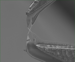
The present results were derived using the data previously reported by Fu et al. (Reference Fu, Fan and Hultmark2019) with the relevant parameters of the experimental conditions enumerated in table 1. The two velocity components were acquired simultaneously using a novel cross-wire probe with a measurement volume of  $42\ \mathrm {\mu } \text {m} \times 42\ \mu \text {m}\times 50\ \mathrm {\mu } \text {m}$. The two wires in the probe, shown in figure 1, were positioned orthogonal to each other and at
  $45^\circ$ relative to the pipe axis. The probe, dubbed the X-NSTAP, was based on the nanoscale thermal anemometry probe (NSTAP) design of Vallikivi & Smits (Reference Vallikivi and Smits2014) and Bailey et al. (Reference Bailey, Kunkel, Hultmark, Vallikivi, Hill, Meyer, Tsay, Arnold and Smits2010) used for measurements of longitudinal velocity. Here, two modified NSTAPs were fixed in close proximity with a
  $50\ \mathrm {\mu }\textrm {m}$ separation following the sandwiching procedure of Fan et al. (Reference Fan, Arwatz, Van Buren, Hoffman and Hultmark2015). The two wires were operated using separate channels of a Dantec Dynamics StreamLine Constant Temperature Anemometer circuit. The nominal overheat ratios were
  $R_w/R_0\approx 1.2$, where
  $R_w$ and
  $R_0$ represent the electrical resistances of the wires with and without Joule heating induced by the anemometry circuit, respectively. The resulting frequency response was estimated in still air using a square-wave test and found to exceed 150 kHz for each individual sensor. The velocity sensitivity of the probe was calibrated in situ using a Pitot tube (inner diameter of 0.89 mm). The static pressure at the streamwise location at the tip of the Pitot tube was measured using two pressure taps (0.40 mm diameter) located in the pipe wall. The local velocity at the Pitot tube was computed from the difference in pressure between the Pitot and static ports (Validyne DP15 transducers with 1379 Pa and 8618 Pa ranges). The angle sensitivity of the probe was determined with the stress-calibration method of Zhao, Li & Smits (Reference Zhao, Li and Smits2004) using at least 10 data points obtained in the core of the pipe. Corrections to the velocity calibration associated with the size of the Pitot tube diameter, turbulence intensity and velocity gradients outlined by McKeon et al. (Reference McKeon, Li, Jiang, Morrison and Smits2003) were applied but found to have a minimal effect on the data presented here. Measurements were acquired simultaneously from each wire at 300 kHz (National Instruments PCI-6123) and filtered using an analogue 8-pole Butterworth filter (Krohn-Hite Corporation) at 150 kHz. The acquisition period for each Reynolds number was at least
  $T_{samp} = 90\ \textrm {s}$, corresponding to
  $T_{samp} U_{cl}R^{-1} \geq 10 \times 10^3$ for all Reynolds numbers presented here.
Table 1. Experimental parameters for X-NSTAP measurements of turbulent pipe flow at high Reynolds numbers. Here,  $P_{abs}$ is the absolute pressure in the facility and
  $U_{cl}$ is the centreline velocity.


Figure 1. Scanning electron microscopy image of the X-NSTAP probe sensing elements. The two platinum sensing elements are shown perpendicular to each other to form an ‘X’. Each ribbon is  $60\ \mathrm {\mu }\textrm {m}$ long,
  $2\ \mathrm {\mu }\textrm {m}$ wide and
  $100$ nm thick. The wires are separated by a
  $50\ \mathrm {\mu }\textrm {m}$ thick spacer. The mean flow proceeds from left to right with the pipe radius aligned with the page vertical.
Measurements reported here were acquired at a radial location  $0.03R$ from the centreline, the closest location available in the data set. Radial gradients were approximated using statistics computed at the adjacent radial measurement location
  $0.05R$ from the centreline. The radial positioning of the probe was first determined with a depth microscope (Titan Tool Supply Inc., positioning accuracy of
  ${\pm }1 \ \mathrm {\mu }\textrm {m}$) and then tracked with a linear optical encoder (SENC50 Acu-Rite Inc., positioning accuracy of
  ${\pm }0.5\ \mathrm {\mu }\textrm {m}$). An electrical limit switch was also employed to ensure repeatable positioning of the probe between each test.
Importantly, the wire length in the sensor,  $\ell =60\ \mathrm {\mu }\textrm {m}$, is only slightly larger than twice the Kolmogorov length scale,
  $\eta = (\nu ^3/\epsilon _u)^{1/4}$, for the largest Reynolds number considered here. Following the procedure of Morrison et al. (Reference Morrison, Vallikivi and Smits2016) and Vallikivi (Reference Vallikivi2014), the errors in the spectral dissipation computed from (1.5a) and (1.5b) were estimated by assuming Kolmogorov scaling to be valid across all Reynolds numbers. Examining the deviations of the experimental spectra in Kolmogorov scaling, the errors were found to increase with
  $Re_\tau$ up to approximately
  $4\,\%$ for all but the highest Reynolds number examined here. The highest Reynolds number was found to have up
  $9\,\%$ error due to additional electrical noise in one of the signals during that acquisition. This level of attenuation is consistent with the 1 %–7 % error suggested by the exponential fit of Sadeghi, Lavoie & Pollard (Reference Sadeghi, Lavoie and Pollard2018) for a single component wire and the criteria outlined for a conventional X-wire by Wyngaard (Reference Wyngaard1968, Reference Wyngaard1969) to ensure less than
  $10\,\%$ error in both calculations of (1.5a) and (1.5b).
3. Results
3.1. Dimensionless dissipation estimates
The measurements of the current two-component data set were first validated against the corresponding single-component NSTAP measurements, showing excellent consistency with the analysis from Morrison et al. (Reference Morrison, Vallikivi and Smits2016). There, a Reynolds number dependence on the dimensionless dissipation rate,  $A=\epsilon R/ u_\tau ^3$, was calculated from the two different isotropic estimates of
  $\epsilon$ (namely (1.5a) and (1.8)) and shown in figure 2. While the data from Morrison et al. (Reference Morrison, Vallikivi and Smits2016) were restricted to just the longitudinal velocity component measurements obtained with an NSTAP, the present study obtained both longitudinal and transverse velocity measurements. In figure 2(a), the dissipation rate estimated from the integration of longitudinal spectra ((1.5a)) and transverse spectra ((1.5b)) were consistent with one another, indicating a measure of local isotropy at the small scales. In all cases, the transverse velocity estimate remained consistently higher, indicating that a small degree of error was likely introduced from the stress-calibration method. This discrepancy was largest for the two lower Reynolds number cases, up to
  $12\,\%$, likely due to increased thermal ‘cross-talk’ between the two wires associated with their close proximity. However, for
  $Re_\lambda > 200$, both estimates were within
  $5\,\%$ of each other and the single-component measurements of Morrison et al. (Reference Morrison, Vallikivi and Smits2016). Furthermore, the results of Morrison et al. (Reference Morrison, Vallikivi and Smits2016) demonstrated a behaviour consistent with the X-NSTAP results, giving an almost linear increase in
  $A$ with
  $Re_\lambda$. Similarly, the estimated dissipation from the K41 4/5 law followed an increasing trend and also agreed very well with Morrison et al. (Reference Morrison, Vallikivi and Smits2016). This underestimation from the 4/5 law was consistent with the recent findings of Antonia et al. (Reference Antonia, Tang, Djenidi and Zhou2019), in which it was found that over a range of experimental configurations and Reynolds numbers, the 4/5 law would not be achieved due to the influence of large scales and viscosity in the inertial range. Nonetheless, the longitudinal measurements from the present study, the NSTAP results of Morrison et al. (Reference Morrison, Vallikivi and Smits2016), and estimates from the transverse velocity were in good agreement.

Figure 2. Non-dimensional dissipation rate  $A=\epsilon R u_\tau ^{-3}$. Shown in (a) are:
  $\vartriangle$, the integration of longitudinal spectra (
 $\epsilon _u$) using (1.5a);
  $\triangledown$, the integration of transverse spectra (
 $\epsilon _v$) using (1.5b);
  $\square$, K41 4/5 law (
 $\epsilon _{\langle \Delta u^3 \rangle }$) given by (1.8). Filled symbols are results from the present data set and hollow/white symbols represent the corresponding parameter from Morrison et al. (Reference Morrison, Vallikivi and Smits2016). The hollow symbols are also repeated in (b) for reference. Shown in (b) are
  $\lhd$,
  $\epsilon _{\langle (\Delta u)^2 \rangle }$ using (1.14) and empirical coefficient
  $C_2=2$;
  $\rhd$,
  $\epsilon _{\langle (\Delta v)^2 \rangle }$ using (1.15) and empirical coefficient
  $C_2=2$;
  $\Diamond$, modified K41 4/5 law (
 $\epsilon _{C3}$) given by (1.16) to account for finite Reynolds number effects;
  $\circ$, generalized 4/5 law of Danaila et al. (Reference Danaila, Anselmet, Zhou and Antonia2001) using (1.10);
  $\times$, isotropic dissipation estimate from large scales (
 $\epsilon _{LS,iso}$) of Danaila et al. (Reference Danaila, Anselmet, Zhou and Antonia2001) given by (1.12);
  $+$, homogeneous dissipation estimate from large scales (
 $\epsilon _{LS,hom}$) of Danaila et al. (Reference Danaila, Anselmet, Zhou and Antonia2001) given by (1.13). Corresponding parameters in (b) from Morrison et al. (Reference Morrison, Vallikivi and Smits2016) were not reported.
These isotropic dissipation estimates were compared with several empirical estimates of dissipation, shown in figure 2(b). These estimates for  $A$ include the single-point approximations of Danaila et al. (Reference Danaila, Anselmet, Zhou and Antonia2001) for large-scale contributions ((1.12) and (1.13)), the empirical relations for the second-order structure functions ((1.14) and (1.15)), and modified third-order structure function ((1.16)). The empirical relations demonstrated remarkable consistency with one another, despite the relatively modest values of
  $Re_\lambda$. Conspicuously, these three empirical estimates fell between the values provided by the integrated spectrum and the third-order longitudinal structure functions. One potential explanation could be that each of these expressions utilizes an empirical coefficient, often argued as universal. If the ‘universal’ coefficient actually contains a dependency on Reynolds number, or if it is affected by the inhomogeneities and intermittency in the flow, then this would explain the discrepancy (see, for example, Antonia et al. Reference Antonia, Tang, Djenidi and Zhou2019). It could be argued that these estimates of
  $\epsilon$ from (1.14), (1.15) and (1.16) seemed to approach the estimates of the integrated spectra as
  $Re_\lambda$ increases, potentially indicating the lack of universality in the empirical constants, yet validating the need for higher
  $Re_\lambda$ to have truly inertial behaviour with local isotropy. This could additionally be argued by the lack of inertial range due to the limited
  $Re_\lambda$, resulting in an underestimate of
  $\epsilon$, and thus a lower value of
  $A$ predicted by the 4/5 law, while the second-order structure functions will more closely approach the actual dissipation for the same limited
  $Re_\lambda$. This was demonstrated in Antonia et al. (Reference Antonia, Tang, Djenidi and Zhou2019) where the empirical
  $C_2=2$ for the second-order structure functions was found to hold at lower Reynolds numbers compared to the requirement for the 4/5 law (cf. figure 7 in their paper).
For completeness, we included a dissipation estimate calculated from inertial range value using the generalized Kolmogorov formulation proposed by Danaila et al. (Reference Danaila, Anselmet, Zhou and Antonia2001) in (1.10) in figure 2(b). This refined analytic estimate surprisingly appears to agree well with the myriad of empirical estimates for dissipation derived from the second- and third-order structure functions, but still deviates from the more rigorous and common estimates plotted in figure 2(a). This lends further credence to the need for refining estimates of dissipation by including the contribution from non-homogeneous terms often neglected in the derivation of the popular estimates.
The behaviour of the above estimates differed noticeably from the large-scale dissipation estimate of Danaila et al. (Reference Danaila, Anselmet, Zhou and Antonia2001) in each case. For the isotropic large-scale estimate, corresponding to (1.12), the estimates were consistently 10 %–30 % larger than even the integrated spectra estimate for all but the lowest Reynolds number. However, the agreement was considerably improved for the homogeneous large-scale estimate from (1.13), which was within  $10\,\%$ of the integrated spectra estimate. The magnitude and trend of this behaviour was quantitatively similar to the experimental measurements presented by Danaila et al. (Reference Danaila, Anselmet, Zhou and Antonia2001) for a channel flow, however, no clear Reynolds number trend in these quantities was evident.
3.2. Second-order structure functions
Figure 3 shows both the second-order moments of the longitudinal and transverse velocity structure functions normalized according to (1.14) and (1.15) following K41 for each of the different Reynolds numbers. In contrast to Morrison et al. (Reference Morrison, Vallikivi and Smits2016) where the classic 4/5 law ((1.8)) was used to estimate the dissipation, here, both the longitudinal and transverse velocity structure functions are normalized with isotropic dissipation estimates determined from integrating their one-dimensional spectra,  $\epsilon _u$ and
  $\epsilon _v$, respectively. In each case, for separations
  $r<10\eta$, the behaviour of the structure functions is determined almost exclusively by viscous dissipation, consistent with the predictions of Kolmogorov (Reference Kolmogorov1941a). In the inertial range (e.g.
  $10 < r/\eta \leq 0.1 L/\eta$), where
  $L$ was the integral length scale, there was a clear growth in the peak value of both dimensionless second-order structure functions with Reynolds number approaching
  $2$ in the longitudinal case, and
  $8/3$ in the transverse case. Note the transverse data in figure 3 have been scaled by a constant to show both longitudinal and transverse components trending towards the same values. Kolmogorov (Reference Kolmogorov1941a) suggested that these constants are Reynolds number independent and high Reynolds number measurements would presumably yield a broader plateau approaching these values. Such behaviour is hinted at in the longitudinal case at the highest Reynolds number, while the transverse lags in the magnitude for the same Reynolds numbers. This again is consistent with the discussion from Chen et al. (Reference Chen, Sreenivasan, Nelkin and Cao1997) regarding the slower approach of the transverse velocity structure functions towards universality. In both cases, no definitive asymptotic value or plateau wider than a decade in the inertial range is observable in the current data set. Additionally, the growth with Reynolds number towards these values stands in contrast to the observations of Morrison et al. (Reference Morrison, Vallikivi and Smits2016), who observed a clear Reynolds number dependence in the peak value of the longitudinal structure function, but neither a monotonic trend nor plateau in the inertial range. Most of this discrepancy is perhaps due to the choice of the authors to normalize their structure functions with the dissipation estimate determined from the K41 4/5 law, in contrast with the integrated spectral estimate for
  $\epsilon _u$ and
  $\epsilon _v$ used here. Additionally, the peak values of the longitudinal and transverse structure function occur at different abscissae, which results in their ratio never approaching a constant.

Figure 3. Comparison of the normalized second-order structure functions: (coloured solid lines), longitudinal structure function of longitudinal velocity ( $\left \langle \Delta u^2\right \rangle /(\epsilon _u r)^{2/3}$); (coloured dashed lines), longitudinal structure function of transverse velocity (
 $3\left \langle \Delta v^2\right \rangle /(4(\epsilon _v r)^{2/3})$); (black solid line), small-scale dissipation estimate of longitudinal structure function (
 $\left \langle \Delta u^2\right \rangle =\epsilon _u r^2 /(15 \nu )$); (black thin dashed line), small-scale dissipation estimate of longitudinal structure function (
 $\left \langle \Delta v^2\right \rangle =\epsilon _v r^2 /(10 \nu )$); (black thin dotted line),
  $2$.
$2$.
In addition to the inertial range behaviour of the second-order structure functions, local isotropy constrains the relationship between the longitudinal and transverse velocity structure functions with (1.9). Figure 4 shows the ratio of the isotropic estimate of the transverse velocity structure function from (1.9) and the actual measured  $\left \langle (\Delta v)^2\right \rangle _{act}$ as a function of longitudinal separation,
  $r/\eta$. It is observed that at the pipe centreline, the isotropic estimate remains valid over two decades of separation
  $r/\eta$ for all Reynolds numbers in this study. This provides a clear indication that the assumption of local isotropy for the second-order structure functions holds along the pipe centreline, even at moderate Reynolds numbers.

Figure 4. Ratio of the isotropic estimate,  $\left \langle (\Delta v)^2\right \rangle _{iso}$ determined by (1.9) using
  $\left \langle (\Delta u)^2\right \rangle$, and the measured value for the second-order transverse velocity structure function at the pipe centreline.
3.3. One-dimensional wavenumber spectra
Shown in figures 5 and 6 are the normalized longitudinal and transverse spectral measurements in both their inner and outer scaling, given by the following equations:
 \begin{gather} f_1(k_x) = \phi_{uu}\epsilon_u^{{-}2/3}k_x^{5/3}, \end{gather}
 \begin{gather} g_1(k_x) = \phi_{vv}\epsilon_v^{{-}2/3}k_x^{5/3}. \end{gather}
Here, the streamwise wavenumber,  $k_x$, is obtained using Taylor's frozen field hypothesis with
  $k_x= {2{\rm \pi} f}/{U_{cl}}$, where
  $f$ is the spectral frequency. The longitudinal spectra of (3.1a) when plotted in both inner (viscous) and outer scaling (see figure 5) show behaviour that is consistent with Morrison et al. (Reference Morrison, Vallikivi and Smits2016), where no exact
  $5/3$ region was found. From the positive slope found in this compensated spectra, the observed slope in the inertial range is shallower than a
  $k_x^{-5/3}$ and closer to
  $k_x^{-1.6}$, consistent with Rosenberg et al. (Reference Rosenberg, Hultmark, Vallikivi, Bailey and Smits2013) and comparable to the empirical fit of Mydlarski & Warhaft (Reference Mydlarski and Warhaft1996) for the spectral exponent in grid turbulence (
 $-5/3 + 5.23 Re_\lambda ^{-2/3}$). Additionally, the spectral bump at
  $k_x\eta \approx 0.05$ was also present, as described by McKeon & Morrison (Reference McKeon and Morrison2007) and Morrison et al. (Reference Morrison, Vallikivi and Smits2016). Similar behaviour was observed in the transverse spectra in figure 6 where the slope in the inertial region remains shallower than the predicted
  $k_x^{-5/3}$. The behaviour in this region was further obscured by a more prominent spectral bump around
  $k_x\eta \approx 0.08$. Compensating the one-dimensional spectra for spatial intermittency according to Kolmogorov (Reference Kolmogorov1962) was also conducted similar to the analysis performed by Morrison et al. (Reference Morrison, Vallikivi and Smits2016). However, consistent with Morrison et al. (Reference Morrison, Vallikivi and Smits2016), this compensation did not improve the collapse in the longitudinal and transverse components and was therefore not included in this manuscript.

Figure 5. Compensated longitudinal wavenumber spectrum. (a) Kolmogorov scaling and (b) outer unit scaling. The vertical dashed lines indicate the approximate ordinate up to which spectral collapse is observed, namely (a)  $k_x \eta > 0.05$ and (b)
  $k_xR<5$.

Figure 6. Compensated transverse wavenumber spectrum. (a) Kolmogorov scaling and (b) outer unit scaling. The vertical dashed lines indicate the approximate ordinate up to which spectral collapse is observed, namely (a)  $k_x \eta > 0.1$ and (b)
  $k_xR<10$.
The ratio of the isotropic estimate of the transverse spectrum and the measured spectrum is shown in figure 7 in both inner and outer coordinates. In the low Reynolds number data, there is no evidence of an inertial range in the spectrum, with the ratio trending below 0.9 at high wavenumber. As  $Re_\lambda$ increases there is a discernible plateau spanning nearly a decade of an inertial range. However, similar to the lower Reynolds numbers, even the higher Reynolds numbers trend to slightly less than unity (0.9–0.95) for
  $k_x \eta >0.1$. This contrasts with figure 4, which showed slightly better agreement across a range of scales with the structure functions. The deviation towards the smaller scales from isotropic behaviour is due to the angle calibration leading to a slight error in the estimation of energy in each component. This is evidenced in figure 2(a), where
  $\epsilon _v$ slightly exceeds
  $\epsilon _u$. Additionally, the ratio of measured longitudinal and transverse spectra in figure 8 showed no inertial range for low
  $Re_\lambda$, but a growth with Reynolds number to nearly a decade of inertial range behaviour at
  $Re_\lambda = 411$. This behaviour agrees with Chamecki & Dias (Reference Chamecki and Dias2004), who found that a finite inertial range in the spectrum led to a smaller interval of inertial range in the structure functions.

Figure 7. Ratio of wall-normal spectra ( $\phi _{vv}$) and the isotropic estimate of
  $\phi _{vv}$ from the streamwise spectra given by K41 in (1.6). A value of unity implies isotropy at that the wavenumber. Inner scaling shown in (a), outer scaling in (b).

Figure 8. Ratio of wall-normal spectra ( $\phi _{vv}$) and the streamwise spectra (
 $\phi _{uu}$) given by (1.7). From Kolmogorov (Reference Kolmogorov1941a), the ratio between the spectra should be
  $4/3$ in the inertial region where we expect to see the
  $k_x^{-5/3}$ behaviour. Inner scaling shown in (a), outer scaling in (b).
3.4. Third-order structure functions
While the second-order structure functions demonstrated a trend toward inertial range behaviour as the Reynolds number increases, it was apparent that there was insufficient scale separation to elicit an inertial plateau. This can be seen in the third-order structure function  $\langle (\Delta u)^3 \rangle$ in figure 9, where none of the test cases exhibited a clear plateau at the centreline for all ranges of
  $r/\eta$ and the peak values fall well short of the 4/5 law.

Figure 9. Third-order structure functions  $\langle (\Delta u)^3\rangle$ and the terms from (1.10): (coloured solid lines), the inertial contribution, Term I; (small coloured dashed lines), the viscous contribution, Term II; (coloured dashed lines), the non-homogeneous component, Term III. The sum of the three terms is given by the thicker, darker lines. The constant
  $4/5$ is shown by the thin dashed line.
Growth in the value of the structure function was consistent with the observations of Antonia et al. (Reference Antonia, Tang, Djenidi and Zhou2019). Comparison of Term I in figure 9 to Antonia et al. (Reference Antonia, Tang, Djenidi and Zhou2019) (cf. their figure 3a) showed the predicted behaviour of the 4/5 law matching the cases shown in this study. These results stand in contrast to the comparable results of Morrison et al. (Reference Morrison, Vallikivi and Smits2016) where all normalized third-order moments of the structure function followed a similar curve, approaching a peak value of 0.6–0.7 at  $r\eta ^{-1} \approx 40$. Again, some of this discrepancy is likely due to the authors’ choice of normalizing the moments by a dissipation estimate derived from the structure functions. This current study normalizes the third-order moments with the spectral dissipation estimate given by
  $\epsilon _u$ and exhibits excellent collapse in the viscous range and a clear growth in the peak value with increasing Reynolds number. Additionally, the dimensionless third-order moments remain non-zero over an increasingly wide range of
  $r/\eta$ with increasing Reynolds number.
Improvements to the third-order structure function behaviour are found through including the neglected corrections over the range of scales which were unavailable in the data used by Morrison et al. (Reference Morrison, Vallikivi and Smits2016). Shown in figure 9 are the additional terms of the generalized 4/5 law of Danaila et al. (Reference Danaila, Anselmet, Zhou and Antonia2001) from (1.10). Term I is the original 4/5 law, Term II is the viscous contribution, which dominates the small scales, and Term III is the influence of inhomogeneity within the flow, which comes to dominate the large scales as  $r$ increases. Note that Term IV from (1.11) is not included due to the analysis taking place near the centreline, and calculations at all Reynolds numbers found it to be negligible across all scales. The sum of these three terms should add to 4/5 and is also shown in figure 9. By choosing
  $\epsilon _u$ as the dissipation scale, the agreement between the different Reynolds numbers through the inclusion of the non-homogeneous term was evident. With the exception of the lowest Reynolds number, each of the curves collapses to a value
  $\approx 0.7$. As the separation
  $r$ increases, the non-homogeneous term dominates and exceeds 0.8 for the two lowest Reynolds numbers. These large values likely stem from a combination of lower statistical convergence of the non-homogenous term at larger values of
  $r$ amplified by the small radial separation of the measurement points used to compute the gradients.
Similar to the expanded 4/5 law, Danaila et al. (Reference Danaila, Anselmet, Zhou and Antonia2001) developed a generalized expression for the third-order structure functions
 \begin{equation} \underbrace{-\frac{\left\langle(\Delta u)(\Delta u_i)^2\right\rangle}{\epsilon r}}_{\text{Term I}} + \underbrace{\frac{2\nu}{\epsilon r} \frac{\mathrm{d}}{\mathrm{d} r}\left\langle(\Delta u_i)^2\right\rangle}_{\text{Term II}} + \underbrace{\frac{2}{\epsilon r^3}\int_0^r s^2\left(-\frac{\partial (v(\Delta u_i)^2)}{\partial y}\right) \mathrm{d}s}_{\text{Term III}} = \frac{4}{3}. \end{equation}
Equation (3.2) provides additional insight into the behaviour of the flow, as it has not fully utilized the isotropic relations to simplify the summation over  $i$. Figure 10 shows the terms of (3.2), with Term I representing the third-order structure functions, Term II representing the viscous contribution and Term III representing the large-scale inhomogeneities. The sum of the three terms is also shown. As was the case with figure 9, the third-order terms did not reach a plateau of 4/3 alone, but did exhibit a trend towards the plateau with increasing
  $Re_\lambda$. Inclusion of the viscous and non-homogeneous terms improved the estimate, but good agreement was not found, contrary to the case in figure 9. For all Reynolds numbers, it appeared that the generalized expression was not as close to 4/3 over the range of separation
  $r$ compared with how well the longitudinal terms added to
  $4/5$ in figure 9. However, the sum more closely approaches 4/3 for wider ranges of
  $r\eta ^{-1}$ with increasing Reynolds number.

Figure 10. Generalized expression for the third-order structure functions given by (3.2): (coloured solid lines), the inertial contribution, Term I; (small coloured dashed lines), the viscous contribution, Term II; (coloured dashed lines), the non-homogeneous component, Term III. The sum of the three terms is given by the thicker, darker lines, and the constant  $4/3$ is shown as a thin dashed black line.
The rate of convergence towards an inertial range can be seen in figure 11, which plots the peak values of the longitudinal and mixed structure functions. They are compared to the empirical coefficient  $C_3$ of Lundgren (Reference Lundgren2002), which describes the rate of convergence towards inertial range behaviour of the longitudinal structure functions. This coefficient was found for the tangent line to their matched asymptotic expansion of the 4/5 law. The data for
  $\left \langle (\Delta u)^3\right \rangle$ exhibit a slower approach to
  $4/5$ than the
  $C_3$ curve, with a dependence closer to
  $Re_\lambda ^{-0.46}$. Although these measurements comparatively exceed those for
  $\left \langle (\Delta u)(\Delta u_i)^2\right \rangle$ in their approach to inertial range behaviour at each Reynolds number, the measurements of
  $\left \langle (\Delta u)(\Delta u_i)^2\right \rangle$ exhibit a similar Reynolds number dependence following
  $Re_\lambda ^{-0.52}$.

Figure 11. Approach to inertial range behaviour for the 4/5 and 4/3 laws. All values are normalized to approach unity. The relationship of Lundgren (Reference Lundgren2002) for decaying isotropic turbulence is represented by the solid blue line corresponding to  $C_3 = 0.8-8.45 Re_\lambda ^{-2/3}$ from (1.16). Circles represent the maximum value of
  $\left \langle (\Delta u)^3\right \rangle$ in this study with a power law fit following the blue dashed line given by
  $C_3 = 0.8-3.712Re_\lambda ^{-0.46}$. Squares represent the maximum values of
  $\left \langle (\Delta u)(\Delta u_i)^2\right \rangle$ and a power law fit following the red dashed line given by
  $C_3 = 1.33- 10.55Re_\lambda ^{-0.52}$.
4. Discussion
In estimating the dissipation through isotropic relations, figure 2(a) clearly indicates that measurements of both longitudinal and transverse velocity are largely matching and corroborating the findings of Morrison et al. (Reference Morrison, Vallikivi and Smits2016). It also demonstrates that the 4/5 law in its classical form under-predicts dissipation, as expected. This is consistent with the analysis by Chamecki & Dias (Reference Chamecki and Dias2004), who found a lack of validity in the third-order isotropic relations over their range of cases ( $6800< Re_\lambda <14\,000$) and an underprediction of the dissipation rate compared with the spectral estimates. The current results shown in figure 2(a) demonstrate a similar discrepancy, but figure 2(b) shows how the modified equation from Danaila et al. (Reference Danaila, Anselmet, Zhou and Antonia2001) reduces this discrepancy from the 4/5 law estimate. Additionally, the modified 4/5 law results in the dissipation calculations closely matching the empirical expressions of Lundgren (Reference Lundgren2002) and Chamecki & Dias (Reference Chamecki and Dias2004). While it is apparent that this modified 4/5 law still does not match the spectral estimate, accounting for the large-scale inhomogeneities improves the estimate considerably. This discrepancy indicates the assumption of a fully inertial range is not appropriate for the Reynolds numbers studied here, and could be due to terms neglected in the isotropic assumptions in deriving (1.10) that become relevant at these lower Reynolds numbers. The continued influence of outer boundary conditions is indicated by the increasing value of
  $A$ in figure 2, consistent with Morrison et al. (Reference Morrison, Vallikivi and Smits2016). While
  $A$ is claimed to be a constant in the inertial range, the present results align with previous findings which show that an inertial range is not present until
  $Re_\lambda > 1000$, or even
  $2000$ in shear flow cases (Saddoughi & Veeravalli Reference Saddoughi and Veeravalli1994; Saddoughi Reference Saddoughi1997; Antonia & Burattini Reference Antonia and Burattini2006).
The behaviour of the second-order structure functions also indicates that the small scales are isotropic while the inertial behaviour is continuing to evolve. Figure 3 clearly shows classical dissipative range behaviour where the structure functions match the Kolmogorov (Reference Kolmogorov1941a) isotropic estimate for  $r<10\eta$ in both longitudinal and transverse velocities. Figure 4 further shows how the isotropic estimate of the second-order transverse structure function closely matches the actual measurement. However, at larger separations, the peak value of the second-order structure functions continues to grow as Reynolds number increases, indicating that the inertial range behaviour is not yet universal. This is further evident by the lack of a
  $-5/3$ region in both the longitudinal and transverse spectra, consistent with Morrison et al. (Reference Morrison, Vallikivi and Smits2016) for their longitudinal measurements. The consistency across components is yet another indication that, while isotropy of the small scales is holding for the dissipation estimates, fully inertial behaviour has not been obtained.
These results from the spectral data and second-order structure functions emphasize the need for utilizing the modified 4/5 law approach of Danaila et al. (Reference Danaila, Anselmet, Zhou and Antonia2001) for a correct interpretation of the third-order structure functions. Comparing figures 9 and 10 provides clear evidence of improved behaviour and wider ranging validity of the 4/5 and 4/3 laws when including viscous and non-homogeneous contributions. The modified 4/5 law developed by Danaila et al. (Reference Danaila, Anselmet, Zhou and Antonia2001) results in a larger range of  $r\eta ^{-1}$ for which the third-order longitudinal moment approaches a plateau, and the overall accuracy considerably improves for increasing
  $Re_\lambda$, with the highest Reynolds number case nearly matching 4/5 for the entire range of scales. The errors at these large separations are decreasing for increasing
  $Re_\lambda$, both due to the increase in independent samples and the approach towards inertial range behaviour.
A better understanding of this need for correction can be found from the results of the generalized  $4/3$ equation, which shows a further deviation from the constant value compared with the
  $4/5$ equation. It was demonstrated by Shen & Warhaft (Reference Shen and Warhaft2000) that significant anisotropy exists in the higher-order odd moments, even while the second-order moments have the predicted isotropic behaviour. This holds consistent with second-order moments shown in figure 3, and indicates that the transverse components are clearly not contributing sufficiently towards the 4/3 law as would be assumed under local isotropy. This results in the sum of the terms of (3.2) not matching
  $4/3$ as closely, but the consistent trend of increased accuracy for larger
  $Re_\lambda$ is present. Further evidence that accounting for inhomogeneities and anisotropic contributions at these lower Reynolds numbers is necessary can be drawn from the study of Chen et al. (Reference Chen, Sreenivasan, Nelkin and Cao1997), who found that the longitudinal and transverse velocity increments cannot behave the same, as the transverse increment
  $\Delta v$ has a larger flatness value over all ranges of separation
  $r$, indicating a greater intermittency. Therefore, these higher-ordered mixed structure functions will have a slower approach towards their inertial range behaviour, consistent with our results. Higher values of
  $Re_\lambda$ must be achieved to obtain accurate estimates of the 4/3 law vs the 4/5 law.
Comparing figure 10 with the results of Burattini, Antonia & Danaila (Reference Burattini, Antonia and Danaila2005), who analysed a version of the modified 4/3 law in a turbulent round jet at  $Re_\lambda = 363$, shows our results under-predicting the 4/3 value compared with theirs. The range of
  $r\eta ^{-1}$ with the greatest deviation from Burattini et al. (Reference Burattini, Antonia and Danaila2005) corresponds to the location of non-homogeneous contributions, including a production term not present in (3.2). However, general trends in the behaviour of comparable terms are in agreement across the studies. The non-homogeneous component is found to be dominant for larger separations, and a comparison of our case to
  $Re_\lambda =361$ shows that the separation of
  $r\eta ^{-1}>100$ (corresponding to
  $r\lambda ^{-1}>3$) is comparable to their conclusion on the dominance of the non-homogeneous contribution in a round jet. In addition to the transverse third-order structure functions not sufficiently contributing to the balance, deviation from the modified 4/3 law could be due to the omission of components neglected in the derivation of (3.2) (and likewise (1.10) for the 4/5 law). The assumption of isotropy inherently neglects the pressure correlation terms, and although they cannot be measured in this experimental set-up, it is possible they account for some of the deviations at these lower Reynolds numbers (see Sadeghi et al. Reference Sadeghi, Lavoie and Pollard2018). Additionally, there are derivative terms that become negligible with local homogeneity that may need to be retained in the derivation for these lower Reynolds numbers (see Danaila et al. Reference Danaila, Anselmet, Zhou and Antonia2001). Nonetheless, the trend shows an approach to 4/3 and decreasing influence of the non-homogeneous component with increasing
  $Re_\lambda$.
The approach toward an inertial range as depicted in figure 11 provides a summary of all of the previous discussion. It is apparent that the peak of the 4/5 law (and corresponding 4/3 law) grows with Reynolds number, and the behaviour in the pipe indicates a slower growth than the theoretical analysis of Lundgren (Reference Lundgren2002), which did not include mean shear in the flow. Their work utilized matched asymptotics to derive a composite expansion for  $\left \langle (\Delta u)^3\right \rangle$, and the empirical fit of the tangent line to their expression gave the rate at which the 4/5 law is approached. This asymptotic expansion was for the Kármán–Howarth equation (von Kármán & Howarth Reference von Kármán and Howarth1938) and therefore did not account for any large scale inhomogeneities. The slower approach of
  $\left \langle (\Delta u)^3\right \rangle$ from the pipe flow therefore conforms with expectations that shear flow and anisotropy will lead to deviations from the 4/5 law (Hill Reference Hill1997; Chamecki & Dias Reference Chamecki and Dias2004). While the deviation of the mixed structure functions from the 4/3 law was found to be larger at the same Reynolds numbers than those in the 4/5 law, the power on the
  $Re_\lambda$ dependence indicates a similar rate of approach. However, the limited range of data prevents any significant insight being drawn on these fit exponents.
5. Conclusions
We have applied the generalized 4/5 and 4/3 laws near the centreline of turbulent pipe flow and found that accounting for inhomogeneities provides significant improvement to the approach towards 4/5 (and 4/3), consistent with Danaila et al. (Reference Danaila, Anselmet, Zhou and Antonia2001). This study adds pipe flow to the body of flow configurations in which the generalized approach has been successfully applied, including a wide range of flow configurations such as channels (Danaila et al. Reference Danaila, Anselmet, Zhou and Antonia2001), decaying turbulence (Antonia & Burattini Reference Antonia and Burattini2006) and jets (Burattini et al. Reference Burattini, Antonia and Danaila2005; Sadeghi et al. Reference Sadeghi, Lavoie and Pollard2018).
By using a combination of a high pressure facility and nanoscale, two-component hot-wires, we were able to probe the behaviour of the inertial subrange and local isotropy assumption near the centreline of turbulent pipe flow up to  $Re_\lambda = 411$. Measurements of multiple velocity components with wire lengths only slightly larger than twice the Kolmogorov length scale facilitated the evaluation of the local isotropy assumption as well as the influence of inhomogeneities in the generalized Kolmogorov balance with minimal effects from spatial filtering. The derivation of the generalized equation in a pipe flow results in (1.11), which simplifies along the pipe centreline to the expression of Danaila et al. (Reference Danaila, Anselmet, Zhou and Antonia2001), allowing use of (1.10). Although local isotropy cannot be evaluated entirely, as that task requires the complete strain-rate tensor, the majority of isotropic flow relations evaluated in this study were found to be satisfied for second-order statistics. This study complements the results of Morrison et al. (Reference Morrison, Vallikivi and Smits2016) by adding measurements of an additional velocity component due to the use of the X-NSTAP. Importantly, the new transverse measurements show similar behaviour that results in a constant increase in the supposed universal value of the factor
  $A$, when scaled with
  $u_\tau$ and
  $R$. Additionally, the K41 estimate for dissipation tracks their estimate, corroborating this constant increase in
  $A$. Comparing these results to the generalized expression of Danaila et al. (Reference Danaila, Anselmet, Zhou and Antonia2001) and empirical estimates of dissipation shows consistency between each calculation, and also demonstrates an improvement on the K41 estimate alone. However, these inertial range estimates do not obtain the same value of
  $A$ that both isotropic spectral measurements give.
The analysis of Danaila et al. (Reference Danaila, Anselmet, Zhou and Antonia2001) was extended to the pipe geometry, where we found consistency with their derived budget and results. The additional pseudo-production term derived in the pipe geometry is negligible near the centreline, allowing the use of the generalized 4/5 equation of Danaila et al. (Reference Danaila, Anselmet, Zhou and Antonia2001). Further analysis indicates a lack of local isotropy in the third-order structure functions. Contributions from the non-homogeneous terms are found to be necessary when considering the energy budget near the centreline. However, even accounting for these effects does not yield a  $4/5$ or
  $4/3$ range within the inertial range at the Reynolds numbers in this study. The generalized
  $4/5$ equation has better behaviour over the range of separations compared to the generalized
  $4/3$ equation, indicating that the assumptions applied in deriving these equations may not hold. This could be due to inhomogeneities stemming from the mean shear in pipe flow preventing local isotropy from being attained in the third-order structure functions until significantly higher Reynolds numbers (Hill Reference Hill1997), unlike decaying isotropic turbulence behind a grid. Additionally, the intermittency of the transverse component could prevent isotropic behaviour until significantly higher Reynolds numbers. Another breakdown in the assumptions behind (1.10) would be if the pressure–velocity correlations are non-zero, which would account for a contribution that cannot be evaluated in this current data set. This potential effect was discussed by Sadeghi et al. (Reference Sadeghi, Lavoie and Pollard2018) in their extended budget in a round jet, where additional production and diffusion terms were accounted for off centreline but deviations from the predicted sum still persisted. Lastly, the rate at which the 4/5 and 4/3 laws were approached by the third-order structure functions was evaluated and found to be more gradual than decaying isotropic turbulence for the same Reynolds numbers. In each case, the approach to the predicted asymptotic decayed approximately as
  $Re_\lambda ^{-0.5}$ in contrast to the decaying grid turbulence (
 $Re_\lambda ^{-2/3}$) or forced turbulence (
 $Re_\lambda ^{-5/6}$) (Antonia & Burattini Reference Antonia and Burattini2006). A potential measure to provide more accurate dissipation measurements through higher-order statistics could be performed by estimating the dissipation through axisymmetric relations (see Anselmet, Antonia & Ould-Rouis Reference Anselmet, Antonia and Ould-Rouis2000), but the current X-NSTAP measurements are not able to extract the fourth velocity derivative needed. Establishing an extensive inertial range in the 4/5 and 4/3 laws requires higher Reynolds number investigations which are achievable in the Princeton Superpipe. However, more specialized probes and measurement techniques are required to achieve the necessary small-scale resolution.
Acknowledgements
The authors would like to thank Y. Fan for his aid in fabricating the probes and acquiring the data using in this study and K. Huang for her help in editing the paper.
Funding
This work was supported by under NSF grant CBET-1510100 (program manager R. Joslin) and the Office of Naval Research (ONR) grant N00014-17-2309.
Declaration of interests
The authors report no conflict of interest.
Appendix A. Generalized Kolmogorov equation for centreline pipe flow
To derive (1.11), the process outlined in Danaila et al. (Reference Danaila, Anselmet, Zhou and Antonia2001) or Burattini et al. (Reference Burattini, Antonia and Danaila2005) will be used. Starting with the incompressible Navier–Stokes equations at two different longitudinal points, denoted by  $x$ and
  $x^+$, decomposing the velocities and pressures into a mean plus a fluctuation and assuming the mean at both points is the same based on the idea of longitudinal homogeneity and small changes off the centreline of the pipe, then subtracting the two equations from each other results in
 $$\begin{gather} \frac{\partial}{\partial t}\left(\Delta u_i\right) + \Delta\left(U_j\frac{\partial u_i}{\partial x_j}\right)+ \Delta\left(u_j\frac{\partial U_i}{\partial x_j}\right)+ u_j^+\frac{\partial^+}{\partial x_j}\left(\Delta u_i\right) + u_j\frac{\partial}{\partial x_j}\left(\Delta u_i\right) \nonumber\\ ={-}\left(\frac{\partial}{\partial x_i} +\frac{\partial^+}{\partial x_i}\right)\frac{\Delta p}{\rho} + \nu\left(\frac{\partial^2}{\partial x_j^2} +\frac{\partial^{2^+}}{\partial x_j^2}\right)\left(\Delta u_i\right), \end{gather}$$
where  $U_i$ is the mean velocity in the
  $i$ direction,
  $u_i$ is the velocity fluctuation in the
  $i$ direction and the velocity increment is denoted as
  $\Delta u_i = u_i(\boldsymbol {x}^+)-u_i(\boldsymbol {x})$. The fourth and fifth terms on the left-hand side of (A1) are a result of the independence of
  $u_i$ from
  $x_j^+$ and
  $u_i^+$ from
  $x_j$. Next, add and subtract the term
  $u_j({\partial ^+}/{\partial x_j})(\Delta u_i)$ to the left-hand side of (A1) and combine terms to get
 $$\begin{gather} \frac{\partial}{\partial t}\left(\Delta u_i\right) + \Delta\left(U_j\frac{\partial u_i}{\partial x_j}\right)+ \Delta\left(u_j\frac{\partial U_i}{\partial x_j}\right)+ \left(\Delta u_j\right) \frac{\partial^+}{\partial x_j}\left(\Delta u_i\right) + u_j\left[\frac{\partial^+}{\partial x_j} + \frac{\partial}{\partial x_j}\right]\left(\Delta u_i\right) \nonumber\\ ={-}\left(\frac{\partial}{\partial x_i}+\frac{\partial^+}{\partial x_i}\right)\frac{\Delta p}{\rho} + \nu\left(\frac{\partial^2}{\partial x_j^2} +\frac{\partial^{2^+}}{\partial x_j^2}\right)\left(\Delta u_i\right). \end{gather}$$
Next, multiply (A2) by  $\Delta u_k$ and treat it in the same way the Reynolds stress equation is derived by taking a copy of that expression, swapping the indices
  $i$ and
  $k$, then adding them together, which allows the combination of most every term due to the fact that they are expanded product rules of derivatives
 $$\begin{gather} \frac{\partial}{\partial t}\left(\Delta u_i\Delta u_k\right) + \left(\Delta u_k\right) \Delta\left(U_j\frac{\partial u_i}{\partial x_j}\right)+ \left(\Delta u_i\right) \Delta\left(U_j\frac{\partial u_k}{\partial x_j}\right)+ \left(\Delta u_k\right) \Delta\left(u_j\frac{\partial U_i}{\partial x_j}\right) \nonumber\\ + \left(\Delta u_i\right) \Delta\left(u_j\frac{\partial U_k}{\partial x_j}\right) + \left(\Delta u_j\right) \frac{\partial^+}{\partial x_j}\left(\Delta u_i\Delta u_k\right) + u_j\left[\frac{\partial^+}{\partial x_j} + \frac{\partial}{\partial x_j}\right]\left(\Delta u_i\Delta u_k\right) \nonumber\\ ={-}\left(\Delta u_k\right) \left(\frac{\partial}{\partial x_i}+\frac{\partial^+}{\partial x_i}\right)\frac{\Delta p}{\rho} -\left(\Delta u_i\right) \left(\frac{\partial}{\partial x_k}+\frac{\partial^+}{\partial x_k}\right)\frac{\Delta p}{\rho}\nonumber\\ + \nu \Delta u_k\left(\frac{\partial^2}{\partial x_j^2} +\frac{\partial^{2^+}}{\partial x_j^2}\right)\left(\Delta u_i\right) + \nu \Delta u_i \left(\frac{\partial^2}{\partial x_j^2} +\frac{\partial^{2^+}}{\partial x_j^2}\right)\left(\Delta u_k\right) . \end{gather}$$
This expression can be significantly simplified by applying a few assumptions. Equation (A3) is ensemble averaged, statistical stationarity and local isotropy are assumed, and the continuity equation allows terms 6 and 7 on the left-hand side to have their velocity increments to be brought into the derivatives. Therefore, (A3) is now
 $$\begin{gather} \left\langle\left(\Delta u_k\right) \Delta\left(U_j\frac{\partial u_i}{\partial x_j}\right)\right\rangle+ \left\langle\left(\Delta u_i\right) \Delta\left(U_j\frac{\partial u_k}{\partial x_j}\right)\right\rangle+ \left\langle\left(\Delta u_k\right) \Delta\left(u_j\frac{\partial U_i}{\partial x_j}\right)\right\rangle \nonumber\\ + \left\langle\left(\Delta u_i\right) \Delta\left(u_j\frac{\partial U_k}{\partial x_j}\right)\right\rangle + \frac{\partial^+}{\partial x_j}\left\langle\Delta u_j\Delta u_i\Delta u_k\right\rangle + \left[\frac{\partial^+}{\partial x_j} + \frac{\partial}{\partial x_j}\right]\left\langle u_j\Delta u_i\Delta u_k\right\rangle\nonumber\\ = \nu \left\langle\Delta u_k\left(\frac{\partial^2}{\partial x_j^2} +\frac{\partial^{2^+}}{\partial x_j^2}\right)\left(\Delta u_i\right)\right\rangle + \nu \left\langle\Delta u_i \left(\frac{\partial^2}{\partial x_j^2} +\frac{\partial^{2^+}}{\partial x_j^2}\right)\left(\Delta u_k\right)\right\rangle. \end{gather}$$
Under the assumption of local homogeneity (see Hill Reference Hill1997) spatial derivatives are written with respect to the separation between points. It can be shown that
 \begin{equation} \frac{\partial}{\partial x_k} ={-}\frac{\partial}{\partial r_k} ;\quad \frac{\partial}{\partial x_k^+} = \frac{\partial}{\partial r_k}, \end{equation}
which allows (A4) to be written as
 $$\begin{gather} \left\langle\left(\Delta u_k\right) \Delta\left(U_j\frac{\partial u_i}{\partial x_j}\right)\right\rangle+ \left\langle\left(\Delta u_i\right) \Delta\left(U_j\frac{\partial u_k}{\partial x_j}\right)\right\rangle+ \left\langle\left(\Delta u_k\right) \Delta\left(u_j\frac{\partial U_i}{\partial x_j}\right)\right\rangle\nonumber\\ + \left\langle\left(\Delta u_i\right) \Delta\left(u_j\frac{\partial U_k}{\partial x_j}\right)\right\rangle + \frac{\partial}{\partial r_j}\left\langle\Delta u_j\Delta u_i\Delta u_k\right\rangle + \left[\frac{\partial^+}{\partial x_j} + \frac{\partial}{\partial x_j}\right]\left\langle u_j\Delta u_i\Delta u_k\right\rangle\nonumber\\ = 2\nu \frac{\partial^2}{\partial r^2_j}\left\langle\Delta u_i\Delta u_k\right\rangle - \frac{4}{3}\epsilon\delta_{i,k}. \end{gather}$$
Note that the viscous terms on the right-hand side of (A6) are a result of local homogeneity and isotropy to obtain the expression for dissipation. Also note that, with the exception of the fifth term on the left-hand side of this equation, the remaining derivatives are not transformed into derivatives with respect to separation. This is due to these terms being a result of large-scale inhomogeneities.
Up to this point, the math and process is similar to the initial steps taken in Danaila et al. (Reference Danaila, Anselmet, Zhou and Antonia2001) for the channel flow or Burattini et al. (Reference Burattini, Antonia and Danaila2005) for the jet. The remainder of the derivation follows their steps but has an additional large-scale inhomogeneous term as a result of the pipe flow geometry. It is to these large-scale inhomogeneities that the remainder of this derivation will focus on. Terms 1 and 2 on the left-hand side of (A6) can be combined, resulting in:
 \begin{equation} \left\langle\left(\Delta u_k\right) \Delta\left(U_j\frac{\partial u_i}{\partial x_j}\right)\right\rangle\!+ \left\langle\left(\Delta u_i\right) \Delta\left(U_j\frac{\partial u_k}{\partial x_j}\right)\right\rangle \!=\! \left\langle U_j^+\frac{\partial^+ }{\partial x_j}\left(\Delta u_k \Delta u_i\right)\right\rangle - \left\langle U_j\frac{\partial}{\partial x_j}\left(\Delta u_k \Delta u_i\right)\right\rangle\!. \end{equation}
For the system of a fully developed turbulent pipe, longitudinal homogeneity, azimuthal homogeneity and zero axial velocity require
 \begin{equation} U_x\frac{\partial}{\partial x} = \frac{U_\theta}{r}\frac{\partial}{\partial \theta} = U_r\frac{\partial}{\partial r} = 0. \end{equation}
Therefore, in this system, the two terms on the right-hand side of (A7) are identically zero in all points in the flow.
The exact same process of expanding terms is applied to terms 3 and 4 on the left-hand side of (A6), where we can see the following:
 \begin{equation} \left\langle\left(\Delta u_k\right) \Delta\left(u_j\frac{\partial U_i}{\partial x_j}\right)\right\rangle + \left\langle\left(\Delta u_i\right) \Delta\left(u_j\frac{\partial U_k}{\partial x_j}\right)\right\rangle =\left\langle\Delta u_k \Delta u_j\right\rangle \frac{\partial U_i}{\partial x_j} +\left\langle\Delta u_i \Delta u_j\right\rangle \frac{\partial U_k}{\partial x_j}. \end{equation}
In a fully developed pipe flow, if the displacements between  $x_j$ and
  $x_j^+$ are simply in the longitudinal direction, which is often the direction of separation in the evaluation of structure functions, the mean gradient is therefore a constant. Furthermore, in the fully developed pipe, the only mean shear that exists is the longitudinal velocity in the radial direction, which means the terms in (A9) that are not
  $j=2$ or
  $i=k=1$ terms are identically zero
 \begin{equation} \left\langle\Delta u_k \Delta u_j\right\rangle \frac{\partial U_i}{\partial x_j} +\left\langle\Delta u_i \Delta u_j\right\rangle \frac{\partial U_k}{\partial x_j} = 2\left\langle\Delta u \Delta v\right\rangle \frac{d U}{\textrm{d} y}. \end{equation}
Additionally, recognizing that the sixth term on the left-hand side of (A6) must be applied with the separation between  $x_j$ and
  $x_j^+$ occurring in the longitudinal direction allows them to combine due to longitudinal homogeneity. Therefore, plugging (A10) into (A6) will result in
 \begin{equation} 2\left\langle\Delta u \Delta v\right\rangle \frac{d U}{\textrm{d} y} + \frac{\partial}{\partial r_j}\left\langle\Delta u_j\Delta u_i\Delta u_k\right\rangle + 2\frac{\partial}{\partial x_j}\left\langle u_j\Delta u_i\Delta u_k\right\rangle = 2\nu \frac{\partial^2}{\partial r^2_j}\left\langle\Delta u_i\Delta u_k\right\rangle - \frac{4}{3}\epsilon \delta_{i,k}. \end{equation}
Both term 2 on the left-hand side and term 1 on the right-hand side of (A11) can be simplified significantly through the use of isotropic relations. As laid out in chapters 13 and 22 of Monin & Yaglom (Reference Monin and Yaglom2013), these two terms can each be expressed as a single scalar function. Projecting the separation along the longitudinal direction and summing over matched indices, the following expression can be found for the second-order structure function:
 $$\begin{gather} 2\nu \frac{\partial^2}{\partial r^2_j}\left\langle\Delta u_i\Delta u_k\right\rangle = 10\nu \frac{\textrm{d}^2}{\textrm{d} r^2}\left\langle\left(\Delta u\right)^2\right\rangle + 2\nu r\frac{\textrm{d}^3}{\textrm{d} r^3}\left\langle\left(\Delta u\right)^2\right\rangle\nonumber\\ =\frac{2\nu}{r^4}\frac{\textrm{d}}{\textrm{d}r}\left(r^5\frac{\textrm{d}^2}{\textrm{d}r^2}\left\langle\left(\Delta u\right)^2\right\rangle\right), \end{gather}$$
and for the third-order structure function
 $$\begin{gather} \frac{\partial}{\partial r_j}\left\langle\Delta u_j\Delta u_i\Delta u_k\right\rangle =\frac{5}{3}\frac{\textrm{d}}{\textrm{d} r}\left\langle\left(\Delta u\right)^3\right\rangle + \frac{r}{3}\frac{\textrm{d}^2}{\textrm{d} r^2}\left\langle\left(\Delta u\right)^3\right\rangle\nonumber\\ = \frac{1}{3r^4} \frac{\textrm{d}}{\textrm{d}r}\left(r^5 \frac{\textrm{d}}{\textrm{d}r}\left\langle\left(\Delta u\right)^3\right\rangle\right). \end{gather}$$
Note that the indices have ended up becoming restricted to  $i=k=1$ in the assumption of the longitudinal direction of separation and application of isotropic tensors.
Treatment of term three of (A11), or the second non-homogeneous term, follows the arguments of Danaila et al. (Reference Danaila, Anselmet, Zhou and Antonia2001) in which they assumed then demonstrated the non-homogeneous term behaves in a similar manner to the second-order structure function (cf. (2.10)–(2.12) of Danaila et al. Reference Danaila, Anselmet, Zhou and Antonia2001). That allows the following simplification:
 $$\begin{gather} 2\frac{\partial}{\partial y}\left\langle v \Delta u_i\Delta u_i\right\rangle =2\left[ 3\frac{\partial}{\partial y}\left\langle v \left(\Delta u\right)^2\right\rangle + r\frac{\textrm{d}}{\textrm{d} r}\frac{\partial}{\partial y}\left\langle v \left(\Delta u\right)^2\right\rangle\right]\nonumber\\ = \frac{2}{r^2}\frac{\textrm{d}}{\textrm{d} r}\left(r^3 \frac{\partial}{\partial y} \left\langle v\left(\Delta u\right)^2\right\rangle\right), \end{gather}$$
since longitudinal homogeneity and axial symmetry mean there are no  $x$ or
  $z$ derivatives of mean quantities. Note that the separation
  $r$ is in the longitudinal direction, while
  $y$ is radial/wall normal, and therefore they are independent of one another. Also, Danaila et al. (Reference Danaila, Anselmet, Zhou and Antonia2001) had shown that this non-homogeneous term does indeed behave in a quasi-isotropic manner and that (A14) is a function of
  $r$.
$r$.
Putting together (A11), (A12), (A13) and (A14) produces the following expression:
 $$\begin{gather} 2\left\langle\Delta u \Delta v\right\rangle \frac{\textrm{d} U}{\textrm{d} y} + \frac{1}{3r^4} \frac{\textrm{d}}{\textrm{d}r}\left(r^5 \frac{\textrm{d}}{\textrm{d}r}\left\langle\left(\Delta u\right)^3\right\rangle\right) + \frac{2}{r^2}\frac{\textrm{d}}{\textrm{d} r}\left(r^3 \frac{\partial}{\partial y} \left\langle v\left(\Delta u\right)^2\right\rangle\right)\nonumber\\ = \frac{2\nu}{r^4}\frac{\textrm{d}}{\textrm{d}r}\left(r^5\frac{d^2}{dr^2}\left\langle\left(\Delta u\right)^2\right\rangle\right) - \frac{4}{3}\epsilon. \end{gather}$$
Multiplying (A15) by  $r^4$, integrating from
  $0$ to
  $r$ and then multiplying by
  $3$ gives
 \begin{equation} NH_{term1} + r^5 \frac{\textrm{d}}{\textrm{d}r}\left\langle\left(\Delta u\right)^3\right\rangle + NH_{term2} = 6\nu r^5\frac{\textrm{d}^2}{\textrm{d}r^2}\left\langle\left(\Delta u\right)^2\right\rangle - \frac{4}{5}\epsilon r^5. \end{equation}
Obviously, at this point, K41 can be recovered by ignoring the non-homogeneous contributions. Dropping those two terms, dividing by  $r^5$, integrating from
  $0$ to
  $r$ and some final rearranging will give
 \begin{equation} - \left\langle\left(\Delta u\right)^3\right\rangle +6\nu\frac{\textrm{d}}{\textrm{d}r}\left\langle\left(\Delta u\right)^2\right\rangle =\frac{4}{5}\epsilon r. \end{equation}
A.1. Dealing with the extra non-homogeneous terms
Now we need to address the non-homogeneous terms, which were dropped to find the classic K41 result. The first non-homogeneous term is
 \begin{equation} NH_{term1} = 6\int_0^r s^4 \left\langle\Delta u \Delta v\right\rangle \frac{\textrm{d} U}{\textrm{d} y}\,\textrm{d}s, \end{equation}
and the second non-homogeneous is
 \begin{equation} NH_{term2} = 6\int_0^r s^2\frac{\textrm{d}}{\textrm{d} s}\left(s^3 \frac{\partial}{\partial y} \left\langle v\left(\Delta u\right)^2\right\rangle\right) \,\textrm{d}s, \end{equation}
where  $s$ is a dummy variable for integration. The next step in deriving K41 had divided by
  $r^5$ then integrated once, which for (A18) results in
 \begin{equation} NH_1=\int_0^r \left(\frac{6}{{\tilde{s}}^5}\int_0^{\tilde{s}} s^4 \left\langle\Delta u \Delta v\right\rangle\frac{\textrm{d} U}{\textrm{d} y}\,\textrm{d}s\right) \,\textrm{d}\tilde{s}, \end{equation}
where  ${\tilde {s}}$ is a second dummy variable of integration. Performing the integration by parts, this expression becomes
 $$\begin{gather} \int_0^r \left(\frac{6}{{\tilde{s}}^5}\int_0^{\tilde{s}} s^4 \left\langle\Delta u \Delta v\right\rangle\frac{\textrm{d} U}{\textrm{d} y}\,\textrm{d}s\right) \,\textrm{d}{\tilde{s}}\nonumber\\ ={-}\frac{3}{2} \frac{1}{r^4} \int_0^r s^4 \left\langle\Delta u \Delta v\right\rangle \frac{\textrm{d} U}{\textrm{d} y}\,\textrm{d}s + \frac{3}{2}\int_0^r \left\langle\Delta u \Delta v\right\rangle \frac{\textrm{d} U}{\textrm{d} y}\,\textrm{d}s. \end{gather}$$
 This same process is applied to the second non-homogeneous term, where (A19) is divided by  $r^5$ and then integrated, giving
 \begin{equation} NH_{2} = \int_0^r \frac{6}{{\tilde{s}}^5}\left[\int_0^{\tilde{s}} s^2\frac{\textrm{d}}{\textrm{d} s}\left(s^3 \frac{\partial}{\partial y} \left\langle v \left(\Delta u\right)^2\right\rangle\right) \,\textrm{d}s\right]\,\textrm{d}{\tilde{s}}, \end{equation}
where again  $s$ and
  ${\tilde {s}}$ are dummy variables of integration. Performing integration by parts on this expression (where the term in square brackets is
  $u$ and the
  $6/{\tilde {s}}^5\,\textrm {d}{\tilde {s}}$ is
  $dv$) results in
 $$\begin{gather} NH_2={-}\frac{3}{2}\frac{1}{r^4}\int_0^r s^2\frac{\textrm{d}}{\textrm{d} s}\left(s^3 \frac{\partial}{\partial y} \left\langle v\left(\Delta u\right)^2\right\rangle\right) \,\textrm{d}s\nonumber\\ +\frac{3}{2}\int_0^r \frac{1}{s^2}\frac{\textrm{d}}{\textrm{d} s}\left(s^3 \frac{\partial}{\partial y} \left\langle v\left(\Delta u\right)^2\right\rangle\right) \,\textrm{d}s. \end{gather}$$
Equation (A23) can be expanded out by taking the derivative inside the integral
 $$\begin{gather} NH_2={-}\underbrace{\frac{3}{2}\frac{1}{r^4}\int_0^r s^4\frac{\partial}{\partial y} \left\langle v\left(\Delta u\right)^2\right\rangle \,\textrm{d}s}_{\text{term 1}} - \underbrace{\frac{3}{2}\frac{1}{r^4}\int_0^r s^5\frac{\textrm{d}}{\textrm{d}s}\frac{\partial}{\partial y} \left\langle v\left(\Delta u\right)^2\right\rangle \,\textrm{d}s}_{\text{term 2}}\nonumber\\ +\underbrace{\frac{3}{2}\int_0^r \frac{\partial}{\partial y} \left\langle v\left(\Delta u\right)^2\right\rangle \,\textrm{d}s}_{\text{term 3}} +\underbrace{\frac{3}{2}\int_0^r s\frac{\textrm{d}}{\textrm{d}s}\frac{\partial}{\partial y} \left\langle v\left(\Delta u\right)^2\right\rangle \,\textrm{d}s}_{\text{term 4}}. \end{gather}$$
Integrating term 4 by parts results in
 \begin{equation} \frac{3}{2}\int_0^r s\frac{\textrm{d}}{\textrm{d}s}\frac{\partial}{\partial y} \left\langle v\left(\Delta u\right)^2\right\rangle \,\textrm{d}s = \frac{3}{2}r \frac{\partial}{\partial y} \left\langle v\left(\Delta u\right)^2\right\rangle -\frac{3}{2}\int_0^r \frac{\partial}{\partial y} \left\langle v\left(\Delta u\right)^2\right\rangle \,\textrm{d}s, \end{equation}
and integrating term 2 by parts gives
 $$\begin{gather} \frac{3}{2}\frac{1}{r^4}\int_0^r s^5\frac{\textrm{d}}{\textrm{d}s}\frac{\partial}{\partial y} \left\langle v\left(\Delta u\right)^2\right\rangle \,\textrm{d}s =\frac{3}{2}r \frac{\partial}{\partial y} \left\langle v\left(\Delta u\right)^2\right\rangle\nonumber\\ -\frac{3}{2}\frac{1}{r^4}\int_0^r 5s^4\frac{\partial}{\partial y} \left\langle v\left(\Delta u\right)^2\right\rangle \,\textrm{d}s .. \end{gather}$$
Combining (A24), (A25) and (A26) allows most terms to cancel, resulting in
 $$\begin{gather} NH_2 ={-}\frac{3}{2}\frac{1}{r^4}\int_0^r s^4\frac{\partial}{\partial y} \left\langle v\left(\Delta u\right)^2\right\rangle \,\textrm{d}s +\frac{3}{2}\frac{1}{r^4}\int_0^r 5s^4\frac{\partial}{\partial y} \left\langle v\left(\Delta u\right)^2\right\rangle \,\textrm{d}s\nonumber\\ =\frac{6}{r^4}\int_0^r s^4\frac{\partial}{\partial y} \left\langle v\left(\Delta u\right)^2\right\rangle \,\textrm{d}s. \end{gather}$$
 Having utilized the assumption of local isotropy (or less restrictive cases as explained by Hill Reference Hill1997), and allowing for large-scale non-homogeneous contributions to the balance, the total velocity increment equation will result in a modified version of K41. Combining (A16) (after dividing by  $r^5$ and integrating once more in
  $r$) with (A21) and (A27) will give
 $$\begin{gather} \underbrace{-\left\langle(\Delta u)^3\right\rangle}_{\text{Term I}} +\underbrace{6\nu\frac{\textrm{d}}{\textrm{d}r}\left\langle\left(\Delta u\right)^2\right\rangle}_{\text{Term II}} -\underbrace{\frac{6}{r^4}\int_0^r s^4\left(\frac{\partial \left\langle v (\Delta u)^2\right\rangle}{\partial y} \right)\,\textrm{d}s}_{\text{Term III}}\nonumber\\ \underbrace{- \frac{3}{2r^4} \int_0^r s^4 \left\langle\Delta u \Delta v\right\rangle \frac{\textrm{d} U}{\textrm{d} y}\,\textrm{d}s + \frac{3}{2}\int_0^r \left\langle\Delta u \Delta v\right\rangle \frac{\textrm{d} U}{\textrm{d} y}\,\textrm{d}s}_{\text{Term IV}} =\frac{4}{5}\epsilon\,r. \end{gather}$$
This both conforms to the findings of Danaila et al. (Reference Danaila, Anselmet, Zhou and Antonia2001) which introduced Term III, and adds in an additional contribution from the mean shear in a fully developed pipe, similar to Hill (Reference Hill1997), which is Term IV. This quasi-production term will be identically zero along the centreline of the pipe, but will contribute to the balance in the bulk of the flow. The assumption of local isotropy of the small scales means the near-wall region is likely to deviate from this expression, and pressure–velocity correlations will become non-negligible. Normalization of (A28) by  $\epsilon \,r$ will result in (1.11).


