


1. Introduction
Active micro-organisms are ubiquitous in marine environments. They can adjust their motion in response to hydrodynamic signals. It is thought micro-organisms evolved these mechanisms to survive in the ocean. For example, when planktonic copepods or protists sense strong fluid strains, they jump (Kiørboe & Visser Reference Kiørboe and Visser1999) or change their swimming direction (Jakobsen Reference Jakobsen2001) to avoid potential predators or to attack prey. To avoid wind-induced water turbulence near the ocean surface, marine micro-organisms migrate downwards, in response to turbulent strains, and return to the surface after the turbulence subsides (Incze et al. Reference Incze, Hebert, Wolff, Oakey and Dye2001; Maar et al. Reference Maar, Visser, Nielsen, Stips and Saito2006). In this case, the actions are less vigorous, involving smaller accelerations. Copepods, for example, can adjust their speed and direction of vertical migration by reorientation in response to hydrodynamic signals (Strickler & Bal Reference Strickler and Bal1973). Other organisms behave in similar ways. Veliger larvae are thought to respond to large fluid accelerations or strains (Fuchs et al. Reference Fuchs, Hunter, Schmitt and Guazzo2013) to avoid local turbulence (Barile, Stoner & Young Reference Barile, Stoner and Young1994). Oyster larvae increase their upward swimming speed but also perform rapid dives when the intensity of turbulence increases (Fuchs et al. Reference Fuchs, Gerbi, Hunter, Christman and Diez2015). Rapid morphology changes allow dinoflagellates to diversify their direction of migration in intense turbulence, probably to enhance the chance of survival of the population. Sometimes these organisms form long chains to increase their swimming speeds (Fraga Reference Fraga1989; Sullivan et al. Reference Sullivan, Swift, Donaghay and Rines2003) to increase their speed of vertical migration (Lovecchio et al. Reference Lovecchio, Climent, Stocker and Durham2019).
How did these strategies evolve? This question requires answers on different levels. From an evolutionary perspective, what is the cost or reward function to be optimised? Is it more important to avoid predation or to find food in an efficient way? Organisms like copepods or larvae migrate upward to the water surface to feed (Hays Reference Hays2003), but migrate downward during the day or in the presence of strong turbulence (Incze et al. Reference Incze, Hebert, Wolff, Oakey and Dye2001; Barile et al. Reference Barile, Stoner and Young1994), to hide in darkness from foraging predators (Bollens & Frost Reference Bollens and Frost1989) or to avoid turbulence because it is easier to detect a predator in a quiescent fluid (Visser Reference Visser2001; Gilbert & Buskey Reference Gilbert and Buskey2005).
To pursue these questions starting from a mechanistic model for a micro-swimmer in a complex flow poses several challenges, not least concerning the fluid mechanics of small swimming organisms. First of all, which signals can an active micro-organism measure, and how? This is quite well understood (Visser Reference Visser2010). Plankton as small as tens of microns (Martens et al. Reference Martens, Wadhwa, Jacobsen, Lindemann, Andersen and Visser2015) can detect hydrodynamic signals in the form of fluid disturbances using sensory hairs such as setae or cilia. Planktonic copepods, for example, use arrays of setae to detect small velocity differences to the ambient flow. From the bending patterns of their setae, these organisms can also distinguish their relative angular velocity to the fluid, as well as its strain rate (Kiørboe, Saiz & Visser Reference Kiørboe, Saiz and Visser1999). Ciliates (Jakobsen Reference Jakobsen2001) and rotifers (Kirk & Gilbert Reference Kirk and Gilbert1988) use similar mechanisms to detect predators. Also, invertebrate larvae can sense fluid strains by the deformation of cilia (Mackie, Singla & Thiriot-Quievreux Reference Mackie, Singla and Thiriot-Quievreux1976; Fuchs et al. Reference Fuchs, Gerbi, Hunter, Christman and Diez2015).
Second, given a reward function to optimise, which environmental signals are the most important? As mentioned above, fluid strains may indicate the presence of predators (Kiørboe & Visser Reference Kiørboe and Visser1999), but the fluid-velocity gradients caused by a predator may be masked by local turbulent fluctuations (Visser Reference Visser2001; Gilbert & Buskey Reference Gilbert and Buskey2005). Moreover, a sinking organism may measure its settling velocity to infer the direction of gravity. This may allow the organism to reorient to navigate vertically (Strickler & Bal Reference Strickler and Bal1973). Finally, fluid-velocity fluctuations generated by flow around obstacles on the sea floor may indicate appropriate habitats for larval organisms (Fuchs et al. Reference Fuchs, Gerbi, Hunter, Christman and Diez2015).
Third, given certain environmental cues, what should the swimmer do? It should act rationally (Visser Reference Visser2010), because the strategies evolved under natural selection must benefit the survival of the organism. Different species developed different strategies. Copepods tend to jump when they sense a fluid disturbance caused by a predator (Kiørboe et al. Reference Kiørboe, Saiz and Visser1999) or they may adjust their cruising speeds in response to a changing turbulence intensity (Michalec, Souissi & Holzner Reference Michalec, Souissi and Holzner2015). Sometimes, a copepod may change not only its swimming speed but also its swimming direction (Kiørboe et al. Reference Kiørboe, Andersen, Langlois and Jakobsen2010). When oyster larvae sense a change in turbulent intensity close to the seafloor, they dive and attach to the floor (Fuchs et al. Reference Fuchs, Hunter, Schmitt and Guazzo2013). Phytoplankton can modulate the efficiency of vertical migration (Durham et al. Reference Durham, Climent, Barry, De Lillo, Boffetta, Cencini and Stocker2013; Gustavsson et al. Reference Gustavsson, Berglund, Jonsson and Mehlig2016) in response to turbulence, by changing their cellular morphology (Sengupta, Carrara & Stocker Reference Sengupta, Carrara and Stocker2017) or forming cell chains (Park et al. Reference Park, Jeong, Lee, Cho and Kwon2001; Lovecchio et al. Reference Lovecchio, Climent, Stocker and Durham2019).
Fourth, if one tracks a micro-organism in a complex or turbulent flow, how should one interpret its actions? The challenge is that the cues may change in an apparently random fashion as the organism explores the flow. In general, it is difficult to model the time sequence of environmental cues because it depends on the actions the swimmer chooses to take. In addition, what looks like a good move at any moment may turn out not to be optimal in the long run.
In summary, the question is how to find optimal strategies to optimise a given reward for a micro-swimmer in a complex flow and how to understand the mechanisms that determine the optimal strategy. In a recent proof-of-principle study, Colabrese et al. (Reference Colabrese, Gustavsson, Celani and Biferale2017) demonstrated that reinforcement learning is an efficient way to address this question. The authors used the  $Q$-learning algorithm (Watkins & Dayan Reference Watkins and Dayan1992; Sutton & Barto Reference Sutton and Barto1998; Mehlig Reference Mehlig2021) to investigate strategies for efficient vertical migration of a gyrotactic micro-swimmer. The point is that fluid-velocity gradients tend to re-orient the swimmer, which make it difficult to find the optimal path to the surface. Colabrese et al. (Reference Colabrese, Gustavsson, Celani and Biferale2017) analysed different swimming strategies for an idealised model of a swimmer in a two-dimensional steady vortex flow. The swimmer measured the local vorticity of the flow, whether it was positive, negative or close to zero, and whether the current swimming direction pointed left, right, up or down in the laboratory frame. The possible actions were to swim left, right, up or down. Colabrese et al. (Reference Colabrese, Gustavsson, Celani and Biferale2017) demonstrated that smart swimmers can avoid being trapped in vortices and that they can take advantage of upwelling flows to accelerate upward navigation. This work motivated some follow-up studies (Gustavsson et al. Reference Gustavsson, Biferale, Celani and Colabrese2017; Colabrese et al. Reference Colabrese, Gustavsson, Celani and Biferale2018; Alageshan et al. Reference Alageshan, Verma, Bec and Pandit2020; Qiu et al. Reference Qiu, Huang, Xu and Zhao2020), which investigated different flows as well as different actions. In all of these studies, some signals and actions referred to the laboratory frame, so that the swimmer had, in effect, access to a map, which facilitated navigation. The navigation problems considered in recent studies (Biferale et al. Reference Biferale, Bonaccorso, Buzzicotti, Di Leoni and Gustavsson2019; Schneider & Stark Reference Schneider and Stark2019; Gunnarson et al. Reference Gunnarson, Mandralis, Novati, Koumoutsakos and Dabiri2021; Muiños-Landin et al. Reference Muiños-Landin, Fischer, Holubec and Cichos2021) also used information relating to a fixed reference frame.
Motile micro-organisms in a complex flow, by contrast, do not carry a map. They can only access limited information regarding the local flow field. By detecting the velocity difference to the surrounding flow, a micro-swimmer can estimate the local fluid-velocity gradients or its rotation relative to that of the local fluid. In some cases, a swimmer might have access to global information. During day time, it can, for instance, follow the light to find the way to the surface (phototaxis) (Cohen & Forward Reference Cohen and Forward2002). This does not work at night or under conditions where it is hard to determine the light direction. The question is therefore how a micro-swimmer can successfully navigate a complex flow given that it has only local information in its frame of reference. The answer to this question depends on the reward function and, in particular, on its symmetries. We expect that a task that does not break any symmetry of the problem is easiest to learn, such as escaping from a certain point as far as possible in a given time with a given swimming speed. Efficient upward migration, by contrast, may be more difficult to learn because it requires that the problem does not have vertical reflection symmetry.
In this paper, we use reinforcement learning to find efficient strategies for vertical migration using only local signals and local actions. We use a highly idealised model for a motile micro-organism and its hydrodynamic sensing capabilities. With  $Q$-learning, we search for optimal strategies for fast vertical migration in a two-dimensional steady Taylor–Green vortex flow (Taylor Reference Taylor1923), which allows for direct comparison with Colabrese et al. (Reference Colabrese, Gustavsson, Celani and Biferale2017), and in a steady two-dimensional random velocity field. We investigate how symmetry breaking allows the swimmer to distinguish different directions (which is necessary to swim upwards), which highlights significant differences between navigation using local signals in the frame of reference of the swimmer and signals in the laboratory frame (Colabrese et al. Reference Colabrese, Gustavsson, Celani and Biferale2017, Reference Colabrese, Gustavsson, Celani and Biferale2018; Gustavsson et al. Reference Gustavsson, Biferale, Celani and Colabrese2017; Biferale et al. Reference Biferale, Bonaccorso, Buzzicotti, Di Leoni and Gustavsson2019; Schneider & Stark Reference Schneider and Stark2019; Alageshan et al. Reference Alageshan, Verma, Bec and Pandit2020; Gunnarson et al. Reference Gunnarson, Mandralis, Novati, Koumoutsakos and Dabiri2021; Muiños-Landin et al. Reference Muiños-Landin, Fischer, Holubec and Cichos2021). We find that settling owing to gravity allows the swimmers to find efficient strategies for vertical migration, because the settling breaks vertical reflection symmetry. We show that the swimmers emulate more slender ones through adaptive steering, which enables them to preferentially sample upwelling regions of the flow and thus accelerate upward migration.
2. Methods
2.1. Model
Swimming gaits and speeds of motile micro-organisms vary substantially (Jiang, Osborn & Meneveau Reference Jiang, Osborn and Meneveau2002; Fuchs & Gerbi Reference Fuchs and Gerbi2016). Here we do not refer to any particular plankton species or to any particular mode of propulsion. Instead, we assume that the micro-swimmer cruises with a constant translational speed  $v_{s}$ (Durham, Kessler & Stocker Reference Durham, Kessler and Stocker2009; Durham et al. Reference Durham, Climent, Barry, De Lillo, Boffetta, Cencini and Stocker2013; Gustavsson et al. Reference Gustavsson, Berglund, Jonsson and Mehlig2016; Lovecchio et al. Reference Lovecchio, Climent, Stocker and Durham2019). Our idealised micro-swimmer can choose to rotate with angular velocity
  $\boldsymbol \omega _s$. We model the swimmer as an elongated spheroid with aspect ratio
  $\lambda =c/a$ and symmetry axis
  $\boldsymbol n$ (figure 1). In § 4, we discuss potential limitations of this highly idealised model.

Figure 1. Sketch of an elongated micro-swimmer in the  $x$–
$x$– $y$ plane, which shows the velocities and angular velocities that determine the dynamics of the micro-swimmer (see (2.1)).
For our analysis, we use model parameters typical for copepods in the ocean (table 1). Given the parameters in table 1, we infer that the Reynolds number  $\textrm {Re}_{p}=2cv_{s}/\nu$ and the Stokes number
  ${St} = \tau _p / \tau _f$ are both small. Here,
  $\nu$ is the kinematic viscosity,
  $\tau _{p}$ is the particle response time for spheroids (Kim & Karrila Reference Kim and Karrila1991; Zhao et al. Reference Zhao, Challabotla, Andersson and Variano2015) and
  $\tau _f$ is a characteristic flow time-scale (discussed in more detail below). Assuming that
  ${\rm Re_p}\ll 1$ and
  $St\ll 1$, we neglect the inertia of swimmer and fluid, and use the following overdamped model (Durham et al. Reference Durham, Climent, Barry, De Lillo, Boffetta, Cencini and Stocker2013; Gustavsson et al. Reference Gustavsson, Berglund, Jonsson and Mehlig2016) for the dynamics:
 \begin{gather} \dot{\boldsymbol{x}}=\boldsymbol{v}, \end{gather}
 \begin{gather}\boldsymbol{v}=\boldsymbol{u}+v_{s}\boldsymbol{n}+\boldsymbol{v}_{g}+\boldsymbol{\xi}, \end{gather}
 \begin{gather}\dot{\boldsymbol n}=\boldsymbol{\omega} \times \boldsymbol{n}, \end{gather}
 \begin{gather}\boldsymbol{\omega}=\boldsymbol{\varOmega} + \varLambda \boldsymbol{n}\times( {\mathbb{S}}\boldsymbol{n}) + \boldsymbol{\omega}_{s} -\frac{1}{2B}{\boldsymbol{n}\times \boldsymbol{e}_{g}}+\boldsymbol{\eta}. \end{gather}
Here,  $\boldsymbol v$ and
  $\boldsymbol \omega$ denote the velocity and the angular velocity of the swimmer, respectively. The first three terms on the right-hand side of (2.1b) denote the fluid velocity
  $\boldsymbol u(\boldsymbol x,t)$ at the swimmer position
  $\boldsymbol x$, the constant translational swimming speed
  $v_{s}$ in the direction of
  $\boldsymbol n$ and the Stokes settling velocity
  $\boldsymbol v_{g}$ for a spheroid (Kim & Karrila Reference Kim and Karrila1991):
 \begin{equation} \boldsymbol v_{g}=v_{g}^\perp \boldsymbol{e}_{g} + [ v_{g}^{{\parallel}} -v_{g}^\perp] ( \boldsymbol{e}_{g} \boldsymbol{\cdot} \boldsymbol{n}) \boldsymbol{n}. \end{equation}
Here,  $\boldsymbol {e}_{g}$ is the unit vector in the direction of gravity, and
  $v_{g}^\parallel$ and
  $v_{g}^\perp$ are the settling speed of a spheroid in a quiescent fluid aligned parallel with or perpendicular to gravity, respectively (Kim & Karrila Reference Kim and Karrila1991). The buoyancy of micro-swimmers varies depending on their living environment (Cohen et al. Reference Cohen, Last, Waldie and Pond2019). Here we assume that the mass density of the swimmer is larger than that of water (table 1).
Table 1. Summary of model parameters. The swimmer size is obtained from the length of a small copepod (Titelman Reference Titelman2001; Titelman & Kiørboe Reference Titelman and Kiørboe2003) and the aspect ratio is a rough estimate between the length and width of copepods (Carlotti, Bonnet & Halsband-Lenk Reference Carlotti, Bonnet and Halsband-Lenk2007). The mass–density ratio is calculated using mass density of copepods  $\rho _p$ (Knutsen, Melle & Calise Reference Knutsen, Melle and Calise2001) and a sea-water density of
  $\rho _f = 1.025\ \mathrm {g}\ \mathrm {cm}^{-3}$ (salinity of 3.5 % and temperature of
  $20\,^\circ \mathrm {C}$) (Millero et al. Reference Millero, Chen, Bradshaw and Schleicher1980). The value of the swimming velocity is typical of the values observed in experiments (Titelman & Kiørboe Reference Titelman and Kiørboe2003). The settling velocity is estimated by Stokes settling velocity (Kim & Karrila Reference Kim and Karrila1991), which is consistent with the range given by Titelman & Kiørboe (Reference Titelman and Kiørboe2003). The maximal angular velocity can be estimated from the images shown by Jiang & Paffenhöfer (Reference Jiang and Paffenhöfer2004) to approximately
  $90^\circ$ in 0.067 s. We use a lower value for convenience in numerical simulation, which represents the slow steering motion (Kabata & Hewitt Reference Kabata and Hewitt1971). The gyrotactic re-orientation time is taken from Fields & Yen (Reference Fields and Yen1997) for copepods.

The first two terms on the right-hand side of (2.1d) correspond to Jeffery's angular velocity for a spheroid, using the Stokes approximation (Jeffery Reference Jeffery1922). These contributions to the angular velocity depend on the flow vorticity  $2\boldsymbol \varOmega$, the strain
  $\mathbb{S}$ and the shape factor
 \begin{equation} \varLambda = \frac{\lambda^2-1}{\lambda^2+1}.\end{equation}
The third term on the right-hand side of (2.1d) represents the angular velocity owing to active rotations,  $\boldsymbol \omega _{s}$. The fourth term is the gyrotactic angular velocity arising from a restoring torque towards
  $-\boldsymbol {e}_{g}$, with a time scale
  $B$ (Kessler Reference Kessler1985; Visser Reference Visser2010; Durham et al. Reference Durham, Climent, Barry, De Lillo, Boffetta, Cencini and Stocker2013; Gustavsson et al. Reference Gustavsson, Berglund, Jonsson and Mehlig2016). Finally,
  $\boldsymbol {\xi }$ and
  $\boldsymbol \eta$ in (2.1) represent small white-noise perturbations, added to remove the influence of initial position and orientation of the swimmers and to break structurally unstable periodic orbits (Colabrese et al. Reference Colabrese, Gustavsson, Celani and Biferale2017).
In the present study, we consider only two-dimensional flows. Although (2.1) are compatible with three-dimensional motion, we restrict the translational and rotational motion of the swimmer to the  $x$–
$x$– $y$ plane. We use two different models for the fluid-velocity field. First, to compare with Colabrese et al. (Reference Colabrese, Gustavsson, Celani and Biferale2017), we consider a two-dimensional, time-independent Taylor–Green vortex (TGV) flow with velocity (Taylor Reference Taylor1923):
 \begin{equation} \boldsymbol u(\boldsymbol x)=\boldsymbol \nabla\times\boldsymbol e_z \psi(\boldsymbol x)\text{ with stream function } \psi(\boldsymbol x)={-}\frac{u_0L_0}{2}\cos\frac{x}{L_0}\cos\frac{y}{L_0}. \end{equation}
Here  $\boldsymbol e_z$ is the unit vector in the
  $z$-direction and we assume that the gravitational acceleration points in the negative
  $y$-direction,
  $\boldsymbol e_{g}=-\boldsymbol e_y$, as shown in figure 1. We take
  $u_0=2.0$ mm s
 $^{-1}$ and
  $L_0 =0.5$ mm for the velocity and length scales of the flow, and define
  $\tau _f \equiv L_0/u_0$. These scales correspond to the Kolmogorov scales (Frisch Reference Frisch1997) of ocean turbulence with kinematic viscosity
  $\nu \sim 10^{-6}\ \text {m}^2\ \textrm {s}^{-1}$ and energy dissipation rate
  $\mathscr {E}=1.6\times 10^{-5}\ \text {m}^2\ \text {s}^{-3}$ (Yamazaki & Squires Reference Yamazaki and Squires1996). Following the values in table 1 and the assumed velocity and length scales of the flow, the non-dimensional parameters of swimming velocity and gyrotactic stability (Durham, Climent & Stocker Reference Durham, Climent and Stocker2011; Colabrese et al. Reference Colabrese, Gustavsson, Celani and Biferale2017) are
 \begin{equation} \varPhi \equiv \frac{v_{s}}{u_0} = 0.5\quad \mbox{and}\quad \varPsi\equiv \frac{BL_0}{u_0}=20. \end{equation}
Comparing with Durham et al. (Reference Durham, Climent and Stocker2011) and Colabrese et al. (Reference Colabrese, Gustavsson, Celani and Biferale2017), who explored a parameter range of  $0.01 <\varPhi,\varPsi <100$, our swimmers have low swimming speeds and weak gyrotaxis. Therefore, they cannot migrate efficiently unless they actively adjust their swimming directions.
To verify the generality of the results obtained for the TGV flow, we compare with the results obtained using a Gaussian random velocity field. This velocity field is defined by a stream function  $\psi (\boldsymbol x)$ with zero mean and correlation function (see Gustavsson & Mehlig (Reference Gustavsson and Mehlig2016) for details)
 \begin{equation} \langle\psi(\boldsymbol x)\psi(\boldsymbol{x}')\rangle=\frac{\ell^2u_{s,0}^2}{2} \exp\left[-\frac{|\boldsymbol{x}-\boldsymbol{x}'|^{2}}{2\ell^2}\right]. \end{equation}
We choose the parameters  $\ell$ and
  $u_{s,0}$ so that the spatial averages of
  $\boldsymbol u^2$ and
  $\sum _{i,j}(\partial _iu_j)^2$ are equal those obtained from (2.3).
2.2. Hydrodynamic signals
Many planktonic micro-swimmers can sense the motion of the surrounding fluid using sensory hairs which allow to detect velocity differences between the body and the fluid (Mackie et al. Reference Mackie, Singla and Thiriot-Quievreux1976; Kirk & Gilbert Reference Kirk and Gilbert1988; Kiørboe & Visser Reference Kiørboe and Visser1999; Jakobsen Reference Jakobsen2001; Visser Reference Visser2010; Fuchs et al. Reference Fuchs, Hunter, Schmitt and Guazzo2013). For example, to a first approximation, a micro-swimmer can be considered rigid so that it cannot deform. If the surrounding fluid deforms with strain rate  $\mathbb{S}$, velocity differences
  $\boldsymbol \delta _{s}$ must arise between the surface velocity of the swimmer and the fluid velocity:
  $\boldsymbol \delta _{s} = \mathbb{S}\boldsymbol r$, where
  $\boldsymbol r$ is the vector from the centre of the swimmer to a point on its surface (Kiørboe & Visser Reference Kiørboe and Visser1999). In this way, a swimmer can detect the fluid strain rate in its local frame of reference. This argument neglects the fact that the swimmer disturbs the flow. Strictly speaking, it can therefore not directly measure the undisturbed fluid strain while swimming. Accurate measurement of the strain rate is difficult when the swimming speed is of the same order of magnitude as the fluid velocity (Visser Reference Visser2010). However, it is thought that organisms can distinguish external fluid-velocity disturbances from those generated by their own motion (Yen & Strickler Reference Yen and Strickler1996). For example, copepods can sense external hydrodynamic signals while they generate their own feeding current (Hwang & Strickler Reference Hwang and Strickler2001). Also, steady swimming generates definite fluid-velocity gradients around the swimmer which makes it possible, in principle, to subtract these gradients from an external signal.
At any rate, for an incompressible velocity field in two dimensions, there are two independent strain parameters. Assuming that the swimmer can measure the normal and tangential components of the fluid strain rate tensor along its swimming direction, we take the independent components to be
 \begin{gather} S_{nn}=\boldsymbol{n}\boldsymbol{\cdot} {\mathbb{S}} \boldsymbol{n}, \end{gather}
 \begin{gather}S_{nq}=\boldsymbol{n}\boldsymbol{\cdot} {\mathbb{S}} \boldsymbol{q}. \end{gather}
Here  $\boldsymbol n$ is the swimming direction defined above and
  $\boldsymbol q$ is a vector orthogonal to
  $\boldsymbol n$, such that
  $\boldsymbol n$ and
  $\boldsymbol q$ form a right-handed orthonormal basis in the flow plane (figure 1).
Relative rotation between the fluid and the swimmer also results in velocity differences on the surface of the swimmer, given by  $\boldsymbol \delta _\varOmega \sim (\boldsymbol \varOmega -\boldsymbol \omega )\times \boldsymbol r$, where both
  $\boldsymbol \varOmega$ and
  $\boldsymbol \omega$ are parallel to
  $\boldsymbol e_z$ in a two-dimensional flow. Relative angular motion results from the gyrotactic torque (Visser Reference Visser2010) or simply because the swimmer rotates actively. We assume that the swimmer can measure local relative rotation:
 \begin{equation} {\rm \Delta}\varOmega= (\boldsymbol \varOmega-\boldsymbol \omega)\boldsymbol{\cdot} \boldsymbol e_z. \end{equation}
Finally, a swimmer can also measure the local slip velocity owing fluid acceleration, swimming or settling (Visser Reference Visser2010). In two spatial dimensions, there are two independent components of the slip velocity:
 \begin{gather} {\rm \Delta} u_{n}= (\boldsymbol{u}-\boldsymbol{v}) \boldsymbol{\cdot} \boldsymbol{n}, \end{gather}
 \begin{gather}{\rm \Delta} u_{q}= (\boldsymbol{u}-\boldsymbol{v}) \boldsymbol{\cdot} \boldsymbol{q}. \end{gather}
 To implement the  $Q$-learning algorithm, we must discretise the signals. Appropriate discretisation scales can be estimated from the threshold of sensing velocity differences
  ${\rm \Delta} u_{c}$ and from the size
  $c$ of the swimmer (Kiørboe & Visser Reference Kiørboe and Visser1999). This results in the following scales for the thresholds of strain
  $S_{c}= {\rm \Delta} u_{c} /c$ and angular slip velocity
  ${\rm \Delta} \varOmega _{c}= {\rm \Delta} u_{c} / c$. Thresholds estimated using the half-length of the major axis
  $c$ (instead of the minor axis
  $a$) reflect the highest sensitivity to signals for spheroidal swimmers: any signal below these thresholds cannot give rise to a velocity difference greater than
  ${\rm \Delta} u_{c}$ anywhere on the swimmer surface. In experiments, it is observed that copepods make escape jumps in response to strain rates with threshold values in a range of more than one order of magnitude (Kiørboe et al. Reference Kiørboe, Saiz and Visser1999; Buskey et al. Reference Buskey, Lenz and Hartline2002). Here we adopt a typical value,
  $S_{c}\sim 0.5\ \textrm {s}^{-1}$, corresponding to
  ${\rm \Delta} u_{c}= cS_{c}\sim 50\ \mathrm {\mu }$m s
 $^{-1}$, which is of the same order of magnitude as the smallest velocity difference,
  $20\ \mathrm {\mu }$m s
 $^{-1}$, that a copepod can measure (Yen et al. Reference Yen, Lenz, Gassie and Hartline1992). From this value, we also obtain
  ${\rm \Delta} \varOmega _{c}= S_{c} = 0.5\ \text {s}^{-1}$ from the definition above. The signal
  ${\rm \Delta} u_{n}$, evaluated using the swimming speed in table 1, lies below the lower threshold,
  ${\rm \Delta} u_{n} < -{\rm \Delta} u_{c}$. This signal is therefore always activated and the swimmer can therefore not distinguish changes of the signal
  ${\rm \Delta} u_{n}$ close to the threshold value. Rather than introducing new, arbitrary thresholds for
  ${\rm \Delta} u_{n}$, we focus on the other four signals in (2.6) in what follows, on
  $S_{nn}$,
  $S_{nq}$,
  ${\rm \Delta} \varOmega$ and
  ${\rm \Delta} u_q$. In table 2, we summarise the signals and thresholds used.
Table 2. Summary of signals and thresholds we use in  $Q$-learning. The threshold values
  $S_{c}$,
  ${\rm \Delta} \varOmega _{c}$ and
  ${\rm \Delta} u_{c}$ are used to discretise the signals for
  $Q$-learning. The value of
  $S_{c}$ is taken from experiments where copepods are observed to jump in response to strain rates above
  ${\sim }0.5\ \textrm {s}^{-1}$ (Kiørboe et al. Reference Kiørboe, Saiz and Visser1999; Buskey, Lenz & Hartline Reference Buskey, Lenz and Hartline2002). The values of
  ${\rm \Delta} \varOmega _{c}$ and
  ${\rm \Delta} u_{c}$ are then estimated from
  $S_{c}$, see text.

2.3. States and actions
To apply the  $Q$-learning algorithm in its simplest form, we must define states and actions. The state of the swimmer is obtained from local measurements of the environment. Given the thresholds quoted above, we discretise each of the signals in table 2 into three states. For example, the possible values of
  $S_{nn}$ are discretised into three intervals
  $S_{nn}<-S_{c}$,
  $-S_{c} < S_{nn}< S_{c}$ and
  $S_{nn}>S_{c}$.
Depending on the state of swimmer, it may take different actions. In our model, the swimmer moves with constant speed while steering with an angular velocity  $\boldsymbol \omega _{s}$ (Kabata & Hewitt Reference Kabata and Hewitt1971). For two-dimensional flows, only the
  $z$-component,
  $\omega _{s}\equiv \boldsymbol \omega _{s}\boldsymbol {\cdot }\boldsymbol e_z$, matters. We allow the swimmer to choose between three values of
  $\omega _{s}$,
 \begin{equation} \omega_{s} = \{{-}1,0,1\}\ \text{rad s}^{{-}1}, \end{equation}
to control its motion. In other words, the swimmer either swims straight ahead,  $\omega _{s}=0$, or steers with a constant positive or negative angular velocity.
More choices of steering actions might enhance the reward of the optimal strategy. However, here we only consider the three possibilities (2.7), because a larger number of actions may lead to strategies that are less robust because of overfitting. Also, a larger number of actions will result in a great difficulty to find candidates for optimal strategies. Fewer actions tend to result in strategies that we can interpret and understand. We choose  $1$ rad s
 $^{-1}$ for the magnitude of the steering angular velocity, which is one quarter of the maximum flow vorticity, because this allows the swimmer to exert some orientational control in regions of lower vorticity. This value is smaller, by a factor of ten, than the angular velocity that would be obtained if the swimmer were to convert its full propulsion effort into angular motion,
  $\omega _{max}\sim v_{s}/c \sim 10$ rad s
 $^{-1}$. This means that the steering motion only requires a small amount of energy compared with that required for propulsion. We also remark that some micro-swimmers can achieve much higher angular velocities, up to approximately 20 rad s
 $^{-1}$, when they rotate rapidly (Jiang & Paffenhöfer Reference Jiang and Paffenhöfer2004). Our model does not describe such vigorous motion.
These states and actions are local. They refer to the frame of reference of the swimmer and do not directly relate to the laboratory frame. We contrast this with the states and actions stipulated by Colabrese et al. (Reference Colabrese, Gustavsson, Celani and Biferale2017). They defined the states of the swimmer in terms of discrete orientations in the laboratory frame (left, right, up or down), and the three discretised levels of the vorticity of background flow [ $\varOmega _z < -\varOmega _{c}$,
  $-\varOmega _{c} < \varOmega _z < \varOmega _{c}$ and
  $\varOmega _z > \varOmega _{c}$, with the threshold
  $\varOmega _{c} = u_0/(6L_0)$]. The actions of the swimmer in Colabrese et al. (Reference Colabrese, Gustavsson, Celani and Biferale2017) were to rotate with angular velocity
 \begin{equation} \boldsymbol \omega_{s} = \frac{1}{2B}(\boldsymbol n \times \boldsymbol k). \end{equation}
The vector  $\boldsymbol k$ is chosen by the swimmer from four possible directions (left, right, up or down) in the laboratory frame in the
  $x$–
$x$– $y$ plane. Below we compare strategies obtained for both models.
2.4.  $Q$-learning

The task of the swimmer is to navigate upward through the flow. As mentioned in § 1, vertical migration is common and important for micro-organisms in the ocean. Because this task breaks vertical reflection symmetry, it allows us to illustrate the role of symmetries in the learning problem. To find optimal upward navigation strategies, we use the reward function
 \begin{equation} r_i=\frac{1}{L_0}(y_{i+1}-y_i). \end{equation}
Here  $y_i$ is the vertical location of the swimmer immediately after a state update
  $s_{i-1}\to s_i$. For the simulation in TGV flow, states are updated at a fixed time-step size and the reward
  $r_i$ is thus proportional to the time-averaged velocity from
  $s_{i}$ to
  $s_{i+1}$. This allows the algorithm to optimise the vertical navigation velocity. For the simulation in random velocity fields, states are updated only when one of the state signals changes its discretised state level, and
  $r_i$ is only approximately proportional to a velocity (see Appendix A). We have confirmed that these two update rules give the same result in TGV flow.
We use the one-step  $Q$-learning algorithm (Watkins & Dayan Reference Watkins and Dayan1992; Sutton & Barto Reference Sutton and Barto1998; Mehlig Reference Mehlig2021) to search for efficient strategies for vertical migration. The swimmers move according to the dynamics (2.1) with
  $\omega _{s}$ adjusted according to the current state. When evaluating strategies, we use a greedy choice of action: whenever the state is updated to
  $s_i$, the swimmer takes the action
  $a_i = \arg \max _{a} Q(s_i,a)$. The value function
  $Q(s_i,a)$ is an estimate of the summation of future reward if action
  $a$ is taken at state
  $s_i$, also referred to as the
  $Q$ table. To find an estimate of the
  $Q$ table, we use a training phase, where the swimmer adopts the
  $\varepsilon$-greedy strategy: it mainly takes the action
  $a_i = \arg \max _{a} Q(s_i,a)$ but takes a random action with a probability
  $\varepsilon$. This allows the swimmer to explore different actions and helps to avoid local optima. Given
  $\{ s_i,a_i,r_{i},s_{i+1}\}$, the
  $Q$ table is updated in the standard fashion during the training phase:
 \begin{equation} Q( s_i,a_i) \gets Q( s_i,a_i)+ \alpha \left[ r_{i}+ \gamma \max_{a} Q( s_{i+1},a) -Q( s_i,a_i) \right]. \end{equation}
The learning rate  $\alpha$ is a free parameter that controls the convergence speed. The rate
  $\gamma$,
  $0\le \gamma <1$, is introduced to regularise the discounted reward
  $\sum _{j=i}^\infty r_{j} \gamma ^{j-i}$. We choose
  $\gamma =0.999$ to obtain a far-sighted strategy. The training is divided into episodes. In each episode, ten swimmers sharing the same
  $Q$ table are initialised with random locations and orientations. Each episode allows for at least
  $i_{max} = 10^4$ state changes, large enough for the discounted reward to converge. We choose the number of episodes large enough for the
  $Q$ table to converge to an approximately optimal policy. The training details are slightly different for the TGV flow and for the random velocity fields. Further details concerning the training and parameter values are given in Appendix A.
2.5. Summary of cases studied
As mentioned in § 1, our goal is to investigate the role of symmetries in finding optimal strategies for vertical migration. Table 3 summarises the different cases we analyse, S1–S6. The TGV flow has  $C_4$ point-group symmetry, and the random velocity field is statistically isotropic (its correlation functions are isotropic). As a consequence, both velocity fields exhibit vertical reflection symmetry. The swimmer cannot distinguish the
  $\boldsymbol e_y$-direction – it cannot find any meaningful strategy for vertical navigation – unless the vertical reflection symmetry of the problem is broken. In case S1, both states and actions are local, and neither settling nor gyrotaxis are taken into account. Hence, neither signals, nor actions nor the dynamics break vertical reflection symmetry. Therefore, the swimmer fails to find a strategy to move in the
  $\boldsymbol e_y$-direction. In the cases S2 and S3, vertical reflection symmetry is broken because the swimmer either knows its orientation in the lab frame (it knows whether
  $\boldsymbol n$ points up or down, case S2) or it has an absolute sense of the target direction (
 $\boldsymbol k$ in (2.8), case S3). These two cases are similar to those studied by Colabrese et al. (Reference Colabrese, Gustavsson, Celani and Biferale2017). Because the swimmer has direct access to the laboratory coordinates, it learns to navigate as expected. For cases S4 and S5, neither states nor actions break the vertical reflection symmetry. In this case, the swimmer can learn to migrate along the
  $\boldsymbol e_y$-direction if its dynamics breaks the symmetry, either because the swimmer experiences a gyrotactic torque or because it is heavier than the fluid and settles along the negative
  $\boldsymbol e_y$-direction. These cases are analysed in § 3.1.
Table 3. Summary of cases studied (see text for definitions of  $\boldsymbol n$ and
  $\boldsymbol k$, and further details).

It is clear that gyrotaxis in case S4 must help the swimmer to navigate successfully, because it tends to align  $\boldsymbol n$ with the
  $\boldsymbol e_y$-direction. However, training can be successful even in the absence of gyrotaxis. It might appear that settling alone should make it more difficult for the swimmer in case S5 to navigate upwards, because settling imposes a negative contribution to
  $v_y$ after all. However, in the absence of any other symmetry breaking, settling may enable the swimmer to move upwards although gravity pulls it down.
Finally for case S6, both settling and gyrotaxis act with the parameters given in table 1. This case is analysed in § 3.2 to understand the microscopic mechanisms that allow the swimmer to navigate with local signals and actions.
3. Results
3.1. Symmetry breaking
To find the optimal strategy with reinforcement learning, we use a subset of signals, only  $S_{nn}$ and
  $S_{nq}$. Each signal gives rise to three states so that the size of the
  $Q$ table is
  $3^2 \times 3$, which corresponds to nine states and three actions. Thus, a swimmer can choose between
  $3^9{\sim}10^4$ different strategies in total. In principle, one can evaluate the performance of each possible strategy, but
  $Q$-learning allows us to obtain optimal or approximately optimal strategies much more efficiently. Figure 2 illustrates the training results for cases S1–S5 (table 3). Shown is the average velocity of the swimmer
  $\langle v_y\rangle$ (see (2.1b)) in the
  $y$-direction, after the velocity reaches a statistically steady state. Angular brackets represent the ensemble average over the positions of swimmers. Red bars show the results of the best strategy obtained after training in each case.

Figure 2. Normalised averaged vertical velocity  $\langle v_y\rangle$ for cases S1–S5 (table 1). Shown are the results following the naive strategy (‘naive’, see text), the best strategy obtained by reinforcement learning (‘RL’) using the signals
  $S_{nn}$ and
  $S_{nq}$, and a random strategy (‘random’), where the swimmer takes random actions when its state, defined by
  $S_{nn}$ and
  $S_{nq}$, changes.
To assess the success of the optimal strategy, we compare it with two others. First, we consider a swimmer that follows the ‘naive’ strategy, which follows a single predefined action. For S3, this means that  $\omega _{s}$ is chosen according to (2.8) with
  $\boldsymbol k=\boldsymbol e_y$, so that the swimmer always turns towards the
  $\boldsymbol e_y$-direction in the laboratory frame (Colabrese et al. Reference Colabrese, Gustavsson, Celani and Biferale2017). This strategy breaks the vertical reflection symmetry. For cases S2, S4 and S5, the naive strategy corresponds to
  $\omega _{s}=0$, which does not break this symmetry. Second, adopting a random strategy, the swimmer chooses a random action with equal probability whenever the state defined by
  $S_{nn}$ and
  $S_{nq}$ changes. The random strategy preserves the point-group symmetry, at least on average.
Figure 2 shows, as expected, that training fails in the completely symmetric case S1. The results for cases S2 and S3 confirm, as expected, that the swimmers find strategies to optimise vertical migration when either signals or actions break the symmetry of the flow (Colabrese et al. Reference Colabrese, Gustavsson, Celani and Biferale2017). We also see that the optimal strategy found by reinforcement learning is better than both naive or random strategies, which resultsin a larger  $\langle v_y\rangle$. Cases S4 and S5 show that the swimmer can still learn to optimise vertical migration. In both cases, the vertical reflection symmetry is neither broken by signals nor actions, but by the dynamics. With gyrotaxis alone (no settling, case S4), the optimal strategy is only slightly better than the naive one. This is not surprising because the naive strategy breaks the symmetry. It is interesting, however, that settling alone helps the swimmer to navigate upwards (no gyrotaxis, case S5). If the symmetry is not broken in any other way, settling is in fact necessary to allow the swimmer to find the positive
  $\boldsymbol e_y$-direction. We see in figure 2 that the signals
  $S_{nn}$ and
  $S_{nq}$ provide enough information for the swimmer to actively exploit the flow. In the next section, we discuss the underlying mechanisms.
3.2. Mechanisms
How does the swimmer make use of local signals to navigate? We consider a swimmer following the dynamics (2.1), with the parameters given in table 1. The steering angular velocities are  $\omega _{s}=-1, 0,1$ rad s
 $^{-1}$ as described in § 2.3, and the signals are taken to be subsets of those listed in table 2. Figure 3 refers to four different combinations:
  $S_{nq}$ alone;
  $S_{nn}$ and
  $S_{nq}$;
  ${\rm \Delta} u_q$ and
  $S_{nq}$;
  ${\rm \Delta} \varOmega$ and
  $S_{nq}$. The key message is that
  $S_{nq}$ alone allows the swimmer to successfully navigate. The corresponding
  $Q$ table is shown in figure 3(a) and typical trajectories of swimmers following this strategy are shown in panel (b). We see that the swimmer learns to avoid the regions of strong vorticity and finds upwelling regions where the background flow tends to carry it upwards. Figure 4 illustrates that this behaviour is not particular to the TGV flow. Panel (a) shows how smart swimmers preferentially sample the upwelling fringes of the vortices in the TGV flow: they swim to the right of positive vortices (with
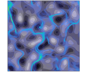
  $\varOmega >0$, white) and to the left of negative vortices (black). Panel (b) shows the same but for swimmers navigating a spatially smooth, steady random velocity field (see (2.5)). This suggests that the learnt strategy is robust, at least for steady two-dimensional flows, for parameter values similar to those shown in table 1.

Figure 3. (a)  $Q$ table of the optimal strategy when swimmers sense only
  $S_{nq}$. Each signal has three levels: negative (
 $-$), approximately zero (
 $0$) or positive (
 $+$), as described in § 2.3. The cells filled with blue indicate the optimal action for each state. (b) Typical trajectories of smart swimmers following the strategy shown in panel (a). Black dots represent the instantaneous position of the swimmer and the coloured line segments indicate the swimmer orientation
  $\boldsymbol n$ (representing the tail of the swimmer). The colours represent signals and corresponding actions: green,
  $S_{nq}<0$,
  $\omega _s<0$; red,
  $S_{nq}\approx 0$,
  $\omega _s=0$; salmon,
  $S_{nq}>0$,
  $\omega _s>0$. The background colour gives the normalised vorticity
  $2\varOmega _zL_0/u_0$. Remaining panels:
  $Q$ tables for different signal choices, using (c)
  $S_{nn} \text{ and } S_{nq}$; (d)
  ${\rm \Delta} u_q \text{ and } S_{nq}$ and (e)
  ${\rm \Delta} \varOmega \text{ and } S_{nq}$.

Figure 4. Number density  $N$ of swimmers following the dynamics (2.1) with angular swimming
  $\omega _{s}$ according to the strategy in figure 3(a) (colour scale) in (a) the TGV flow (2.3) and (b) the random velocity field (2.5). The grey background scale refers to the normalised fluid vorticity,
  $2\varOmega L_0/u_0$.
The underlying strategy in figure 3(a) relies entirely on the signal  $S_{nq}$. For a swimmer moving in a two-dimensional plane (the
  $x$–
$x$– $y$-plane), we have
 \begin{equation} S_{nq}=\boldsymbol{n}\boldsymbol{\cdot} {\mathbb{S}} \boldsymbol{q}\ = \boldsymbol{e}_z \boldsymbol{\cdot} [ \boldsymbol n \times ( \mathbb{S} \boldsymbol n)]. \end{equation}
Comparing with the equation of motion (see (2.1d)), we see that  $S_{nq}$ determines how the strain rotates the swimmer. When
  $S_{nq}$ is negative, for example, a prolate swimmer (
 $\varLambda >0$) is rotated clockwise by the strain. Figure 3(a) and (b) show that the optimal action does the same:
  $\omega _{s}<0$ means that the swimmer steers clockwise. For
  $S_{nq}>0$, however, the flow turns the swimmer counter-clockwise and so does the optimal action. Finally, when
  $S_{nq}$ is close to zero, the swimmer does not actively steer.
Because the steering mirrors the effect of the strain, we conclude that the swimmer tries to emulate a more slender swimmer, with a larger value of  $\varLambda$. This makes sense, because it was shown by Gustavsson et al. (Reference Gustavsson, Berglund, Jonsson and Mehlig2016) that naive gyrotactic swimmers (no steering actions,
  $\omega _{s}=0$) tend to sample upwelling regions of the flow when their shape factor
  $\varLambda$ increases, or at least regions where downwelling is weaker. In other words, the smart swimmers manage to preferentially sample upwelling regions of the flow by mimicking slender naive swimmers that take no steering actions (
 $\omega _{s}=0$). How this works is shown more quantitatively in figure 5, where we compare the performance of smart swimmers with
  $\varLambda =0.6$ to naive gyrotactic swimmers with
  $\varLambda \geq 0.6$. Figure 5 shows their mean vertical velocities
  $\langle v_y\rangle$, and also the different contributions to
  $\langle v_y\rangle$, namely
  $\langle n_y\rangle v_{s}$,
  $\langle u_y\rangle$ and the average vertical component of the settling velocity,
  $\langle \boldsymbol v_{g}\boldsymbol {\cdot } \boldsymbol e_{y}\rangle$. We see that the smart swimmers have an appreciable upward velocity, because gyrotaxis favours alignment between
  $\boldsymbol n$ and
  $\boldsymbol e_y$, and because the swimmers sample upwelling regions where
  $u_y >0$. Naive swimmers with the same value of
  $\varLambda$ also migrate upwards, but more slowly. Figure 5 reveals the reason: naive swimmers do not sample upwelling regions as efficiently as smart ones and do not align as much with the upward direction. Figure 5 also illustrates that naive swimmers with larger values of
  $\varLambda$ tend to sample upwelling regions more efficiently (
 $\langle u_y\rangle$ is larger) and align more with the upward direction than in the case
  $\varLambda =0.6$. For a spheroid, the shape factor
  $\varLambda$ is constrained to be smaller than unity (see (2.2)). It is nevertheless interesting to investigate the dynamics for larger values of
  $\varLambda$, artificially increasing the effect of the strain on the angular dynamics (Zhao et al. Reference Zhao, Gustavsson, Ni, Kramel, Voth, Andersson and Mehlig2019). Here, we change the value of
  $\varLambda$, but keep
  $\lambda$,
  $v_g^{\parallel }$ and
  $v_g^{\perp }$ constant, as given in table 1 (this means that (2.2) no longer holds).

Figure 5. Contributions to the vertical swimming of swimmers defined in case S6 (the leftmost group) and naive swimmers with different  $\varLambda$ (the other groups) in the TGV flow. The blue bars represent the average of vertical velocity
  $\langle v_y\rangle$. The red, yellow and purple bars represent the vertical velocity owing to swimming, advection of local fluid and settling, respectively. All velocities are normalised by the swimming velocity
  $v_{s}$.
Figure 5 shows that a smart swimmer with shape factor  $\varLambda =0.6$ migrates as fast as a naive swimmer with
  $\varLambda = 1.2$, roughly twice as fast as a naive swimmer of the same parameter
  $\varLambda =0.6$. We see that the average vertical velocity
  $\langle v_y\rangle$ increases as
  $\varLambda$ grows until
  $\varLambda =2$. This is explained by three observations. First, the average vertical swimming velocity
  $\langle n_y\rangle v_s$ increases as
  $\varLambda$ increases from 0.6 to 1.4, because
  $\boldsymbol n$ tends to align with
  $\boldsymbol e_y$. However, note that the alignment becomes weaker for
  $\varLambda >1.4$. Second, as predicted by Gustavsson et al. (Reference Gustavsson, Berglund, Jonsson and Mehlig2016) and later verified by direct numerical simulations of turbulence (Borgnino et al. Reference Borgnino, Boffetta, De Lillo and Cencini2018; Cencini et al. Reference Cencini, Boffetta, Borgnino and De Lillo2019; Lovecchio et al. Reference Lovecchio, Climent, Stocker and Durham2019), the dynamics of gyrotactic swimmers undergoes a flow-and-parameter dependent transition from preferential sampling of downwelling regions for
  $\varLambda <\varLambda _{c}$ to upwelling regions for
  $\varLambda >\varLambda _{c}$. For the TGV flow and parameters leading to figure 5, this transition occurs at
  $\varLambda _{c}\approx 1$, as shown in figure 5. This implies that naive gyrotactic swimmers cannot sample upwelling regions. Smart swimmers, however, succeed in sampling upwelling regions by emulating naive swimmers with
  $\varLambda >1$. Third, the settling velocity
  $\langle \boldsymbol v_{g}\boldsymbol {\cdot } \boldsymbol e_{y}\rangle$ is found to be almost independent of
  $\varLambda$. This is explained by the observation that the orientation
  $\boldsymbol n$ has only a small influence on the settling velocity because
  $v_{g}^{\parallel }$ and
  $v_{g}^\perp$ are of the same order of magnitude for the parameters given in table 1. These three observations explain the strategy shown in figure 3(a), as well as the trajectory patterns shown in figures 3(b) and 4.
Up to now, we discussed the simplest case, where the swimmers sense only one signal,  $S_{nq}$ (figure 3(a)). Now consider the cases where the swimmers sense not only
  $S_{nq}$ but also other signals. In each case, we obtain an efficient strategy as shown in figure 3(c–e). These strategies are robust, because they are learnt in both TGV flow and a random velocity field. However, these strategies are only slightly better than the one in figure 3(a): the resulting upward velocities are of the same order of magnitude for all the four strategies (figure 7). Moreover, these strategies share a similar pattern. For instance, the strategy in figure 3(c) yields actions independent of the signal
  $S_{nn}$. In other words, it is identical to the strategy obtained using only
  $S_{nq}$ as a signal (figure 3(a)). For the cases where the swimmers measure
  ${\rm \Delta} u_q$ or
  ${\rm \Delta} \varOmega$ in addition to
  $S_{nq}$, the
  $Q$ tables shown in panels (d) and (e) illustrate that
  ${\rm \Delta} u_q$ is useful only when
  $S_{nq}$ is close to zero, and
  ${\rm \Delta} \varOmega$ is useful only when
  $S_{nq}$ and
  ${\rm \Delta} \varOmega$ are either both positive or negative. This means measuring extra signals in addition to
  $S_{nq}$ provides not much more useful information for the upward navigation of swimmers. We therefore conclude that it is
  $S_{nq}$ that provides the most important information, because in two-dimensional flows, it is a direct measure of the rotation the fluid strain exerts upon the swimmer and it allows the swimmers to smartly mimic more elongated swimmers.
4. Conclusions
We analyse how a micro-swimmer can navigate a complex flow relying only on local hydrodynamic signals. We assume that the swimmer can actively rotate in its frame of reference in response to the local signals. Using reinforcement learning, we found that successful swimming strategies exist only if the swimmer can distinguish the target direction. The flows we considered do not provide direct information concerning the target: the TGV flow has  $C_4$ symmetry and the random velocity field is statistically isotropic. As a consequence, both velocity fields exhibit vertical reflection symmetry. In this case, the dynamics must break vertical reflection symmetry to allow the reinforcement learning algorithm to find meaningful strategies. For example, gravity breaks this symmetry because it causes gyrotaxis or settling and this allows the swimmer to navigate with local signals and actions. For the case of settling owing to gravity, we found that even though settling opposes the migration task, the resulting breaking of vertical reflection symmetry allows the swimmer to swim upwards with an average velocity larger than the settling velocity.
We investigate the underlying mechanism of navigation with local signals by considering swimmers with both gyrotaxis and settling. Reinforcement learning projects out a simple but efficient optimal strategy for vertical navigation: the swimmer measures the strain component,  $S_{nq}$, allowing it to adjust its angular velocity to amplify strain-mediated rotations, which leads to a preferential sampling of strain regions and upwelling regions. For the parameters tested here, we found the same optimal strategy in both the TGV flow and different realisations of a smooth random velocity field, which indicates that the strategy is robust. For the tested cases, the strategy leads to twice the navigation speed compared with a naive gyrotactic swimmer (Kessler Reference Kessler1985; Durham et al. Reference Durham, Climent and Stocker2011, Reference Durham, Climent, Barry, De Lillo, Boffetta, Cencini and Stocker2013; Gustavsson et al. Reference Gustavsson, Berglund, Jonsson and Mehlig2016).
In this article, we use a highly idealised model for a micro-swimmer to investigate the role of symmetries in  $Q$-learning using local signals. To speculate in how far the model may apply to any given planktonic micro-organism, the model assumptions must be critically assessed. First, it is assumed that the micro-swimmer is rigid and that the swimmer swims with a constant speed. This rules out jumping copepods escaping predators, but may apply to cruising swimmers. Copepods, for example, can cruise by moving their appendages in specific, high-frequency gaits (Jiang et al. Reference Jiang, Osborn and Meneveau2002). Dinoflagellates can also cruise using their flagella (Kamykowski, Reed & Kirkpatrick Reference Kamykowski, Reed and Kirkpatrick1992). Second, we assume that the micro-swimmer can measure local fluid strain, as well as its relative rotation and its relative translation to the fluid. This is in principle possible with setae or cilia, as for copepods (Kiørboe et al. Reference Kiørboe, Saiz and Visser1999), ciliates (Jakobsen Reference Jakobsen2001), rotifers (Kirk & Gilbert Reference Kirk and Gilbert1988) and invertebrate larvae (Mackie et al. Reference Mackie, Singla and Thiriot-Quievreux1976; Fuchs et al. Reference Fuchs, Hunter, Schmitt and Guazzo2013). More signals provide more information, facilitating navigation. This suggests that the swimming strategies of a realistic swimmer may rely on all available signals, possibly including light and chemical concentration gradients in addition to hydrodynamic signals. Third, we assume the swimmer is rigid and that hydrodynamic signals are unaffected by the motion of the swimmer. This is because a micro-swimmer is thought to be able to distinguish external fluid disturbance from that generated by its own motion (Hwang & Strickler Reference Hwang and Strickler2001) by recognising temporal and spatial characteristics of signals (Yen & Strickler Reference Yen and Strickler1996; Fields Reference Fields2014). However, realistic swimmers need to deform smartly to propel (Verma, Novati & Koumoutsakos Reference Verma, Novati and Koumoutsakos2018; Tsang et al. Reference Tsang, Tong, Nallan and Pak2020; Hartl et al. Reference Hartl, Hb l, Kahl and Zẗtl2021). The interaction between the swimmer and fluid must disturb the local flow field, which makes it more difficult to measure external signals. How and to what extent a swimmer can extract useful signals remain to be investigated. Fourth, our results are obtained for the parameters given in table 1. Although the mechanisms found here are robust to small parameter changes (figure 7 in Appendix A), it is clear that the found strategies must fail when the parameters change substantially. For example, we choose
  $\omega _{s}$ to be five times larger than the gyrotactic angular velocity of the order of
  $B^{-1}$, which facilitates the control of swimming direction. Whether there exist efficient navigation strategies when
  $\omega _{s}$ is small compared with
  $B^{-1}$ remains an open question. As another example, for much larger swimming speeds, the preferential sampling becomes weaker (Gustavsson et al. Reference Gustavsson, Berglund, Jonsson and Mehlig2016), so that it becomes harder to outperform the naive strategy (Colabrese et al. Reference Colabrese, Gustavsson, Celani and Biferale2017).
In our model, we consider steady flows in two spatial dimensions. Our idealised flow configurations allow us to investigate the symmetry problem and the underlying mechanism of hydrodynamic signal in an intuitive way. When generalised to more realistic situations, the breaking of symmetry is also important. For example, symmetry needs to be broken for a swimmer to navigate through locally isotropic turbulence in the ocean. However, the optimal strategies are expected to be different in a three-dimensional and time-dependent flow, because three-dimensional dynamics is more complex and brings additional flow signals to act upon. It remains an open question to determine optimal strategies in three-dimensional unsteady flows. Moreover, in our model, the perceived signals were given by estimated threshold values in table 2, but in reality, the swimmers may respond to other levels of hydrodynamic signals. How can we determine which level is the most important? Is it possible to model the signal under disturbances from swimming?
Optimising the rate of vertical migration is a fairly simple task, and this choice of target allowed us to study the effect of symmetry breaking, and to compare with the existing literature on navigation of smart swimmers (Colabrese et al. Reference Colabrese, Gustavsson, Celani and Biferale2017). However, in nature, there are competing tasks, such as minimising energy consumption during migration or avoiding predation (Huntley & Brooks Reference Huntley and Brooks1982; Morris, Gust & Torres Reference Morris, Gust and Torres1985; Park et al. Reference Park, Jeong, Lee, Cho and Kwon2001). How to analyse the effects of these competing tasks remains an open question, necessary to answer to understand observed survival strategies of motile micro-organisms in the ocean.
Funding
K.G. and B.M. are supported in part by a grant from the Knut and Alice Wallenberg Foundation, grant no. 2019.0079, and in part by VR grant no. 2017-3865. K.G. is supported by Vetenskapsrådet, Grant No. 2018-03974. B.M. and L.Z. are supported by a collaboration grant from the joint China–Sweden mobility programme (National Natural Science Foundation of China (NSFC)–Swedish Foundation for International Cooperation in Research and Higher Education (STINT)), grant nos. 11911530141 (NSFC) and CH2018-7737 (STINT). J.Q. and L.Z. acknowledge the support from the Institute for Guo Qiang of Tsinghua University (Grant No. 2019GQG1012). C.X. acknowledges the support from NSFC (Grant No. 91752205).
Declaration of interest
The authors report no conflict of interest.
Appendix A. Numerical details
In this appendix, we give details of the different simulations summarised in table 3 and the implementation of the reinforcement learning algorithm.
To implement the  $Q$-learning algorithm, both actions and states are discretised. The action is to modify the angular swimming velocity
  $\boldsymbol \omega _{s}$ in (2.1d). In cases S1, S2, S4, S5 and S6, the actions are given by (2.7). In case S3, the actions are given by (2.8), with
  $\boldsymbol k$ being one of
  $(0,-1,0)$,
  $(1,0,0)$,
  $(0,1,0)$ or
  $(-1,0,0)$ (Colabrese et al. Reference Colabrese, Gustavsson, Celani and Biferale2017). The states are given by different combinations of the signals. In cases S1, S3, S4 and S5, the states are given by the combination of
  $S_{nn}$ and
  $S_{nq}$. In case S2, the states are given by the combination of three levels of local vorticity
  $\varOmega$ and four discrete levels of the instantaneous direction
  $\boldsymbol n$ of the swimmer (Colabrese et al. Reference Colabrese, Gustavsson, Celani and Biferale2017). In case S6, the states are given either by the signal
  $S_{nq}$ solely or in combination with one of
  $S_{nn}$,
  ${\rm \Delta} u_q$ and
  ${\rm \Delta} \varOmega$ (see (2.6)).
The training with reinforcement learning is divided into episodes. In each episode, ten swimmers are initialised with random locations and orientations, and simulated to update the  $Q$ table in parallel. The Gaussian noises
  $\boldsymbol \xi$ and
  $\boldsymbol \eta$ in (2.1b) and (2.1d) are implemented at every time step by Gaussian translational and rotational displacements with variances
  $\sqrt {2D_t {\rm \Delta} t}$ and
  $\sqrt {2D_r {\rm \Delta} t}$, respectively, where
  $D_t = 0.001L_0 u_0$ and
  $D_r = 0.01u_0/L_0$. For the simulation in the TGV flow, we integrate (2.1) numerically using an explicit second-order Adams–Bashforth scheme for
  $10^5$ time steps of size
  ${\rm \Delta} t = 0.01u_0/L_0$, which allows for the position, velocity and orientation of the swimmer to reach a statistically steady state. The state
  $s_i$ of a given swimmer is evaluated and the
  $Q$ table is updated every 10 time steps, which results in a total of
  $i_{max} = 10^4$ state updates in each episode. We use
  $\gamma = 0.999$, which corresponds to a time window of order
  $(1-\gamma )^{-1}=10^3$ state changes or
  $25\ \text {s}$ in physical time. This time window is much longer than the time scale for a swimmer to move through a vortex, estimated by
  $L_0/v_{s} = 0.5\ \text {s}$.
We make similar assumptions and choose similar parameters for our simulations using random velocity fields, but there are a number of minor differences. First, the state  $s_i$ is evaluated at every time step but the
  $Q$ table is updated only when the state changes. Second, each episode lasts for 2500 s, which corresponds to at least
  $i_{max} = 10^4$ state changes. Third, we use the Euler method to integrate (2.1), rather than the Adams–Bashforth scheme. We confirm that the two approaches yield the same results for the TGV flow.
During training, we take both the learning rate,  $\alpha$, and the exploration rate,
  $\varepsilon$, to decrease as the episode number
  $j$ increases, i.e.
 \begin{equation} \alpha=\alpha_0\frac{\sigma_0}{\sigma_0+j}, \quad \varepsilon=\varepsilon_0 \max\left(0, 1- {\frac{j}{j_0}} \right), \end{equation}
with initial learning and exploration rates  $\alpha _0$ and
  $\varepsilon _0$ and decay scales
  $\sigma _0$ and
  $j_0$. Training parameters for all cases are shown in table 4.
Table 4. Training parameters.

We use the total reward,  $R = \sum _{i=0}^{i_{max}}r_i L_0 /T_Nv_s$, to evaluate the performance of strategies found during training, where
  $r_i$ is the reward of each state change defined in (2.9) and
  $i_{max}$ is the total number of state changes in a single episode. The
  $R$ indicates how fast a swimmer navigates upward. We note that
  $R$ is different from the concept of discounted reward, as mentioned in § 2.4. The training has converged when
  $\varSigma _r$ has reached a plateau (figure 6).

Figure 6. Evolution of the total reward  $R$ as a function of episode. The curves represent the moving average of
  $R$ over 100 episodes. Each panel shows 5 different learning processes.
To test the robustness of the strategies shown in figure 3, we examined the strategies on swimmers whose parameter values are perturbed from table 1. The vertical velocities of swimmers shown in figure 7 show that the optimal strategies are robust to moderate changes of the parameters and better than the naive strategy in most of cases.

Figure 7. Robustness of strategies to small parameter perturbations. (a) TGV flow and (b) random velocity field. P1, result for parameters given in table 1. P2, same, but  $v_s = 2.0$ mm s
 $^{-1}$. P3,
  $v_s = 0.5$ mm s
 $^{-1}$. P4,
  $\omega _s = 1.2$ rad s
 $^{-1}$. P5,
  $\omega _s = 0.8$ rad s
 $^{-1}$. P6,
  $S_c = 0.8\ \text {s}^{-1}$.


