


1. Introduction
Combustion instabilities (CIs) and combustion noise continue to pose a significant problem during the development and operation of gas turbines and flight engines operated in the lean, premixed combustion regime (Poinsot Reference Poinsot2017). One mechanism that can lead to CIs are inhomogeneities in fuel–air mixing, which originate at the fuel injector (Lieuwen & Zinn Reference Lieuwen and Zinn1998). These inhomogeneities are subsequently convected, e.g. in a mixing duct, towards the flame front. There, they interact with the flame, causing heat release fluctuations (Lieuwen, Neumeier & Zinn Reference Lieuwen, Neumeier and Zinn1998). These in turn create acoustic energy, which may feed back into a thermoacoustic feedback cycle or add to combustion noise. The evolution mechanisms and impact of this effect on the flame dynamics were extensively analysed using experiments (e.g. Shih, Lee & Santavicca Reference Shih, Lee and Santavicca1996; Lieuwen et al. Reference Lieuwen, Neumeier and Zinn1998; Venkataraman et al. Reference Venkataraman, Preston, Simons, Lee, Lee and Santavicca1999; Bluemner, Paschereit & Oberleithner Reference Bluemner, Paschereit and Oberleithner2019) as well as numerical high-fidelity simulations (e.g. Huber & Polifke Reference Huber and Polifke2009a,Reference Huber and Polifkeb; Hermeth et al. Reference Hermeth, Staffelbach, Gicquel and Poinsot2013).
When interacting with the flame front, fuel ratio inhomogeneities are furthermore the main cause of the evolution of entropy waves (Dowling & Stow Reference Dowling and Stow2003; Chen, Bomberg & Polifke Reference Chen, Bomberg and Polifke2016), i.e. pockets of higher or lower temperature in the burnt gases. These pockets are then transported by the flow towards the turbine stages. This process constitutes another unwanted effect, since entropy waves increase nitrous oxide emissions (Martin & Brown Reference Martin and Brown1990; Shih et al. Reference Shih, Lee and Santavicca1996) and furthermore cause acoustic perturbations as they are accelerated at the first stator stage of the turbine (Bohn Reference Bohn1976; Marble & Candel Reference Marble and Candel1977). These acoustic perturbations may either feed back in a thermoacoustic cycle (Polifke, Paschereit & Döbbeling Reference Polifke, Paschereit and Döbbeling2001; Goh & Morgans Reference Goh and Morgans2013; Motheau, Nicoud & Poinsot Reference Motheau, Nicoud and Poinsot2014; Morgans & Duran Reference Morgans and Duran2016) or emanate from the combustion chamber as indirect combustion noise and contribute to the overall noise emission of the engine (Cumpsty, Marble & Hawthorne Reference Cumpsty, Marble and Hawthorne1977; Strahle Reference Strahle1978), a problem of increasing significance, especially in aeroengines (Dowling & Mahmoudi Reference Dowling and Mahmoudi2015). Like the effect of fuel ratio inhomogeneities, the evolution process of entropy waves and their impact on the thermoacoustic stability of the engine have been investigated by various experimental (Ćosić et al. Reference Ćosić, Terhaar, Moeck and Paschereit2015; Wassmer et al. Reference Wassmer, Schuermans, Paschereit and Moeck2017) and numerical studies (Morgans, Goh & Dahan Reference Morgans, Goh and Dahan2013; Xia et al. Reference Xia, Duran, Morgans and Han2018).
While experimental and high-fidelity computational fluid dynamics (CFD) enable us to observe the evolution and effect of entropy waves, they remain very elaborate and conclusions on how to control the effect remains a matter of trial and error. Analytical models, on the other hand, allow us to investigate the effect of changing key parameters in the combustion system. For example, models were developed to describe and understand the origin, convection and effect of entropy waves (e.g. Marble & Candel Reference Marble and Candel1977; Moase, Brear & Manzie Reference Moase, Brear and Manzie2007). As pointed out by Sattelmayer (Reference Sattelmayer2002), these prior studies model the convection of entropy waves by a constant velocity. This is equivalent to considering a block velocity profile in the combustor, an assumption which is not sustainable in a real engine, where a non-homogeneous mean flow profile causes destructive interference of entropy fluctuations at the measuring point, a process termed mean flow shear dispersion by Sattelmayer (Reference Sattelmayer2002). The same author found this effect to be especially strong in flows exhibiting a large variety in convective time delays. To model this effect in network models, the author furthermore suggested a transfer function (TF) to measure convection of entropy waves. The TF is based on a fit of a rectangular impulse response (IR) to empirical data. By fitting a Gaussian curve instead of a rectangular IR to the empirical data, Morgans et al. (Reference Morgans, Goh and Dahan2013) developed this low-order model further and compared its results to direct numerical simulation (DNS), in which they included a transport equation of a passive scalar to account for the transport of entropy waves. In a related study, Giusti et al. (Reference Giusti, Worth, Mastorakos and Dowling2017) found that, for low frequencies, a model accounting for shear layer dispersion correctly describes the decrease of the passive scalar TF with increasing frequency. For higher frequencies, however, their model overestimates the empirical TF. They concluded that turbulent diffusion, which is not taken into account in their model, must account for the difference. Moreover, recent studies show that the frequency range in which turbulent transport plays a significant role in the convection of entropy waves Xia et al. (Reference Xia, Duran, Morgans and Han2018) and fuel ratio fluctuations Bluemner et al. (Reference Bluemner, Paschereit and Oberleithner2019) overlaps with the typical frequency range of thermoacoustic instabilities. Hence, to improve the capability of thermoacoustic stability prediction, turbulent transport should be taken into consideration in reduced-order models.
In order to take molecular and turbulent diffusion into account and re-evaluate their impact on the overall convection process, this study aims at applying linearization of the governing equations of the flow. Linearization is a well-established approach in the context of linear stability analysis (LSA) and resolvent analysis (RA). (The readers interested in details on the concept of RA are kindly referred to the respective literature, e.g. McKeon & Sharma (Reference McKeon and Sharma2010), Beneddine et al. (Reference Beneddine, Sipp, Arnault, Dandois and Lesshafft2016) and Kaiser, Lesshafft & Oberleithner (Reference Kaiser, Lesshafft and Oberleithner2019a).) In the past, these methods provided significant insight into phenomena in various fields of fluid dynamics. At the same time, the necessary numerical expenses related to LSA and RA are, for most configurations, closer to the ones of analytical models than to the aforementioned high-fidelity CFD methods. Nevertheless, the treatment of turbulent mass diffusion in the transport of a passive scalar in the linear framework remains unaddressed up to this point. Recent studies show that, in LSA (e.g. Crouch, Garbaruk & Magidov Reference Crouch, Garbaruk and Magidov2007; Oberleithner, Paschereit & Wygnanski Reference Oberleithner, Paschereit and Wygnanski2014; Viola et al. Reference Viola, Iungo, Camarri, Porté-Agel and Gallaire2014; Tammisola & Juniper Reference Tammisola and Juniper2016; Kaiser et al. Reference Kaiser, Oberleithner, Selle and Poinsot2019b) and RA (e.g. Illingworth, Monty & Marusic Reference Illingworth, Monty and Marusic2018; Pickering et al. Reference Pickering, Rigas, Sipp, Schmidt and Colonius2019; Kaiser et al. Reference Kaiser, Lesshafft and Oberleithner2019a; Martini et al. Reference Martini, Cavalieri, Jordan, Towne and Lesshafft2020), the effect of turbulent momentum diffusion can be taken into account via a turbulent contribution to viscosity. Recently, Morra et al. (Reference Morra, Semeraro, Henningson and Cossu2019) showed that the use of an eddy viscosity significantly improves the capability of the RA in predicting the turbulent power spectral density in the near wall region.
The advancements of linearized methods in modelling turbulent momentum transport are the motivation for the present investigation, which aims at addressing the applicability of a similar approach for the turbulent mass transport of the passive scalar. The presently derived method requires the temporal mean flow as input. It is obtained from the DNS conducted by Morgans et al. (Reference Morgans, Goh and Dahan2013), which will also serve as a validation basis for the results of the linear approach.
While aiming to address physical phenomena in real combustion systems, the previous analytical studies were restricted to fully developed flows in tubes or channels and assumed that turbulent mixing can be neglected. Flows in real gas turbines, however, are significantly more complicated. Multiple shear layers due to vortex breakdown, enhanced turbulence due to swirl and high Reynolds numbers hinder a rigorous application of the state-of-the-art analytic models. The method proposed here is not restricted to simple configurations, as it builds on less strong assumptions. Therefore, if validated successfully against the existing analytical models, the proposed method constitutes a step forward from canonical flow cases to real world applications.
In this study, a passive scalar is used to model the convective transport of entropy fluctuations in the combustion chamber, which implies the assumption of constant density and thermophysical properties. Although the typical length scales (and therefore frequencies) differ from those from entropy waves, the very same approach can be used to model the convection of fuel ratio inhomogeneities in the mixing duct towards the flame (e.g. Bluemner et al. Reference Bluemner, Paschereit and Oberleithner2019). For the sake of generality and simplicity, from here on this paper will therefore use the term passive scalar to refer to both quantities, i.e. fuel mixture and entropy.
This paper is organized as follows: § 2 reviews the DNS of the turbulent channel flow performed by Morgans et al. (Reference Morgans, Goh and Dahan2013) and selected low-order models. In § 3 the linearized equation of the passive scalar is derived, the turbulence closure is addressed and the numerical implementation is outlined. In § 4 the linearized methodology is validated against the DNS and the impact of molecular and turbulent diffusion and mean flow shear dispersion on the convection is quantified. Finally, § 5 concludes the results.
2. Current transport models exemplified for a turbulent channel flow
The linearized study in this paper is based on the DNS calculations of a fully developed channel flow at a Reynolds number of  ${Re}= 3400$, conducted by Moser, Kim & Mansour (Reference Moser, Kim and Mansour1999) (accessible online at Moser, Kim & Mansour Reference Moser, Kim and Mansour1998), which was repeated by Morgans et al. (Reference Morgans, Goh and Dahan2013) to include the transport of a passive scalar,
  $c$. The DNS domain is schematically illustrated in figure 1. The wall-to-wall distance in the channel is
  $2 h$, and the channel length and width are
  $2{\rm \pi} h$ and
  ${\rm \pi} h$, respectively. The passive scalar field in the DNS was pulsed at the inlet. Subsequently, Morgans et al. (Reference Morgans, Goh and Dahan2013) quantified the convection of the passive scalar fluctuation via a linear-time-invariant (LTI) system, which relates the cross-streamwise integrals of the passive scalar fluctuation at two different streamwise locations,
  $x_1$ and
  $x_2$. If not mentioned otherwise,
  $x_1$ and
  $x_2$ are located at the inlet and outlet, respectively. The TF of the LTI system is defined as
 \begin{equation} \text{TF} \left({St}\right)=\frac{\displaystyle\iint\hat{c}\left( x_1\right) {\textrm{d} y}\, \textrm{d}z}{ \displaystyle\iint \hat{c}\left( x_2\right) {\textrm{d} y} \,\textrm{d}z},\end{equation}
where the caret superscript stands for a Fourier transform in time. The Strouhal number in (2.1) is a non-dimensionalized frequency, defined as
 \begin{equation} {St} = \frac{f L}{U}, \end{equation}
where  $f$ is the frequency,
  $L$ the length of the channel and
  $U$ the bulk flow velocity. The IR and the TF of a LTI system in general are connected by the
  $z$-transform. For convenience, in this paper signals are treated as time discrete. Therefore, the term
  $z$-transform is used instead of Laplace transform.

Figure 1. Sketch of the DNS domain of Morgans et al. (Reference Morgans, Goh and Dahan2013) and the strategy to measure the convection of passive scalar fluctuations via TF and IR.
The solid black lines in the two diagrams shown in figure 1 represent the results of the DNS conducted by Morgans et al. (Reference Morgans, Goh and Dahan2013). The response in time domain shown on the right is the response measured at the outlet to a Gaussian pulsation at the inlet and is, therefore, not the IR of the system, but only an approximation. Morgans et al. (Reference Morgans, Goh and Dahan2013) fit two models to this IR. The first is the one suggested by Sattelmayer (Reference Sattelmayer2002), which models the response as a rectangular signal (red dotted line in figure 1). The second fit is suggested by Morgans et al. (Reference Morgans, Goh and Dahan2013) and assumes a Gaussian profile for the response (blue dash-dotted line in figure 1). The quality of the fits can be evaluated by comparing the TFs of the respective models, which are obtained by a  $z$-transform of the IRs, to the TF directly extracted from the DNS. The comparison shows that both models reproduce the overall shape of the gain of the TF based on the DNS, which starts at
  $1$ and decreases with frequency. However, both models overestimate the gain for low frequencies and for high frequencies, the Sattelmayer model, due to the abrupt jumps in the IR, shows ripples, which are not seen in the DNS. Furthermore, for high frequencies, the model suggested by Morgans et al. (Reference Morgans, Goh and Dahan2013) significantly underestimates the DNS results. While the previous models are purely based on empirical data, Giusti et al. (Reference Giusti, Worth, Mastorakos and Dowling2017) suggested an analytical model, which takes the advection of the passive scalar due to the temporal mean flow into account. In doing so, it accounts for mean flow shear dispersion, while molecular and turbulent mass transport are neglected. Furthermore, the method of Giusti et al. (Reference Giusti, Worth, Mastorakos and Dowling2017) is applicable only to fully developed flows. The respective curve is illustrated in figure 1 (solid grey line). This model will be more thoroughly discussed in § 4. While for low frequencies, pure mean flow shear dispersion appears to capture the decrease in the TF gain seen in the DNS, the model clearly overestimates the TF gain at high frequencies. Giusti et al. (Reference Giusti, Worth, Mastorakos and Dowling2017) attribute this overestimation to turbulent diffusion, which is not captured in their model. As a consequence, the following section will investigate how diffusive processes can be modelled in a linearized framework.
3. Linearization of the transport equations around the temporal mean
Following the approach of previous authors (e.g. Morgans et al. Reference Morgans, Goh and Dahan2013), the entropy and equivalence ratio are modelled by a passive scalar,  $c$. Taking the effect of molecular diffusion into account, its transport equation reads
 \begin{equation} \frac{\partial c}{\partial t} + \boldsymbol{\nabla} \boldsymbol{\cdot} \left(\boldsymbol{u} c\right) = \boldsymbol{\nabla} \boldsymbol{\cdot} D_{m} \boldsymbol{\nabla} c ,\end{equation}
where  $t$ is time,
  $\boldsymbol {u}$ the velocity vector and
  $D_{m}$ stands for molecular diffusivity.
The triple decomposition suggested by Hussain & Reynolds (Reference Hussain and Reynolds1970) allows us to address the dynamics of coherent fluctuations in the presence of turbulence. It decomposes the flow variables into a temporal average, a periodically fluctuating part and a stochastically fluctuating part, indicated by the superscripts bar, tilde and prime, respectively, reading
 \begin{equation} \boldsymbol{u} = \bar{\boldsymbol{u}} + \tilde{\boldsymbol{u}} + \boldsymbol{u}^\prime,\quad c = \bar{c} + \tilde{c} + c^\prime.\end{equation}
The periodic fluctuation is defined such that, for a quantity  $\varPhi$, the relation
 \begin{equation} \langle \varPhi \rangle = \bar{\varPhi} + \tilde{\varPhi}\end{equation}
holds, where the angle brackets denote a phase average.
Inserting (3.2a,b) into (3.1), neglecting second-order terms of periodic fluctuation quantities and subtracting the temporal average of the resulting equation (indicated by an overline superscript) from its phase average yields the equation governing the linear dynamics of the passive scalar
 \begin{equation} \frac{\partial \tilde{c}}{\partial t} + \boldsymbol{\nabla} \boldsymbol{\cdot} \left(\bar{\boldsymbol{u}} \tilde{c} \right) + \boldsymbol{\nabla} \boldsymbol{\cdot} \left(\tilde{\boldsymbol{u}} \bar{c} \right) +\boldsymbol{\nabla} \boldsymbol{\cdot} \langle {\boldsymbol{u}}^\prime{c}^\prime \rangle -\boldsymbol{\nabla} \boldsymbol{\cdot} \overline{{\boldsymbol{u}}^\prime {c}^\prime} = \boldsymbol{\nabla} \boldsymbol{\cdot} D_{m} \boldsymbol{\nabla} \tilde{c}.\end{equation}
The term on the right-hand side describes molecular diffusion. The first term on the left-hand side accounts for the oscillation of the periodic passive scalar fluctuation in time. The second term governs the convection of the periodic fluctuation in the passive scalar due to the temporal mean flow. The third term on the left-hand side describes the production of  $\tilde {c}$ due to the interaction of the periodic velocity fluctuation with the temporally averaged passive scalar field. For the sake of comparability with previous analyses, in this work no periodic fluctuations in velocity are considered and, therefore, the third term vanishes. The fourth and fifth terms are product terms of stochastic fluctuations, which originate from the advective term in (3.1) and do not vanish after phase or temporal averaging. Using (3.3), the difference of both terms as it arises in (3.4) can be rewritten as
 \begin{equation} \boldsymbol{\nabla} \boldsymbol{\cdot} \langle {\boldsymbol{u}}^\prime{c}^\prime \rangle -\boldsymbol{\nabla} \boldsymbol{\cdot} \overline{{\boldsymbol{u}}^\prime {c}^\prime} = \boldsymbol{\nabla} \boldsymbol{\cdot} \widetilde{\boldsymbol{u}^\prime c^\prime}, \end{equation}
which shows that it can be understood as the periodic fluctuation of  $\boldsymbol {\nabla } \boldsymbol {\cdot } (\boldsymbol {u}^\prime c^\prime )$. The same assessment has been made for the fluctuation of Reynolds stresses arising in the linearized momentum conservation equations by Reynolds & Hussain (Reference Reynolds and Hussain1972).
To close (3.4), the fourth and fifth terms on the left-hand side remain to be modelled. Using the gradient diffusion hypothesis (Pope Reference Pope2000), we relate these terms to the gradient of the averaged passive scalar via a turbulent diffusion  $D_{t}$, which reads
 \begin{gather} \overline{ \boldsymbol{u}^\prime c^\prime} ={-} D_{t}^{m} \boldsymbol{\nabla} \bar{c}, \end{gather}
 \begin{gather}\langle \boldsymbol{u}^\prime c^\prime \rangle ={-} D_{t}^{p} \boldsymbol{\nabla} \langle c \rangle, \end{gather}
for the temporal and phase averages, respectively.
To analyse the relation between turbulent diffusivity related to the temporal mean,  $D_{t}^{m}$, and the turbulent diffusivity for the phase average,
  $D_{t}^{p}$, we follow the approach of Viola et al. (Reference Viola, Iungo, Camarri, Porté-Agel and Gallaire2014). They performed an equivalent analysis for the turbulent viscosity in the conservation equations of momentum, by linearizing the turbulent viscosity,
  $\nu _{t}^{p}$.
In order to linearize  $D_{t}^{p}$ with respect to
  $\tilde {c}$ and
  $\tilde {\boldsymbol {u}}$,
  $D_{t}^{p}$ is expanded as a Taylor series around the temporal average and all terms of second and higher order are neglected
 \begin{equation} D_{t}^{p}\left( \bar{\boldsymbol{u}} + \tilde{\boldsymbol{u}}, \bar{c} + \tilde{c} \right) \approx D_{t}^{p}\left( \bar{\boldsymbol{u}}, \bar{c} \right) +\frac{\partial D_{t}^{p}\left( \bar{\boldsymbol{u}}, \bar{c} \right)}{\partial \boldsymbol{u}} \boldsymbol{\cdot} \tilde{\boldsymbol{u}} +\frac{\partial D_{t}^{p}\left( \bar{\boldsymbol{u}}, \bar{c} \right)}{\partial c} \tilde{c}.\end{equation}
Inserting (3.7) in (3.6b) and averaging the resulting equation in time yields
 \begin{align} \overline{\boldsymbol{u}^\prime c^\prime} &={-}{D_{t}^{p}\left( \bar{\boldsymbol{u}}, \bar{c} \right) \boldsymbol{\cdot} \boldsymbol{\nabla} \bar{c} } -\overline{D_{t}^{p}\left( \bar{\boldsymbol{u}}, \bar{c} \right) \boldsymbol{\cdot} \boldsymbol{\nabla} \tilde{c} } -\overline{\left(\frac{\partial D_{t}^{p}\left( \bar{\boldsymbol{u}}, \bar{c} \right)}{\partial \boldsymbol{u}} \boldsymbol{\cdot} \tilde{\boldsymbol{u}} \right) \boldsymbol{\cdot} \boldsymbol{\nabla} \bar{c} }\nonumber\\ &\quad -\overline{\left(\frac{\partial D_{t}^{p}\left( \bar{\boldsymbol{u}}, \bar{c} \right)}{\partial \boldsymbol{u}} \boldsymbol{\cdot} \tilde{\boldsymbol{u}} \right) \boldsymbol{\cdot} \boldsymbol{\nabla} \tilde{c}} -\overline{\left(\frac{\partial D_{t}^{p}\left( \bar{\boldsymbol{u}}, \bar{c} \right)}{\partial c} \tilde{c} \right) \boldsymbol{\cdot} \boldsymbol{\nabla} \bar{c} } -\overline{\left(\frac{\partial D_{t}^{p}\left( \bar{\boldsymbol{u}}, \bar{c} \right)}{\partial c} \tilde{c} \right) \boldsymbol{\cdot} \boldsymbol{\nabla} \tilde{c} }. \end{align}
On the right-hand side of (3.8), the second, third and fifth terms are zero due to the temporal average, while the fourth and sixth terms are nonlinear in quantities of periodic fluctuation and are therefore neglected. As a consequence, on the right-hand side only the first term remains. Comparing this result to (3.6a) yields that  $D^{m}_{t}$ and
  $D^{p}_{t}$ are identical in the linear limit and the superscripts
  ${m}$ and
  ${p}$ can be dropped in the following. With the relation
  $\langle c \rangle - \bar {c}=\tilde {c}$, inserting (3.6) into (3.4) finally yields
 \begin{equation} \frac{\partial \tilde{c}}{\partial t} + \boldsymbol{\nabla} \boldsymbol{\cdot} \left(\bar{\boldsymbol{u}} \tilde{c} \right) + \boldsymbol{\nabla} \boldsymbol{\cdot} \left(\tilde{\boldsymbol{u}} \bar{c} \right) = \boldsymbol{\nabla} \boldsymbol{\cdot} \left( D_{m} + D_{t} \right) \boldsymbol{\nabla} \tilde{c}. \end{equation}
The molecular and turbulent diffusion are related to the respective viscosities,  $\nu _{m}$ and
  $\nu _{t}$, via a constant molecular and turbulent Prandtl number
 \begin{equation} {Pr}_{m}=\frac{\nu_{m}}{D_{m}}=0.75,\quad {Pr}_{t}=\frac{\nu_{t}}{D_{t}}=0.9. \end{equation}
The value for the molecular Prandtl number corresponds to that of the DNS of the channel flow conducted by Morgans et al. (Reference Morgans, Goh and Dahan2013), while the turbulent Prandtl number is a typical value determined in experiments (Kays Reference Kays1994) and used in CFD codes (Pope Reference Pope2000).
To finally close (3.9), a model for the turbulent viscosity needs to be applied. This study considers two different turbulence models. The first is a model specifically describing the turbulence in a channel flow (Cess Reference Cess1958; Reynolds & Tiederman Reference Reynolds and Tiederman1967). It reads
 \begin{equation} \frac{\nu_{t,C}}{\nu_{m}} = \frac{1}{2} \left( 1 +\frac{\kappa^2{Re}_\tau^2}{9} \left( 1-y_{w}^2 \right)^2 \left( 1+2 y_{w}^2 \right)^2 \left( 1-\exp \left( \left( |y_{w}|-1 \right) \frac{{Re}_\tau}{A} \right) \right) \right)^{1/2} -\frac{1}{2},\end{equation}
with the Kármán constant,  $\kappa =0.426$ and the model parameter
  $A=24.4$. As recently pointed out by Morra et al. (Reference Morra, Nogueira, Cavalieri and Henningson2021), these parameters were tuned for a channel flow of friction Reynolds number
  ${Re}_\tau =2003$ (Hoyas & Jiménez Reference Hoyas and Jiménez2006), and were later successfully applied to channel flows with friction Reynolds numbers between
  $179$ and 20 000 (Hwang & Cossu Reference Hwang and Cossu2010; Morra et al. Reference Morra, Semeraro, Henningson and Cossu2019, Reference Morra, Nogueira, Cavalieri and Henningson2021). The friction Reynolds number of the present channel flow is
  ${Re}_\tau =180$, which lies within this range.
The second eddy viscosity model is based on the Boussinesq approximation and can be employed if both the temporal mean flow and the Reynolds stresses are a priori known (Hussain & Reynolds Reference Hussain and Reynolds1970). In the case of a fully developed channel flow, where all gradients of the mean flow are zero except  ${\partial \bar {u}_x}/{\partial y}$, the eddy viscosity can be expressed by
 \begin{equation} \nu_{t,B}={-} \frac{\overline{u_x^\prime u_y^\prime}}{\dfrac{\partial \bar{u}_x}{\partial y}}.\end{equation}
While the Cess model (3.11) is based on a simple expression, it is only applicable to turbulent channel flows. The eddy viscosity model based on the Boussinesq approximation, however, is more general and can be applied to a variety of applications, as long as the Reynolds stresses are known.
Equation (3.9) is solved in the frequency domain, which is more convenient than a time-stepping approach. Therefore, the modal ansatz
 \begin{equation} [\tilde{\boldsymbol{u}},\tilde{c}] = [\hat{\boldsymbol{u}},\hat{c}] \exp\left( -\textrm{i} \omega t \right)\end{equation}
is applied and the resulting equation in the absence of periodic velocity fluctuations reads
 \begin{equation} - \textrm{i} \omega \hat{c} + \boldsymbol{\nabla} \boldsymbol{\cdot} \left(\bar{\boldsymbol{u}} \hat{c} \right) = \boldsymbol{\nabla} \boldsymbol{\cdot} \left( \frac{\nu_{m}}{{Pr}_{m}} + \frac{\nu_{t}}{{Pr}_{t}} \right) \boldsymbol{\nabla} \hat{c}.\end{equation}
For a fully developed channel flow, as investigated in this study, the flow profile is a function of the  $y$-coordinate only. Furthermore, the periodic passive scalar fluctuation is homogeneous in the
  $z$-direction and symmetric to the
  $x$–
$x$– $z$-plane. Therefore, the periodic passive scalar fluctuation in the three-dimensional DNS domain can be described by a two-dimensional domain modelling the upper half of the
  $x$–
$x$– $y$-plane (indicated by the highlighted surface in figure 1). Equation (3.14) can be arranged as a linear system
 \begin{equation} \left(\boldsymbol{A}-\textrm{i}\omega\right) \hat{c} = 0 . \end{equation}
The spatial discretization of (3.15) is performed via the linearized flow solver FELiCS. The solver takes advantage of the finite element package fenics (Alnæs et al. Reference Alnæs, Blechta, Hake, Johansson, Kehlet, Logg, Richardson, Ring, Rognes and Wells2015). Second-order continuous Galerkin triangular elements are employed for spatial discretization. The number of elements in the grid differs from case to case. For the computations including diffusive effects, a global element size of  $\Delta x = h/35$ with a refinement towards the wall with
  $\Delta x = h/70$ is used, resulting in approximately
  $2.6e4$ elements for mesh independent results. For the computations without diffusion, a much higher refinement especially in the boundary layer is necessary to reach mesh convergence. There, the global mesh size is set to
  $\Delta x=h/60$ and the finest element in the intersection of the no-slip wall and the outlet is of size
  $\Delta x= h/700$, resulting in approximately
  $1.4e6$ elements. At the symmetry plane, at the channel wall and at the outlet, homogeneous Neumann boundary conditions (BCs) are applied. To pulse the
  $\hat {c}$-field from the inlet, the Dirichlet BC is applied in the weak formulation of (3.15). Finally, the linear system is solved using the method of lower–upper decomposition.
Treating the effects of fuel inhomogeneities and entropy waves as a passive scalar assumes constant density and therefore constitutes a simplification, which may not be justified in all practical situations. Furthermore, the absence of velocity perturbations is considered. The approach is, however, by no means restricted to these simplifications. In order to take these effects into account, the linearized equations of momentum conservation and mass conservation, must be added to (3.14). In this study, however, the focus is on the comparison with the DNS of a generic turbulent channel flow where the density was assumed to be constant and the velocity field is not periodically perturbed.
4. Results
We apply the numerical method lined out in § 3 to the DNS configuration discussed in § 2. First, only mean flow shear dispersion will be accounted for in § 4.1, where the results of the FELiCS code are compared to the model of Giusti et al. (Reference Giusti, Worth, Mastorakos and Dowling2017). Sections 4.2 and 4.3 then focus on the impact of molecular and turbulent diffusion, before § 4.4 quantifies their contribution to the overall convection.
4.1. Pure mean flow shear dispersion
If diffusive processes are neglected, the convection of the periodic passive scalar fluctuation can be described analytically. It is then governed by mean flow shear dispersion alone and described by the relation (Giusti et al. Reference Giusti, Worth, Mastorakos and Dowling2017)
 \begin{equation} \hat{c}\left(x,y\right) = \hat{c}_0 \exp \left( - \textrm{i} \omega \frac{x}{\bar{u}\left( y \right)} \right).\end{equation}
Here,  $\hat {c}_0=\hat {c}( x=0 )$ is the imposed fluctuation in passive scalar at the inlet. In this study
  $\hat {c}_0$ is uniform in the cross-streamwise direction to ease the comparison with previous studies (Sattelmayer Reference Sattelmayer2002; Morgans et al. Reference Morgans, Goh and Dahan2013; Giusti et al. Reference Giusti, Worth, Mastorakos and Dowling2017). However, neither the analytic model (4.1) nor the presently proposed linearized framework is limited to this assumption.
The resulting field of passive scalar fluctuation is illustrated in the top row of figure 2, exemplary for the Strouhal numbers of  ${St}=0.5{\rm \pi}$ and
  ${St}=3{\rm \pi}$, while the respective gain of the TF is shown in figure 3 by the thin grey solid line. Note that, due to the non-dimensionalization with
  $L=x_2-x_1$, changing the frequency is equivalent with adapting the measurement position
  $x_2$. This only holds as long as the transport of fluctuations in the passive scalar is unidirectional in the
  $x$-direction.

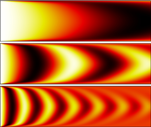
Figure 2. Field of periodic passive scalar fluctuation for  ${St}=0.5{\rm \pi}$ and
  ${St}=3{\rm \pi}$; The results in the first row are obtained analytically, using (4.1). The results in the second to fourth rows are obtained using FELiCS and are based on artificial diffusion,
  $D_{a}=0.001 D_{m}$, molecular diffusion,
  $D_{m}$, and the sum of molecular and turbulent diffusion,
  $D_{m}+D_{t}$, respectively.


The pattern seen in the respective plots of figure 2 resembles the plots based on large eddy simulation of a similar configuration conducted by Giusti et al. (Reference Giusti, Worth, Mastorakos and Dowling2017) (see figure 10 in Giusti et al. Reference Giusti, Worth, Mastorakos and Dowling2017). Furthermore, it explains the decrease observed in the gain of the TF: since the fluctuation in the passive scalar at the inlet is independent of  $y$, the integral of the scalar fluctuation in the
  $y$-direction is always equal to
  $2h\hat {c}_0$. At the outlet, however, the shear dispersion leads to regions which contribute positively and negatively to the integral. For very low frequencies, this effect is negligible. As frequency increases, however, it causes a decrease in gain of the TF, as illustrated in figure 3.
Despite its simplicity, the model of Giusti et al. (Reference Giusti, Worth, Mastorakos and Dowling2017) captures the attenuation of the TF gain at low frequencies very well. However, for higher frequencies, the drop in gain based on (4.1) is underestimated in comparison to the DNS results. For these frequencies, mean flow shear dispersion therefore appears to account for a part of the gain reduction only, which is in line with the conclusions of Giusti et al. (Reference Giusti, Worth, Mastorakos and Dowling2017).
The analytical results based on (4.1) allow for a validation of the linearized strategy for pure mean flow shear dispersion. While for these calculations the molecular and turbulent viscosities are set to zero, an artificial diffusion of  $D_{a}=0.001 \, D_{m}$ is applied. This is necessary to stabilize the numerical approach since pure mean flow shear dispersion leads to infinitely large gradients in the outer boundary layer towards the no-slip wall (see (4.1) and the respective plots in figure 2). The resulting field of passive scalar fluctuations is illustrated in figure 2 for
  ${St}=0.5{\rm \pi}$ and
  ${St}=2{\rm \pi}$. Although the artificial diffusion was chosen to be very small, it appears that, especially for high frequencies, the strong gradients in the outer boundary layer cause an annihilation of the
  $c$-fluctuation close to the wall. Nevertheless, this deviation from the analytical results does not impact the quality of the results in terms of the TF. This can be seen in figure 3, where the gains of the TF based on the linear approach using the artificial viscosity (red dashed line) and the analytical results (thin grey solid line) coincide.
4.2. Mean flow shear dispersion and molecular diffusion
In the next step, molecular diffusion is incorporated into the model, while turbulent mass transport is still neglected. Figure 3 shows the resulting gain of the TF (blue dash-dotted line). Accordingly, the impact of molecular diffusion is very small for low and intermediate frequencies. Only at high Strouhal numbers does the molecular diffusion appear to have a significant effect on the TF. The respective fields of periodic passive scalar fluctuations are shown for two different frequencies in the third row of figure 2. It explains the reduction in gain caused by molecular diffusion: since for small frequencies the characteristic wavelengths of the scalar fluctuation field are large, diffusion plays a minor role. For high frequencies, however, the characteristic length scale decreases and diffusion becomes more significant. This effect appears to be most pronounced in the boundary layer, where mean flow shear dispersion causes additional gradients in the  $y$-direction. A more thorough discussion on the effect of molecular diffusion on the overall convection is provided in § 4.4.
4.3. Mean flow shear dispersion, molecular and turbulent diffusion
In the final step, the effect of turbulent diffusion is no longer neglected and accounted for in the model using the eddy viscosity approach. The cross-streamwise distribution of eddy viscosity resulting from the two employed models (3.12) and (3.11) is shown in figure 4. Accordingly, both models result in very similar eddy viscosity profiles, which a posteriori justifies the application of the Cess model using the parameters given in § 3 in flows of significantly lower friction Reynolds numbers, as for example in Morra et al. (Reference Morra, Nogueira, Cavalieri and Henningson2021). In fact, all results of the linearized framework shown in this work only differ marginally between the two models. Since the Cess model only applies for the channel flow, while the model based on (3.12) can be applied to various configurations, only the results of the latter are shown in the following. Figure 4 furthermore shows the corresponding turbulent diffusivity as obtained from (3.10a,b).


Figure 2 compares the resulting  $\tilde {c}$ fields, i.e. with the contribution of
  $D_{t}$ in the fourth row, to the respective fields without turbulent contribution in the third row. In doing so, it allows for an intuitive explanation how turbulent diffusion contributes to the overall convection of the passive scalar fluctuation: while low frequencies are barely affected, the turbulent diffusion has a significant impact on the convection at high frequencies. This impact can be quantified by comparing the respective TFs to the DNS results, as seen in figure 3. The curves based on the DNS (black thick solid line) and the FELiCS results using a turbulent Prandtl number of
  ${Pr}_{t} = 0.9$ (green dashed line) show very good alignment, with minor deviations only for very low frequencies. These results demonstrate that the turbulence model is sufficiently accurate, and that turbulent diffusion makes a significant contribution to the overall convection of
  $\tilde {c}$.
The choice of the turbulent Prandtl number as  ${Pr}_{t}=0.9$ is arbitrary and based on empirical experience only. Therefore, a parametric study was conducted by varying the turbulent Prandtl number between
  $0.6$ and
  $1.2$. The range of the resulting TF gains are illustrated by the grey shaded area in figure 3. For low frequencies, the gain of the TFs of all turbulent Prandtl numbers coincide, as turbulent diffusion plays a subordinate role in this frequency range. For high frequencies, there is a noticeable but minor effect on the prediction when changing the Prandtl number. It therefore appears that the results of the linearized approach are robust with respect to the turbulent Prandtl number within the boundaries of the parametric study.
Displaying results in the time domain instead of the frequency domain often allows for a more intuitive, yet quantitative evaluation: figure 5 compares the IR of the previously investigated cases with the DNS data. While in the case of pure mean flow shear dispersion a distinct spike at a value of  $5.7$ clearly overestimates the DNS response, taking into account molecular and turbulent diffusion significantly improves the prediction of the DNS data. The IR including all relevant mechanisms still shows a slight deviation from the DNS response. This deviation can be explained by the difference in excitation signals applied in the DNS and the linearized approach. In the time-domain DNS, presumably for reasons of numerical stability, Morgans et al. (Reference Morgans, Goh and Dahan2013) applied a Gaussian profile in time instead of a sharp Dirac pulse. Therefore, the DNS response can only be an approximation to the true IR of the system. However, to obtain the response of the system to the Gaussian pulse, the IR based on FELiCS (green dashed line in figure 5) can be convolved with the Gaussian pulse in time domain. The result is illustrated in figure 6 for five streamwise positions. The plots show that the FELiCS results are congruent with the DNS results with minor deviations only for the response at
  $x_2=1.5h$, which underlines the accuracy of the present approach.

Figure 5. Comparison of IRs of various models to DNS data evaluated for  $x_2=6.0 h$.

Figure 6. Comparison of FELiCS results transferred to time domain with DNS data.
4.4. Quantification of the contribution of molecular and turbulent diffusive fluxes
In the analytical model based on (4.1) passive scalar transport was unidirectional in the  $x$-direction. Diffusion, however, as considered in §§ 4.2 and 4.3, causes transport of passive scalar fluctuations also in the
  $y$-direction. As a result, the channel half-height,
  $h$, constitutes a second characteristic length scale, which determines the significance of diffusive fluxes in the
  $y$-direction. Unlike in the model of Giusti et al. (Reference Giusti, Worth, Mastorakos and Dowling2017), changing the frequency therefore is not anymore equivalent to changing the measurement location,
  $x_2$. In contrast, the impact of diffusion on the transport depends on the frequency in a non-trivial way, which will be investigated in the following.
The linearized framework allows us to quantify the impact of molecular and turbulent diffusion in the configuration analysed via DNS by Morgans et al. in detail. The diffusion term in (3.14) is split into contributions from gradients in the  $x$- and
  $y$-direction as well as molecular and turbulent contributions, which are illustrated in figure 7 for four different frequencies. While the molecular flux in the
  $x$-direction is negligible, molecular diffusion in the
  $y$-direction is the predominant mechanism in the boundary layer. In the interior of the domain, however, turbulent diffusive fluxes are dominant. For low frequencies, it appears that turbulent fluxes in the
  $y$-direction (which only exist because of mean flow shear dispersion) are the dominant diffusive mechanism. With increasing frequency, however, the characteristic length scales of the diffusion in the
  $x$-direction and the respective time scales decrease. However, the time scales of diffusion in the
  $y$-direction are governed by the mean flow shear dispersion, which is a function of the mean flow profile and therefore constant. As a consequence, with increasing frequency, turbulent diffusion fluxes in the
  $x$-direction become more significant and finally are predominant for
  ${St} \geqslant 2.0{\rm \pi}$. In other words, for high frequencies, diffusive fluxes in the
  $x$-direction annihilate the periodic passive scalar fluctuations before mean flow shear dispersion allows for significant turbulent diffusion in the
  $y$-direction.

Figure 7. Diffusion term of (3.14) split into molecular and turbulent contributions in the  $x$- and
  $y$-directions.
5. Conclusion
The advection and diffusion of fuel ratio inhomogeneities and entropy waves in turbulent flows are investigated by means of a linearized mean field analysis. The governing equations are derived from a triple decomposition which separates the periodic passive scalar fluctuations from the mean and the stochastic turbulent field. The resulting transport equation for the periodic part is linearized and closed using an eddy viscosity model to account for the turbulent diffusion. The eddy viscosity field is determined from the Reynolds stresses and mean field gradients and constitutes, together with the temporal mean flow, the input to the linearized method. The validity of the closure model is motivated by the recent success in mean field stability analysis based on the momentum equations and is the core novelty of the current study.
The accuracy of the methodology is tested for a turbulent channel flow. The transport equation for the passive scalar is solved in frequency space in a two-dimensional domain using triangular finite elements. The mean velocity fields and Reynolds stresses are taken from DNS conducted in previous studies, which also provide the validation basis for our approach.
First, the solutions are sought for the case of zero diffusivity and compared to an analytic model. The observation of the resulting perturbation field reveals the mechanism that leads to the mean shear layer dispersion and corroborates previous analytic studies.
Next, the linearized methodology is applied to analyse the impact of the different mechanisms on the overall convection of the passive scalar. While for very low frequencies mean flow shear dispersion is the dominant mechanism, at higher frequencies diffusive processes need to be accounted for to reproduce the DNS results. Finally, an investigation of the diffusion term shows that, for the turbulent diffusion at medium frequencies, gradients in the cross-streamwise direction cause the strongest contribution. Whereas, for high frequencies, passive scalar gradients in the streamwise directions are the driving force for turbulent diffusion. Molecular diffusion, however, only has a minor effect on the overall convection of the passive scalar in the turbulent channel flow. Turbulence intensities in real world applications are significantly higher than in the canonical configurations that were so far investigated with analytical models or the method proposed in this study. As a consequence, the degree to which turbulence impacts the transport of entropy waves and fuel ratio inhomogeneities in a real engine can be expected to be more significant than in the turbulent channel flow under examination in this study.
Unlike the previously suggested low-order models, the framework presented in this study does not rely on any fitting of the IR to empirical data, but takes as input the statistics of the underlying flow. At the same time, the results are significantly more accurate, as demonstrated by the comparison with the DNS data.
The method comes with additional advantages. By including the linearized mass and momentum conservation equations, it can be extended in order to account for velocity fluctuations and variations in density. Furthermore, although the previous analytical models constitute valuable tools in the development process of gas turbines due to their low numerical cost, they cannot account for the non-parallelism of the flow and complicated geometries. In some cases, this can be a non-negligible source of error. The strategy of using unstructured finite elements in contrast, as is done in the proposed method, can be applied to these kinds of configurations.
Acknowledgements
The investigations were conducted as part of the joint research project ‘GREEN BELT – Dezentrale Gasturbinenanlagen für schnelle Reserven im Verbund mit erneuerbarer Energieumwandlung – Validierung der Technologien’.
Funding
The work was supported by the German Federal Ministry for Economic Affairs and Energy (BMWi) under grant number 0324314B. The authors gratefully acknowledge MAN Energy Solutions SE for their support and permission to publish this paper.
Declaration of interests
The authors report no conflict of interest.


