2. System dynamic analysis and modeling

The free-floating flexible-link and flexible-joints space manipulator system is composed of a rigid base ${{{B}}_0}$ , a rigid link ${{{B}}_1}$ , a flexible link ${{{B}}_2}$ , and two flexible joints ${{{O}}_i}({{i}} = 1,2)$ , as shown in Fig. 1. $\boldsymbol{OXY}$ is the inertial coordinate system, and ${{{O}}_{{j}}}{{{x}}_{{j}}}{{{y}}_{{j}}}$ is the main axis coordinate of ${{{B}}_{{j}}}\left( {{{j}} = 0,1,2} \right)$ . The centroids of ${{{B}}_0}$ , ${{{B}}_1}$ , and the system are ${{{O}}_{c0}}$ , ${{{O}}_{c1}}$ , and ${{C}}$ . Their position vectors are ${{\boldsymbol{r}}_0}$ , ${{\boldsymbol{r}}_1}$ , and ${{\boldsymbol{r}}_c}$ . The arbitrary point’s position vector on the flexible link ${{{B}}_2}$ is ${r_2}$ . ${{{q}}_{{j}}}$ is the motion angle of ${{{B}}_{{j}}}$ . ${{{\theta }}_{{i}}}$ is the motor rotor’s angle.

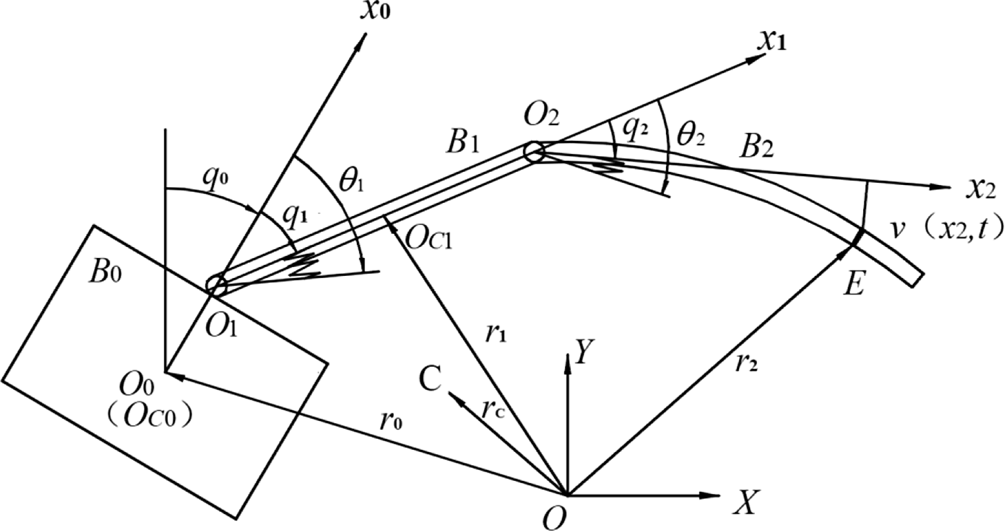
Figure 1. Free-floating flexible-link and flexible-joints space manipulator.

According to Spong’s assumption [Reference Spong57], we regard the flexible joints ${{{O}}_{{i}}}$ as a linear spring between the motor rotor and the link and the spring’s stiffness coefficient is $${k_{{\rm{\theta }}i}}$$ , as shown in Fig. 2. In this case, the rotor’s rotation angle ${{{\theta }}_{{i}}}$ will not always equal the link’s rotation angle ${{{q}}_{{i}}}$ . And, the flexible-joint error is: ${{{\sigma }}_{{i}}} = {{{\theta }}_{{i}}} - {{{q}}_{{i}}}$ .

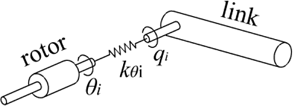
Figure 2. The simple model of flexible joint.

The flexible link ${{{B}}_2}$ is considered as an Euler–Bernoulli beam [Reference Krall58]. Neglecting the rotational inertia and shear deformation, based on the assumed mode method, the flexible link’s elastic deformation is:

(1) \begin{align}\upsilon ({{{x}}_2},{{t}}) = \sum\limits_{{{i}} = 1}^{{n}} {{\varphi _{{i}}}({{{x}}_2}){{{\delta }}_{{i}}}({{t}})} \end{align}

where ${\varphi t _{{i}}}({{{x}}_2})$ is the ${{i}}$ th mode function, ${{{\delta }}_{{i}}}({{t}})$ is the ${{i}}$ th mode coordinate, and ${{n}}$ is the retention mode number. Considering that the lower order modes play a leading role in elastic vibration and deformation, the first two lower-order modes can meet the accuracy requirements and reduce the calculation [Reference Guo, Jin, Chang and Wang59,Reference Lv, Wei and Chen60]. So, we choose ${{n}} = 2$ , that is, $\upsilon ({{{x}}_2},{{t}}) = {\varphi _1}({{{x}}_2}){{{\delta }}_1}({{t}}) + {\varphi _2}({{{x}}_2}){{{\delta }}_2}({{t}})$ .

According to the geometric position relationship

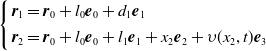(2) \begin{align}\left\{ \begin{array}{l} {{{\boldsymbol{r}}_1} = {{\boldsymbol{r}}_0} + {{{l}}_0}{{\boldsymbol{e}}_0} + {{{d}}_1}{{\boldsymbol{e}}_1}} \\[4pt] {{{\boldsymbol{r}}_2} = {{\boldsymbol{r}}_0} + {{{l}}_0}{{\boldsymbol{e}}_0} + {{{l}}_1}{{\boldsymbol{e}}_1} + {{{x}}_2}{{\boldsymbol{e}}_2} + \upsilon ({{{x}}_2},{{t}}){{\boldsymbol{e}}_3}} \end{array}\right.\end{align}

where ${{{l}}_0}$ is the distance between ${{{O}}_{c0}}$ and ${{{O}}_1}$ , ${{{d}}_1}$ is the distance between ${{{O}}_1}$ and ${{{O}}_{c1}}$ , ${{{l}}_1}$ is the length of ${{{B}}_1}$ .

${e_0} = {\left[ \begin{array}{c} {\sin ({{{q}}_0})} \\[4pt] {\cos ({{{q}}_0})} \end{array}\right]^{\rm T}}$ , ${e_1} = {\left[ {\begin{array}{c}{\sin ({{{q}}_0} + {{{q}}_1})}\\[4pt]{\cos ({{{q}}_0} + {{{q}}_1})}\end{array}} \right]^{\rm T}}$ , ${e_2} = {\left[ {\begin{array}{c}{\sin ({{{q}}_0} + {{{q}}_1} + {{{q}}_2})}\\[4pt]{\cos ({{{q}}_0} + {{{q}}_1} + {{{q}}_2})}\end{array}} \right]^{\rm T}}$ , ${e_3} = {\left[ \begin{array}{c} {\cos ({{{q}}_0} + {{{q}}_1} + {{{q}}_2})} \\[4pt] { - \sin ({{{q}}_0} + {{{q}}_1} + {{{q}}_2})} \end{array} \right]^{\rm T}}$ .

The system’s total center theorem of mass is:

(3) \begin{align}{{{m}}_0}{{\boldsymbol{r}}_0} + {{{m}}_1}{{\boldsymbol{r}}_1} + {{\rho }}\int_0^{{l_2}} {{{\boldsymbol{r}}_2}} {\rm d}{{{x}}_2} = {{M}}{{\boldsymbol{r}}_c}\end{align}

where ${{{m}}_0}$ is the mass of ${{{B}}_0}$ , ${{{m}}_1}$ is the mass of ${{{B}}_1}$ , ${{\rho }}$ is the linear density of ${{{B}}_2}$ , and ${{{l}}_2}$ is the length of ${{{B}}_2}$ . ${{M}}$ is the total system’s mass, ${{M}} = {{{m}}_0} + {{{m}}_1} + {{\rho }}{{{l}}_2}$ . The mass of the motor is negligible.

The position vectors can be expressed as follows:

(4) \begin{align}{{\boldsymbol{r}}_{{i}}} = {{\boldsymbol{r}}_c} + {{{R}}_{{{i}}0}}{{\boldsymbol{e}}_0} + {{{R}}_{{{i}}1}}{{\boldsymbol{e}}_1} + {{{R}}_{{{i}}2}}{{\boldsymbol{e}}_2} + ({{{R}}_{{{i}}3}}{{{\delta }}_1} + {{{R}}_{{{i}}4}}{{{\delta }}_2}){{\boldsymbol{e}}_3}\end{align}

where ${{{R}}_{00}} = - ({{{m}}_1} + {{\rho }}{{{l}}_2}){{{l}}_0}/{{M}}$ , ${{{R}}_{01}} = - ({{{m}}_1}{{{d}}_1} + {{\rho }}{{{l}}_2}{{{l}}_1})/{{M}}$ , ${{{R}}_{02}} = - {{\rho l}}_2^2/(2{{M}})$ , ${{{R}}_{03}} = - {{\rho }}\int_0^{{{{l}}_2}} {{\varphi _1}({{{x}}_2})} d{{{x}}_2}/{{M}}$ , ${{{R}}_{04}} = - {{\rho }}\int_0^{{{{l}}_2}} {{\varphi _2}({{{x}}_2})} d{{{x}}_2}/{{M}}$ , ${{{R}}_{10}} = {{{R}}_{00}} + {{{l}}_0}$ , ${{{R}}_{11}} = {{{R}}_{01}} + {{{d}}_1}$ , ${{{R}}_{12}} = {{{R}}_{02}}$ , ${{{R}}_{13}} = {{{R}}_{03}}$ , ${{{R}}_{14}} = {{{R}}_{04}}$ , ${{{R}}_{20}} = {{{R}}_{00}} + {{{l}}_0}$ , ${{{R}}_{21}} = {{{R}}_{01}} + {{{l}}_1}$ , ${{{R}}_{22}} = {{{R}}_{02}} + {{{x}}_2}$ , ${{{R}}_{23}} = {{{R}}_{03}} + {\varphi _1}({{{x}}_2})$ , ${{{R}}_{24}} = {{{R}}_{04}} + {\varphi _2}({{{x}}_2})$ .

Differentiating Eq. (4), we have:

(5) \begin{align}{\dot{{\boldsymbol{r}}}_{{i}}} = {\dot{{\boldsymbol{r}}}_c} + {{{R}}_{{{i}}0}}{\dot{{\boldsymbol{e}}}_0} + {{{R}}_{{{i}}1}}{\dot{{\boldsymbol{e}}}_1} + {{{R}}_{{{i}}2}}{\dot{e}_2} + ({{{R}}_{{{i}}3}}{{{\delta }}_1} + {{{R}}_{{{i}}4}}{{{\delta }}_2}){\dot{{\boldsymbol{e}}}_3} + ({{{R}}_{{{i}}3}}{{{\dot{\delta} }}_1} + {{{R}}_{{{i}}4}}{{{\dot{\delta} }}_2}){{\boldsymbol{e}}_3}\end{align}

where ${\dot{{\boldsymbol{r}}}_{{i}}}$ , ${\dot{{\boldsymbol{r}}}_c}$ , ${{{\dot{\delta} }}_1}$ , and ${{{\dot{\delta} }}_2}$ are the first derivative of ${{\boldsymbol{r}}_{{i}}}$ , ${{\boldsymbol{r}}_c}$ , ${{{\delta }}_1}$ , and ${{{\delta }}_2}$ . ${\dot{{\boldsymbol{e}}}_0} = {{\dot{{q}}}_0}{\left[ {\begin{array}{c}{\cos ({{{q}}_0})}\\[4pt]{ - \sin ({{{q}}_0})}\end{array}} \right]^{\rm T}}$ , ${\dot{{\boldsymbol{e}}}_1} = ({{\dot{{q}}}_0} + {{\dot{{q}}}_1}){\left[ {\begin{array}{c}{\cos ({{{q}}_0} + {{{q}}_1})}\\[4pt]{ - \sin ({{{q}}_0} + {{{q}}_1})}\end{array}} \right]^{\rm T}}$ , ${\dot{{\boldsymbol{e}}}_2} = ({{\dot{{q}}}_0} + {{\dot{{q}}}_1} + {{\dot{{q}}}_2}){\left[ {\begin{array}{c}{\cos ({{{q}}_0} + {{{q}}_1} + {{{q}}_2})}\\[4pt]{ - \sin ({{{q}}_0} + {{{q}}_1} + {{{q}}_2})}\end{array}} \right]^{\rm T}}$ , and ${\dot{{\boldsymbol{e}}}_3} = ({{\dot{{q}}}_0} + {{\dot{{q}}}_1} + {{\dot{{q}}}_2}){\left[ {\begin{array}{c}{ - \sin ({{{q}}_0} + {{{q}}_1} + {{{q}}_2})}\\[4pt]{ - \cos ({{{q}}_0} + {{{q}}_1} + {{{q}}_2})}\end{array}} \right]^{\rm T}}$ .

Without loss of generality, the system satisfies the momentum conservation and the angular momentum conservation. Let the initial values of the momentum and the angular momentum be zero, the system’s momentum conservation equation and the angular momentum conservation equation can be expressed as:

(6) \begin{align}{{{m}}_0}{\dot{{\boldsymbol{r}}}_0} + {{{m}}_1}{\dot{{\boldsymbol{r}}}_1} + {{\rho }}\int_0^{{{{l}}_2}} {{{\dot{{\boldsymbol{r}}}}_2}} {\rm d}{{{x}}_2} = 0\end{align}

(7) \begin{align}({{{m}}_0}{{\boldsymbol{r}}_0} \times {\dot{{\boldsymbol{r}}}_0} + {{{J}}_0}{\omega _0}) + ({{{m}}_1}{{\boldsymbol{r}}_1} \times {\dot{{\boldsymbol{r}}}_1} + {{{J}}_1}{\omega _1}) + {{\rho }}\int_0^{{{{l}}_2}} {({{\boldsymbol{r}}_2} \times {{\dot{{\boldsymbol{r}}}}_2})} {\rm d}{{{x}}_2} + \sum\limits_{{{i}} = 1}^2 {({{{J}}_{\rm{\theta } {{i}}}}{\omega _{\rm{\theta } {{i}}}})} = 0\end{align}

where ${{{J}}_0}$ is the inertial moment of ${{{B}}_0}$ , ${{{J}}_1}$ is the inertial moment of ${{{B}}_1}$ , and ${{{J}}_{\rm{\theta } {{i}}}}$ is the inertial moment of the motor rotor. ${\omega _0}$ is the angular velocity of ${{{B}}_0}$ , ${{{\omega }}_0} = {{\dot{{q}}}_0}$ . ${\omega _1}$ is the angular velocity of ${{{B}}_1}$ , ${{{\omega }}_1} = ({{\dot{{q}}}_0} + {{\dot{{q}}}_1})$ . ${\omega _{\rm{\theta } {{i}}}}$ is the angular velocity of motor rotor, ${{{\omega }}_{\rm{\theta } {{i}}}} = {{{\dot{\theta} }}_{{i}}}$ .

The system’s kinetic energy ${{T}}$ contains the manipulator system’s kinetic energy ${{{T}}_r}$ and the motor rotors’ kinetic energy ${T_\rm{\theta } }$ :

(8) \begin{align}{{T}} = {{{T}}_r} + {{{T}}_\rm{\theta } }\end{align}

where ${{{T}}_r} = {{{T}}_0} + {{{T}}_1} + {{{T}}_2}$ , ${{{T}}_\rm{\theta } } = {{{T}}_{\rm{\theta } 1}} + {{{T}}_{\rm{\theta } 2}}$ . ${{{T}}_0} = \frac{1}{2}{{{m}}_0}\dot{{\boldsymbol{r}}}_0^2 + \frac{1}{2}{{{J}}_0}{{\omega }}_0^2$ is ${{{B}}_0}$ ’s kinetic energy, ${{{T}}_1} = \frac{1}{2}{{{m}}_1}\dot{{\boldsymbol{r}}}_1^2 + \frac{1}{2}{{{J}}_1}{{\omega }}_1^2$ is ${{{B}}_1}$ ’s kinetic energy, ${{{T}}_2} = \frac{1}{2}{{\rho }}\int_0^{{{{l}}_2}} {\dot{{\boldsymbol{r}}}_2^2} {\rm d}{{\boldsymbol{x}}_2}$ is ${{{B}}_2}$ ’s kinetic energy, ${{{T}}_{\rm{\theta } {{i}}}} = \frac{1}{2}{{{J}}_{\rm{\theta } {{i}}}}{{\omega }}_{\rm{\theta } {{i}}}^2$ is the motor rotor’s kinetic energy.

Neglecting the gravity in the space. The system’s potential energy ${{U}}$ contains the flexible link’s bending strain energy ${{{U}}_r}$ and the flexible joints’ elastic deformation potential energy ${{{U}}_\rm{\theta } }$ :

(9) \begin{align}{{U}} = {{{U}}_r} + {{{U}}_\rm{\theta } }\end{align}

where ${{{U}}_r} = \frac{1}{2}{{EI}}{\int_0^{{{{l}}_2}} {\left( {\frac{{{\partial ^2}\upsilon ({{{x}}_2},{{t}})}}{{\partial {{x}}_2^2}}} \right)} ^2}{\rm d}{{{x}}_2}$ , ${{{U}}_\rm{\theta } } = \frac{1}{2}\sum\limits_{{{i}} = 1}^2 {{{{k}}_{\rm{\theta } {{i}}}}{{({{{\theta }}_{{i}}}{{ - }}{{{q}}_{{i}}})}^2}} $ , ${{EI}}$ is the bending stiffness of ${{{B}}_2}$ .

The system’s Lagrangian function is: ${{L}} = {{T}} - {{U}}$ . Choose $${\boldsymbol{Q}} = {\left[ {\matrix{ {{\theta _1}\quad {\theta _2}\quad {q_0}\quad {q_1}\quad {q_2}\quad {\delta _1}\quad {\delta _2}} \cr } } \right]^{\rm{T}}}$$ as the system’s generalized coordinate, $${\boldsymbol{F}} = {\left[ {\matrix{ {{\tau _1}\quad {\tau _2}\quad 0\quad 0\quad 0\quad 0\quad 0} \cr } } \right]^{\rm{T}}}$$ as the generalized force. Then, according to Lagrange’s second type equation $\frac{\rm d}{{\rm d{{t}}}}\left( {\frac{{\partial {{L}}}}{{\partial \dot{{\boldsymbol{Q}}}}}} \right) - \frac{{\partial {{L}}}}{{\partial {{\boldsymbol{Q}}}}} = {\boldsymbol{F}}$ , the system’s dynamic equation has the following form

(10a) \begin{align}{{\boldsymbol{J}}_{\rm{\theta }} }\ddot{\boldsymbol\theta} + {{\boldsymbol{K}}_{\rm{\theta }}}(\boldsymbol\theta - {{\boldsymbol{q}}_\rm{\theta } }) = \boldsymbol\tau + {\boldsymbol\tau _{\text{d}}}\end{align}

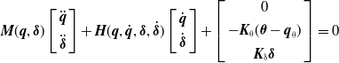(10b) \begin{align}{\boldsymbol{M}}({\boldsymbol{q}},\boldsymbol\delta )\left[ {\begin{array}{c}{\ddot{{\boldsymbol{q}}}}\\[6pt]{\ddot{\boldsymbol\delta} }\end{array}} \right] + {\boldsymbol{H}}({\boldsymbol{q}},\dot{{\boldsymbol{q}}},\boldsymbol\delta ,\dot{\boldsymbol\delta} )\left[ {\begin{array}{c}{\dot{{\boldsymbol{q}}}}\\[4pt]{\dot{\boldsymbol\delta} }\end{array}} \right] + \left[ {\begin{array}{c}0\\[4pt]{ - {{\boldsymbol{K}}_\rm{\theta } }(\boldsymbol\theta - {{\boldsymbol{q}}_\rm{\theta } })}\\[4pt]{{{\boldsymbol{K}}_{{\delta }} }\boldsymbol\delta }\end{array}} \right] = 0\end{align}

where $${\boldsymbol{\theta }} = {[\matrix{ {{\theta _1}\quad {\theta _2}} \cr } ]^{\rm{T}}}$$ , $${{\boldsymbol{q}}_\theta } = {[\matrix{ {{q_1}\quad {q_2}} \cr } ]^{\rm{T}}}$$ , $${\boldsymbol{q}} = {[\matrix{ {{q_0}\quad {q_1}\quad {q_2}} \cr } ]^{\rm{T}}}$$ , $${\boldsymbol{\delta }} = {[\matrix{ {{\delta _1}\quad {\delta _2}} \cr } ]^{\rm{T}}}$$ , ${{\boldsymbol{J}}_\rm{\theta } } = {\rm{diag}}({{{J}}_{\rm{\theta } 1}},{{{J}}_{\rm{\theta } 2}}) \in {{\boldsymbol{R}}^{2 \times 2}}$ is the diagonal and positive definite inertia matrix of the motor, ${{\boldsymbol{K}}_\rm{\theta } } = {\rm{diag}}({{{k}}_{\rm{\theta } 1}},{{{k}}_{\rm{\theta } 2}}) \in {{\boldsymbol{R}}^{2 \times 2}}$ is the simplified linear spring stiffness coefficient matrix of flexible joint, ${\boldsymbol{M}}({\boldsymbol{q}},\boldsymbol\delta ) \in {{\boldsymbol{R}}^{5 \times 5}}$ is the space manipulator’s symmetric positive definite inertia matrix, ${\boldsymbol{H}}({\boldsymbol{q}},\dot{{\boldsymbol{q}}},\boldsymbol\delta ,\dot{\boldsymbol\delta} )\left[ {\begin{array}{c}{\dot{{\boldsymbol{q}}}}\\[4pt]{\dot{\boldsymbol\delta} }\end{array}} \right] \in {{\boldsymbol{R}}^{5 \times 1}}$ is a column vector containing the Coriolis force and centrifugal force, ${{\boldsymbol{K}}_{ {\delta }} } = {\rm{diag}}({{{k}}_{ {\delta } 1}},{{{k}}_{ {\delta } 2}})$ is the flexible link’s stiffness coefficient matrix, ${{{k}}_{ {\delta } {{i}}}} = \int_0^{{{{l}}_2}} {{{EI}}{\varphi^{\prime\prime}_{{i}}}^{\rm T}} \varphi^{\prime\prime}_{{i}}{\rm d}{{{x}}_2}$ . $${\boldsymbol{\tau }} = {[\matrix{ {{\tau _1}\quad {\tau _2}} \cr } ]^{\rm{T}}} \in {{\boldsymbol{R}}^{2 \times 1}}$$ is the output torque of the motors, and ${\boldsymbol\tau _{\rm d}} \in {{\boldsymbol{R}}^{2 \times 1}}$ is the external interference torque.

It can be seen that Eq. (10a) is the dynamic equation of the motor and Eq. (10b) is the dynamic equation of the space manipulator.

3. Singular perturbation decomposition and control design

The free-floating flexible-link and flexible-joints space manipulator system is a rigid-flexible coupling system. The interaction between the rigid variables and the flexible variables will make the controller’s design difficult and affect the control quality. To reduce the interaction between variables, we use the singular perturbation method to decompose the complex system into a slow subsystem and a fast subsystem with independent time scales. The slow subsystem describes the system’s rigid movement. The fast subsystem describes the system’s flexible movement. Then, the appropriate controller is designed for each subsystem. The slow subsystem’s controller ${\boldsymbol\tau _{\rm s}}$ is designed to achieve the desired trajectory asymptotic tracking. The fast subsystem’s controller ${\boldsymbol\tau _{\rm f}}$ is designed to suppress the double vibration caused by the flexible joints and the flexible link [Reference Spong61]. So, we can write the system’s total controller as: $\boldsymbol\tau = {\boldsymbol\tau _{\rm s}} + {\boldsymbol\tau _{\rm f}}$ .

First, we decomposed Eq. (10b) into the following form:

(11) $$\left[ {\matrix{ {{{\boldsymbol{M}}_{11}}} & {{{\boldsymbol{M}}_{12}}} & {{{\boldsymbol{M}}_{13}}} \cr {{{\boldsymbol{M}}_{21}}} & {{{\boldsymbol{M}}_{22}}} & {{{\boldsymbol{M}}_{23}}} \cr {{{\boldsymbol{M}}_{31}}} & {{{\boldsymbol{M}}_{32}}} & {{{\boldsymbol{M}}_{33}}} \cr } } \right] \cdot \left[ {\matrix{ {{{\mathop {\boldsymbol{q}}\limits^{..} }_0}} \cr {{{\mathop {\boldsymbol{q}}\limits^{..} }_\theta }} \cr {\mathop {\boldsymbol{\delta }}\limits^{..} } \cr } } \right] + \left[ {\matrix{ {{{\boldsymbol{N}}_1}} \cr {{{\boldsymbol{N}}_2}} \cr {{{\boldsymbol{N}}_3}} \cr } } \right] + \left[ {\matrix{ 0 \cr { - {{\boldsymbol{K}}_\theta }({\boldsymbol{\theta }} - {{\boldsymbol{q}}_\theta })} \cr {{{\boldsymbol{K}}_\delta }{\boldsymbol{\delta }}} \cr } } \right] = 0$$

where ${{\boldsymbol{M}}_{11}} \in {{\boldsymbol{R}}^{1 \times 1}}$ , ${{\boldsymbol{M}}_{12}} \in {{\boldsymbol{R}}^{1 \times 2}}$ , ${{\boldsymbol{M}}_{13}} \in {{\boldsymbol{R}}^{1 \times 2}}$ , ${{\boldsymbol{M}}_{21}} \in {{\boldsymbol{R}}^{2 \times 1}}$ , ${{\boldsymbol{M}}_{22}} \in {{\boldsymbol{R}}^{2 \times 2}}$ , ${{\boldsymbol{M}}_{23}} \in {{\boldsymbol{R}}^{2 \times 2}}$ , ${{\boldsymbol{M}}_{31}} \in {{\boldsymbol{R}}^{2 \times 1}}$ , ${{\boldsymbol{M}}_{32}} \in {{\boldsymbol{R}}^{2 \times 2}}$ , and ${{\boldsymbol{M}}_{33}} \in {{\boldsymbol{R}}^{2 \times 2}}$ are the sub-matrices of ${\boldsymbol{M}}({\boldsymbol{q}},\boldsymbol\delta )$ . ${{\boldsymbol{N}}_1} \in {{\boldsymbol{R}}^{1 \times 1}}$ , ${{\boldsymbol{N}}_2} \in {{\boldsymbol{R}}^{2 \times 1}}$ , ${{\boldsymbol{N}}_3} \in {{\boldsymbol{R}}^{2 \times 1}}$ are the sub-matrices of ${\boldsymbol{H}}({\boldsymbol{q}},\dot{{\boldsymbol{q}}},\boldsymbol{\delta} ,\dot{\boldsymbol\delta} )\left[ {\begin{array}{c}{\dot{{\boldsymbol{q}}}}\\[4pt]{\dot{\boldsymbol\delta} }\end{array}} \right]$ .

From Eq. (11), we have

(12) \begin{align}{{{\ddot{ q}}}_0} = - {\boldsymbol{M}}_{11}^{ - 1}({{\boldsymbol{M}}_{12}}{\ddot{{\boldsymbol{q}}}_\rm{\theta } } + {{\boldsymbol{M}}_{13}}\ddot{\boldsymbol\delta} ) - {\boldsymbol{M}}_{11}^{ - 1}{{\boldsymbol{N}}_1}\end{align}

Substitute Eq. (12) into Eq. (11), we have

(13) $$\left[ {\matrix{ {{{\boldsymbol{D}}_{11}}} & {{{\boldsymbol{D}}_{12}}} \cr {{{\boldsymbol{D}}_{21}}} & {{{\boldsymbol{D}}_{22}}} \cr } } \right] \cdot \left[ {\matrix{ {{{\mathop {\boldsymbol{q}}\limits^{..} }_\theta }} \cr {\mathop {\boldsymbol{\delta }}\limits^{..} } \cr } } \right] + \left[ {\matrix{ {{{\boldsymbol{C}}_1}} \cr {{{\boldsymbol{C}}_2}} \cr } } \right] + \left[ {\matrix{ { - {{\boldsymbol{K}}_\theta }({\boldsymbol{\theta }} - {{\boldsymbol{q}}_\theta })} \cr {{{\boldsymbol{K}}_\delta }{\boldsymbol{\delta }}} \cr } } \right] = 0$$

where ${{\boldsymbol{D}}_{11}} = - {{\boldsymbol{M}}_{21}}{\boldsymbol{M}}_{11}^{ - 1}{{{\boldsymbol{M}}}_{12}} + {{{\boldsymbol{M}}}_{22}}$ , ${{{\boldsymbol{D}}}_{12}} = - {{{\boldsymbol{M}}}_{21}}{{\boldsymbol{M}}}_{11}^{ - 1}{{{\boldsymbol{M}}}_{13}} + {{{\boldsymbol{M}}}_{23}}$ , ${{{\boldsymbol{D}}}_{21}} = - {{{\boldsymbol{M}}}_{31}}{{\boldsymbol{M}}}_{11}^{ - 1}{{{\boldsymbol{M}}}_{12}} + {{{\boldsymbol{M}}}_{32}}$ , ${{{\boldsymbol{D}}}_{22}} = - {{{\boldsymbol{M}}}_{31}}{{\boldsymbol{M}}}_{11}^{ - 1}{{{\boldsymbol{M}}}_{13}} + {{{\boldsymbol{M}}}_{33}}$ , ${{{\boldsymbol{C}}}_1} = - {{{\boldsymbol{M}}}_{21}}{{\boldsymbol{M}}}_{11}^{ - 1}{{{\boldsymbol{N}}}_1} + {{{\boldsymbol{N}}}_2}$ , ${{{\boldsymbol{C}}}_2} = - {{{\boldsymbol{M}}}_{31}}{{\boldsymbol{M}}}_{11}^{ - 1}{{{\boldsymbol{N}}}_1} + {{{\boldsymbol{N}}}_3}$ .

Because the matrix $$\left[ {\matrix{ {{{\boldsymbol{D}}_{11}}} & {{{\boldsymbol{D}}_{12}}} \cr {{{\boldsymbol{D}}_{21}}} & {{{\boldsymbol{D}}_{22}}} \cr } } \right]$$ is symmetric and positive definite, it is reversible. Its inverse matrix can be expressed as:

(14) $${\left[ {\matrix{ {{{\boldsymbol{D}}_{11}}} & {{{\boldsymbol{D}}_{12}}} \cr {{{\boldsymbol{D}}_{21}}} & {{{\boldsymbol{D}}_{22}}} \cr } } \right]^{ - 1}} = \left[ {\matrix{ {{{\boldsymbol{G}}_{11}}} & {{{\boldsymbol{G}}_{12}}} \cr {{{\boldsymbol{G}}_{21}}} & {{{\boldsymbol{G}}_{22}}} \cr } } \right]$$

Let the flexible-joint error vector $${\boldsymbol{\sigma }} = {\boldsymbol{\theta }} - {{\boldsymbol{q}}_\theta } = {[\matrix{ {{\sigma _1}\quad {\sigma _2}} \cr } ]^{\rm{T}}}$$ . We rewrite Eqs. (10) and (13) as following

(15a) \begin{align}\ddot{\boldsymbol\sigma} = \ddot{\boldsymbol\theta} - {\ddot{{{\boldsymbol{q}}}}_\rm{\theta } } = - {{\boldsymbol{J}}}_\rm{\theta } ^{ - 1}{{{\boldsymbol{K}}}_\rm{\theta } }\sigma + {{\boldsymbol{J}}}_\rm{\theta } ^{ - 1}(\boldsymbol\tau + {\boldsymbol\tau _{\rm d}}) - {\ddot{{\boldsymbol{q}}}_\rm{\theta } }\end{align}

(15b) \begin{align}{\ddot{{\boldsymbol{q}}}_\rm{\theta } } = - {{\boldsymbol{G}}_{11}}{{\boldsymbol{C}}_1} - {{\boldsymbol{G}}_{12}}{{\boldsymbol{C}}_2} - {{\boldsymbol{G}}_{12}}{{\boldsymbol{K}}_{ {\delta }} }\boldsymbol\delta + {{\boldsymbol{G}}_{11}}{{\boldsymbol{K}}_\rm{\theta } }\boldsymbol\sigma \end{align}

(15c) \begin{align}\ddot{\boldsymbol\delta} = - {{\boldsymbol{G}}_{21}}{{\boldsymbol{C}}_1} - {{\boldsymbol{G}}_{22}}{{\boldsymbol{C}}_2} - {\boldsymbol{G}}{}_{22}{{\boldsymbol{K}}_{ {\delta }} }\boldsymbol\delta + {{\boldsymbol{G}}_{21}}{{\boldsymbol{K}}_\rm{\theta } }\boldsymbol\sigma \end{align}

Defining a singular perturbation factor: ${{{\varepsilon }}^2} = 1/\min \left\{ {{{{k}}_{ {\delta } 1}},{{{k}}_{ {\delta } 2}},{{{k}}_{\rm{\theta } 1}}, {{{k}}_{\rm{\theta } 2}}} \right\}$ , two variables: ${{\boldsymbol{z}}_{ {\delta }} } = \boldsymbol\delta /{{{\varepsilon }}^2}$ and ${{\boldsymbol{z}}_\rm{\theta } } = \boldsymbol\sigma /{{{\varepsilon }}^2}$ , two matrices: ${{\boldsymbol{K}}_{ {\delta } \varepsilon }} = {{{\varepsilon }}^2}{{\boldsymbol{K}}_{ {\delta }} }$ and ${{\boldsymbol{K}}_{\rm{\theta } \varepsilon }} = {{{\varepsilon }}^2}{{\boldsymbol{K}}_\rm{\theta } }$ . Then, the singular perturbation model of the system’s dynamic equation is established:

(16a) \begin{align}{{\rm{\varepsilon }}^2}{\ddot{{\boldsymbol{z}}}_\rm{\theta } } = - {\boldsymbol{J}}_\rm{\theta } ^{ - 1}{{\boldsymbol{K}}_{\rm{\theta } \varepsilon }}{{\boldsymbol{z}}_\rm{\theta } } + {\boldsymbol{J}}_\rm{\theta } ^{ - 1}\left( {\boldsymbol\tau + {\boldsymbol\tau _{\rm d}}} \right) - {\ddot{{\boldsymbol{q}}}_\rm{\theta } }\end{align}

(16b) \begin{align}{\ddot{{\boldsymbol{q}}}_\rm{\theta } } = - {{\boldsymbol{G}}_{11}}{{\boldsymbol{C}}_1} - {{\boldsymbol{G}}_{12}}{{\boldsymbol{C}}_2} - {{\boldsymbol{G}}_{12}}{{\boldsymbol{K}}_{ {\delta } \varepsilon }}{{\boldsymbol{z}}_{ {\delta }} } + {{\boldsymbol{G}}_{11}}{{\boldsymbol{K}}_{\rm{\theta } \varepsilon }}{{\boldsymbol{z}}_\rm{\theta } }\end{align}

(16c) \begin{align}{{\rm{\varepsilon }}^2}{\ddot{{\boldsymbol{z}}}_{ {\delta }} } = - {{\boldsymbol{G}}_{21}}{{\boldsymbol{C}}_1} - {{\boldsymbol{G}}_{22}}{{\boldsymbol{C}}_2} - {\boldsymbol{G}}{}_{22}{{\boldsymbol{K}}_{ {\delta } \varepsilon }}{{\boldsymbol{z}}_{ {\delta }} } + {{\boldsymbol{G}}_{21}}{{\boldsymbol{K}}_{\rm{\theta } \varepsilon }}{{\boldsymbol{z}}_\rm{\theta } }\end{align}

3.1. The slow subsystem

The slow subsystem only describes the system’s rigid movement. So here, we can ignore the influences of the flexible joints and the flexible link. Let ${\rm{\varepsilon }} = 0$ , then Eq. (16) can be rewritten as:

(17a) \begin{align}0 = - {\boldsymbol{J}}_\rm{\theta } ^{ - 1}{\bar{{\boldsymbol{K}}}_{\rm{\theta } \varepsilon }}{\bar{{\boldsymbol{z}}}_\rm{\theta } } + {\boldsymbol{J}}_\rm{\theta } ^{ - 1}\left( {{\boldsymbol\tau _{\rm s}} + {\boldsymbol\tau _{\rm d}}} \right) - {\ddot{{\boldsymbol{q}}}_\rm{\theta } }\end{align}

(17b) \begin{align}{\ddot{{\boldsymbol{q}}}_\rm{\theta } } = - {\bar{{\boldsymbol{G}}}_{11}}{\bar{C}_1} - {\bar{{\boldsymbol{G}}}_{12}}{\bar{C}_2} - {\bar{{\boldsymbol{G}}}_{12}}{\bar{{\boldsymbol{K}}}_{ {\delta } \varepsilon }}{\bar{{\boldsymbol{z}}}_{ {\delta }} } + {\bar{{\boldsymbol{G}}}_{11}}{\bar{{\boldsymbol{K}}}_{\rm{\theta } \varepsilon }}{\bar{{\boldsymbol{z}}}_\rm{\theta } }\end{align}

(17c) \begin{align}0 = - {\bar{{\boldsymbol{G}}}_{21}}{\bar{C}_1} - {\bar{{\boldsymbol{G}}}_{22}}{\bar{C}_2} - \bar{{\boldsymbol{G}}}{}_{22}{\bar{{\boldsymbol{K}}}_{ {\delta } \varepsilon }}{\bar{{\boldsymbol{z}}}_{ {\delta }} } + {\bar{{\boldsymbol{G}}}_{21}}{\bar{{\boldsymbol{K}}}_{\rm{\theta } \varepsilon }}{\bar{{\boldsymbol{z}}}_\rm{\theta } }\end{align}

where $\bar{{\boldsymbol{A}}}$ is the corresponding matrix or variable of ${\boldsymbol{A}}$ when ${\rm{\varepsilon }} = 0$ , that is, the corresponding matrix or variable calculated in the slowly varying time scale.

From Eq. (17a)

(18) \begin{align}{\bar{{\boldsymbol{z}}}_\rm{\theta } } = \bar{{\boldsymbol{K}}}_{\rm{\theta } \varepsilon }^{ - 1}({\boldsymbol\tau _{\rm s}} + {\boldsymbol\tau _{\rm d}} - {{\boldsymbol{J}}_\rm{\theta } }{\ddot{{\boldsymbol{q}}}_\rm{\theta } })\end{align}

Substituting Eq. (18) into Eq. (17c), we can get:

(19) \begin{align}{\bar{{\boldsymbol{z}}}_{ {\delta }} } = \bar{{\boldsymbol{K}}}_{ {\delta } \varepsilon }^{ - 1}\bar{{\boldsymbol{G}}}_{22}^{ - 1}[ - {\bar{{\boldsymbol{G}}}_{21}}{\bar{{\boldsymbol{C}}}_1} - {\bar{{\boldsymbol{G}}}_{22}}{\bar{{\boldsymbol{C}}}_2} + {\bar{{\boldsymbol{G}}}_{21}}({\boldsymbol\tau _{\rm s}} + {\boldsymbol\tau _{\rm d}} - {{\boldsymbol{J}}_\rm{\theta } }{\ddot{{\boldsymbol{q}}}_\rm{\theta } })]\end{align}

Then, substituting Eqs. (18) and (19) into Eq. (17b), the slow subsystem’s dynamics equation can be obtained as:

(20) \begin{align}{{\boldsymbol{D}}_{\rm s}}{\ddot{{\boldsymbol{q}}}_\rm{\theta } } + {{\boldsymbol{C}}_{\rm s}} = {\boldsymbol\tau _{\rm s}} + {\boldsymbol\tau _{\rm d}}\end{align}

where ${{\boldsymbol{D}}_{\rm s}} = {[{\bar{{\boldsymbol{G}}}_{11}} - {\bar{{\boldsymbol{G}}}_{12}}\bar{{\boldsymbol{G}}}_{22}^{ - 1}{\bar{{\boldsymbol{G}}}_{21}}]^{ - 1}} + {J_\rm{\theta } }$ , ${{\boldsymbol{C}}_{\rm s}} = {[{\bar{{\boldsymbol{G}}}_{11}} - {\bar{{\boldsymbol{G}}}_{12}}\bar{{\boldsymbol{G}}}_{22}^{ - 1}{\bar{{\boldsymbol{G}}}_{21}}]^{ - 1}}({\bar{{\boldsymbol{G}}}_{11}} - {\bar{{\boldsymbol{G}}}_{12}})\cdot{{\boldsymbol{C}}_1}$ .

Equation (20) can be rewritten as a quasi-linear form:

(21) \begin{align}{{\boldsymbol{D}}_{\rm s}}{\ddot{{\boldsymbol{q}}}_\rm{\theta } } + {{\boldsymbol{H}}_{\rm s}}{\dot{{\boldsymbol{q}}}_\rm{\theta } } = {\boldsymbol\tau _{\rm s}} + {\boldsymbol\tau _{\rm d}}\end{align}

where ${{\boldsymbol{H}}_{\rm s}} \in {{\boldsymbol{R}}^{2 \times 2}}$ is not unique, but it can satisfy [Reference Slotin and Li62]

(22) \begin{align}{{\boldsymbol{x}}^{\rm T}}({\dot{{\boldsymbol{D}}}_{\rm s}} - 2{{\boldsymbol{H}}_{\rm s}}){\boldsymbol{x}} = 0,\,\,\,\,\forall {\boldsymbol{x}} \in {{\boldsymbol{R}}^{2 \times 1}}\end{align}

Considering the system’s uncertainty,

(23) \begin{align}{{\boldsymbol{D}}_{\rm s}} = {\hat{{\boldsymbol{D}}}_{\rm s}} + \Delta {{\boldsymbol{D}}_{\rm s}},\,\,\,\,{{\boldsymbol{H}}_{\rm s}} = {\hat{{\boldsymbol{H}}}_{\rm s}} + \Delta {{\boldsymbol{H}}_{\rm s}}\end{align}

where ${\hat{{\boldsymbol{D}}}_{\rm s}}$ and ${\hat{{\boldsymbol{H}}}_{\rm s}}$ are the approximate matrices of ${{\boldsymbol{D}}_{\rm s}}$ and ${{\boldsymbol{H}}_{\rm s}}$ , respectively, and $\Delta {{\boldsymbol{D}}_{\rm s}}$ and $\Delta {{\boldsymbol{H}}_{\rm s}}$ are the system model estimation errors.

Assuming the system’s uncertain parameters are bounded, $\Delta {{\boldsymbol{D}}_{\rm s}}$ and $\Delta {{\boldsymbol{H}}_{\rm s}}$ are also bounded. There are positive constants ${{\rm{l}}_{\rm d}}$ and ${l_{\rm h}}$ ,

(24) \begin{align}\left\| {\Delta {{\boldsymbol{D}}_{\rm s}}} \right\| \le {{\rm{l}}_{\rm d}},\,\,\,\,\,\left\| {\Delta {\boldsymbol{H}}} \right\| \le {{{l}}_{\rm h}}\left\| {\dot{{\boldsymbol{q}}}} \right\|\end{align}

And, assuming ${\boldsymbol\tau _{\rm d}}$ is bounded. So, there is a positive constant ${{{l}}_{\rm t}}$ that satisfies:

(25) \begin{align}\left\| {{\boldsymbol\tau _{\rm d}}} \right\| \le {{{l}}_{\rm t}}\end{align}

Defined $${{\boldsymbol{q}}_{\rm{d}}} = {[\matrix{ {{q_{1{\rm{d}}}}\quad {q_{2{\rm{d}}}}} \cr } ]^{\rm{T}}}$$ be the expected output vector of the slow subsystem, then the output error vector ${\boldsymbol{e}}$ between ${{\boldsymbol{q}}_{\rm d}}$ and the actual output vector $${{\boldsymbol{q}}_\theta } = {[\matrix{ {{q_1}\quad {q_2}} \cr } ]^{\rm{T}}}$$ is: $${\boldsymbol{e}} = {{\boldsymbol{q}}_\theta } - {{\boldsymbol{q}}_{\rm{d}}} = {[\matrix{ {{e_1}\quad {e_2}} \cr } ]^{\rm{T}}}$$ .

Selecting the following sliding surface

(26) \begin{align}{\boldsymbol{s}} = \dot{{\boldsymbol{e}}} + \lambda {\boldsymbol{e}}\end{align}

where $\lambda $ is a positive constant diagonal matrix.

Derivating ${\boldsymbol{s}}$

(27) \begin{align}\dot{{\boldsymbol{s}}} = \ddot{{\boldsymbol{e}}} + \lambda \dot{{\boldsymbol{e}}} = {\ddot{{\boldsymbol{q}}}_\rm{\theta } } - {\ddot{{\boldsymbol{q}}}_{\rm{\theta } {\rm d}}} + \lambda \dot{{\boldsymbol{e}}}\end{align}

Substitute Eq. (16a) into Eq. (12),

(28) \begin{align}{{\boldsymbol{D}}_{\rm s}}\dot{{\boldsymbol{s}}} = {\boldsymbol\tau _{\rm s}} + {\boldsymbol\tau _{\rm d}} - {{\boldsymbol{H}}_{\rm s}}{\dot{{\boldsymbol{q}}}_\rm{\theta } } - {{\boldsymbol{D}}_{\rm s}}{\ddot{{\boldsymbol{q}}}_{\rm{\theta } {\rm d}}} + {{\boldsymbol{D}}_{\rm s}}\lambda \dot{{\boldsymbol{e}}}\end{align}

The slow subsystem’s controller is designed as follows:

(29) \begin{align}{\boldsymbol\tau _{\rm s}} = {{\boldsymbol{u}}_1} + {{\boldsymbol{u}}_2} + {{\boldsymbol{u}}_3}\end{align}

(1) ${{\boldsymbol{u}}_1}$ is an equivalent controller,

(30) \begin{align}{{\boldsymbol{u}}_1} = {\hat{{\boldsymbol{D}}}_{\rm s}}{\ddot{{\boldsymbol{q}}}_{\rm{\theta } {\rm d}}} + {\hat{{\boldsymbol{H}}}_{\rm s}}{\dot{{\boldsymbol{q}}}_\rm{\theta } } - {\hat{{\boldsymbol{D}}}_{\rm s}}\lambda \dot{{\boldsymbol{e}}} - {\hat{{\boldsymbol{H}}}_{\rm s}}{\boldsymbol{s}}\end{align}

(2) ${{\boldsymbol{u}}_2}$ is a robust controller. It is used to compensate for the system’s uncertain parameter and external disturbance.

(31) \begin{align}{{\boldsymbol{u}}_2} = - {{\boldsymbol{K}}_{\rm s}}\boldsymbol{sat}\left(\frac{{\boldsymbol{s}}}{\boldsymbol\Phi }\right)\end{align}

where ${{\boldsymbol{K}}_{\rm s}} = {{{l}}_{\rm d}}\left\| {{{\lambda }}\dot{{\boldsymbol{e}}} - {{\ddot{{\boldsymbol{q}}}}_{\rm{\theta } {\rm d}}}} \right\| + {{{l}}_{\rm h}}\left\| {{{\dot{{\boldsymbol{q}}}}_\rm{\theta } }} \right\| \cdot \left\| {{\boldsymbol{s}} - {{\dot{{\boldsymbol{q}}}}_\rm{\theta } }} \right\| + {{{l}}_{\rm t}}$ . $${\textbf{sat}}({{\boldsymbol{s}} \over {\boldsymbol{\Phi }}}) = {\left[ {\matrix{ {{\rm{sat}}({{{s_1}} \over {{\Phi _1}}})\quad {\rm{sat}}({{{s_2}} \over {{\Phi _2}}})} \cr } } \right]^{\rm{T}}}$$ , it is a saturated function vector. It is used to reduce the chattering of sliding mode control itself, its elements are:

(32) \begin{align}{\rm{sat}}\left({{{{{s}}_{{i}}}}\over{{\Phi _{{i}}}}}\right) = \left\{ \begin{array}{c} {\rm{sgn}}({{{s}}_{{i}}})\,\, {{\rm{if}}\left| {{{{s}}_{{i}}}} \right| \gt {\Phi _{{i}}}} \\[4pt] {{{{{s}}_{{i}}}} \over {{\Phi _{{i}}}}}\,\,\,\,\,\,\,\, {{\rm{if}}\left| {{{{s}}_{{i}}}} \right| \le {\Phi _{{i}}}} \end{array} \right.,\,\,\,\,(i = 1,2)\end{align}

where $$\Phi = {\left[ {\matrix{ {{{\boldsymbol{\Phi }}_1}\quad {\Phi _2}} \cr } } \right]^{\rm{T}}}$$ , ${{\rm{\Phi }}_1}$ and ${{\rm{\Phi }}_2}$ are positive parameters, ${{{s}}_{{i}}}$ is the ${{i}}$ th element of ${\boldsymbol{s}}$ , and ${{\rm{\Phi }}_{{i}}}$ is the ${{i}}$ th element of $\boldsymbol\Phi $ .

(3) ${{\boldsymbol{u}}_3}$ is a fuzzy controller. It is used to reduce the vibration of sliding mode control, improve the approach speed, and ensure the system’s stability.

${{\boldsymbol{u}}_3}$ is designed based on the results of the system stability analysis, as follows:

Defined a Lyapunov function:

(33) \begin{align}{\boldsymbol{V}} = \frac{1}{2}{s^{\rm T}}{D_{\rm s}}s\end{align}

Differentiating ${\boldsymbol{V}}$ , and combining Eqs. (22) and (28), then

(34) \begin{align}\dot{{\boldsymbol{V}}} = {{\boldsymbol{s}}^{\rm T}}{{\boldsymbol{D}}_{\rm s}}\dot{{\boldsymbol{s}}} + \frac{1}{2}{{\boldsymbol{s}}^{\rm T}}{\dot{{\boldsymbol{D}}}_\textrm{{s}}}{\boldsymbol{s}} = {{\boldsymbol{s}}^{\rm T}}({\boldsymbol\tau _{\textrm{{s}}}} + {\boldsymbol\tau _{\rm d}} - {{\boldsymbol{H}}_{\rm s}}{\dot{{\boldsymbol{q}}}_\rm{\theta } } - {{\boldsymbol{D}}_{\textrm{s}}}{\ddot{{\boldsymbol{q}}}_{\rm{\theta } {\rm d}}} + {{\boldsymbol{D}}_{\textrm{s}}}{{\lambda }}\dot{{\boldsymbol{e}}}) + {{\boldsymbol{s}}^{\rm T}}{{\boldsymbol{H}}_{\textrm{s}}}{\boldsymbol{s}}\end{align}

Substitute Eqs. (23), (29), (30), and (31) into Eq. (34), we have

(35) \begin{align}\dot{{\boldsymbol{V}}} & = {{\boldsymbol{s}}^{\rm T}}[{{\hat{{\boldsymbol{D}}}}_{\rm s}}{\ddot{{\boldsymbol{q}}}}_{\rm{\theta } {\rm d}} + {{\hat{{\boldsymbol{H}}}}_{\rm s}}{{\dot{{\boldsymbol{q}}}}_\rm{\theta } } - {{\hat{{\boldsymbol{D}}}}_{\rm s}}\lambda \dot{{\boldsymbol{e}}} - {{\hat{{\boldsymbol{H}}}}_{\rm s}}{\boldsymbol{s}} - {{\boldsymbol{K}}_{\rm s}}{\rm{sat}}\left(\frac{{\boldsymbol{s}}}{\boldsymbol\Phi }\right) + {{\boldsymbol{u}}_3} + {\boldsymbol\tau _{\rm d}} - {{\boldsymbol{H}}_{\rm s}}{{\dot{{\boldsymbol{q}}}}_\rm{\theta } } - {{\boldsymbol{D}}_{\rm s}}{{\ddot{{\boldsymbol{q}}}}_{\rm{\theta } {\rm d}}} + {{\boldsymbol{D}}_{\rm s}}{\rm{\lambda }}\dot{{\boldsymbol{e}}}] + {{\boldsymbol{s}}^{\rm T}}{{\boldsymbol{H}}_{\rm s}}{\boldsymbol{s}}\nonumber\\[4pt]& = {{\boldsymbol{s}}^{\rm T}}\left[\Delta {{\boldsymbol{D}}_{\rm s}}\left({\rm{\lambda }}\dot{{\boldsymbol{e}}} - {{\ddot{{\boldsymbol{q}}}}_{\rm{\theta } {\rm d}}}\right) + \Delta {{\boldsymbol{H}}_{\rm s}}({\boldsymbol{s}} - {{\dot{{\boldsymbol{q}}}}_\rm{\theta } }) - {{\boldsymbol{K}}_{\rm s}}{\textbf{sat}}\left(\frac{{\boldsymbol{s}}}{\boldsymbol\Phi }\right) + {{\boldsymbol{u}}_3} + {\boldsymbol\tau _{\rm d}}\right]\end{align}

The system’s stability analysis has two cases:

Case 1: when $\left| {{{{s}}_{{i}}}} \right| \gt {{{\Phi }}_{{i}}}$ , $sat(\frac{{{{{s}}_{{i}}}}}{{{{\rm{\Phi }}_{{i}}}}}) = {{\rm{sgn}}} ({{{s}}_{{i}}})$ . Substitute (24) and (25) into Eq. (35), we have:

(36) \begin{align}\dot{{\boldsymbol{V}}} \le {{\boldsymbol{s}}^{\rm T}}{{\boldsymbol{u}}_3}\end{align}

So when ${{\boldsymbol{s}}^{\rm T}}{{\boldsymbol{u}}_3} \lt 0$ , $\dot{{\boldsymbol{V}}} \lt 0$ . Thus, the asymptotic stability of ${\boldsymbol{s}},{\boldsymbol{e}},\dot{{\boldsymbol{e}}}$ outside the boundary layer can be guaranteed.

Case 2: when $\left| {{{{s}}_{{i}}}} \right| \le {{{\Phi }}_{{i}}}$ , ${\rm{sat}}(\frac{{{{{s}}_{{i}}}}}{{{{{\Phi }}_{{i}}}}}) = \begin{array}{c}{\frac{{{{{s}}_{{i}}}}}{{{{\rm{\Phi }}_{\rm{i}}}}}}\end{array}$ . Substitute (24) and (25) into Eq. (35), we have:

(37) \begin{align} \dot{{\boldsymbol{V}}} & \le {{\boldsymbol{s}}^{\rm T}}\;\left({{\rm{l}}_{\rm d}}\left\| {\lambda \dot{{\boldsymbol{e}}} - {{\ddot{{\boldsymbol{q}}}}_{\rm{\theta } {\rm d}}}} \right\| + {{\rm{l}}_{\rm h}}\left\| {{{\dot{{\boldsymbol{q}}}}_\rm{\theta } }} \right\|\cdot\left\| {{\boldsymbol{s}} - {{\dot{{\boldsymbol{q}}}}_\rm{\theta } }} \right\| - {{\boldsymbol{K}}_{\rm s}}{{\boldsymbol{s}} \over \boldsymbol\Phi } + {{\boldsymbol{u}}_3} + {{\rm{l}}_{\rm t}}\right)\nonumber\\[4pt] & \le {{{l}}_{\rm d}}\left\| {\lambda \dot{{\boldsymbol{e}}} - {{\ddot{{\boldsymbol{q}}}}_{\rm{\theta } {\rm d}}}} \right\|\cdot\left\| {\boldsymbol{s}} \right\| + {{{l}}_{\rm h}}\left\| {{{\dot{q}}_\rm{\theta } }} \right\|\cdot\left\| {{\boldsymbol{s}} - {{\dot{{\boldsymbol{q}}}}_\rm{\theta } }} \right\|\cdot\left\| {\boldsymbol{s}} \right\| - {{\boldsymbol{K}}_{\rm s}}{{{{\left\| {\boldsymbol{s}} \right\|}^2}} \over {\left\| \boldsymbol\Phi \right\|}} + {{\boldsymbol{s}}^{\rm T}}{{\boldsymbol{u}}_3} + {{{l}}_{\rm t}}\left\| {\boldsymbol{s}} \right\|\nonumber \\[4pt] & = \left({{{l}}_{\rm d}}\left\| {\lambda \dot{{\boldsymbol{e}}} - {{\ddot{{\boldsymbol{q}}}}_{\rm{\theta } {\rm d}}}} \right\| + {{{l}}_{\rm h}}\left\| {{{\dot{{\boldsymbol{q}}}}_\rm{\theta } }} \right\|\cdot\left\| {{\boldsymbol{s}} - {{\dot{{\boldsymbol{q}}}}_\rm{\theta } }} \right\| + {{{l}}_{\rm t}}\right)\cdot\left\| {\boldsymbol{s}} \right\| - {{\boldsymbol{K}}_{\rm s}}{{{{\left\| {\boldsymbol{s}} \right\|}^2}} \over {\left\| \boldsymbol\Phi \right\|}} + {{\boldsymbol{s}}^{\rm T}}{{\boldsymbol{u}}_3}\nonumber \\[4pt] & = {{\boldsymbol{K}}_{\rm s}}\left(\left\| {\boldsymbol{s}} \right\| - {{{{\left\| {\boldsymbol{s}} \right\|}^2}} \over {\left\| \boldsymbol\Phi \right\|}}\right) + {{\boldsymbol{s}}^{\rm T}}{{\boldsymbol{u}}_3} \end{align}

So when ${{\boldsymbol{s}}^{\rm T}}{{\boldsymbol{u}}_3} \le - {{\boldsymbol{K}}_{\rm s}}(\left\| {\boldsymbol{s}} \right\| - \frac{{{{\left\| {\boldsymbol{s}} \right\|}^2}}}{{\left\| \boldsymbol\Phi \right\|}})$ , $\dot{{\boldsymbol{V}}} \le 0$ , and $\mathop {\lim }\limits_{t \to 0} {\boldsymbol{s}} = 0$ .

In conclusion, when ${{\boldsymbol{s}}^{\rm T}}{{\boldsymbol{u}}_3} \lt 0$ and ${{\boldsymbol{s}}^{\rm T}}{{\boldsymbol{u}}_3} \le - {{\boldsymbol{K}}_{\rm s}}(\left\| {\boldsymbol{s}} \right\| - \frac{{{{\left\| {\boldsymbol{s}} \right\|}^2}}}{{\left\| \boldsymbol\Phi \right\|}})$ , $\dot{{\boldsymbol{V}}} \le 0$ , ${\boldsymbol{s}}$ , ${\boldsymbol{e}}$ , $\dot{{\boldsymbol{e}}}$ are asymptotically stable.

To satisfy the above conditions, a one-input one-output fuzzy controller is designed. The input variable is ${\boldsymbol{s}}$ , and the output variable is ${{\boldsymbol{u}}_3}$ . The membership function of the input variable ${\boldsymbol{s}}$ is shown in Fig. 3. The membership function of output variables ${{\boldsymbol{u}}_3}$ is shown in Fig. 4. Where $\Phi $ is the design parameter defined in Eq. (32), $\Omega $ is a new design parameter which can be selected by trial and experience. The fuzzy controller’s working principle is: ${{\boldsymbol{u}}_3}$ can be chosen appropriately according to ${\boldsymbol{s}}$ ’s value to satisfy the requirements of system control. The fuzzy base rule is shown in Table I in which the following abbreviations have been used: NB: Negative Big; NM: Negative Medium; NS: Negative Small; ANZ: Approach Negative Zero; APZ: Approach Positive Zero; PS: Positive Small; PM: Positive Medium; PB: Positive Big. For example, when ${\boldsymbol{s}}$ is NB, ${{\boldsymbol{u}}_3}$ is PS; when ${\boldsymbol{s}}$ is NM, ${{\boldsymbol{u}}_3}$ is PM. Finally, we use the center of gravity method to solve the fuzzy problem.

Table I. The fuzzy rules.

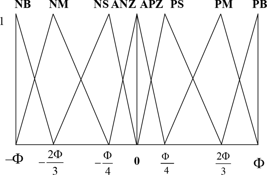
Figure 3. Membership function of ${\boldsymbol{s}}$ .

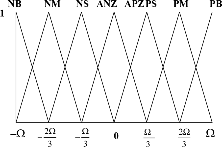
Figure 4. Membership function of ${{\boldsymbol{u}}_3}$ .

3.2. The fast subsystem

The fast subsystem describes the system’s flexible movement. The flexible joints and the flexible link will not only affect the control but also produce vibration. And, their vibration levels are not the same. So, we further decompose the fast subsystem into two independent sub-sub systems: the flexible-joint fast subsystem and the flexible-link fast subsystem. The flexible-joint fast subsystem describes the system’s flexible movement caused by the flexible joints. And, the flexible-link fast subsystem describes the system’s flexible movement caused by the flexible link. The flexible-joint fast subsystem’s controller ${\tau _{\rm f1}}$ is designed to suppress the vibration caused by the flexible joints. The flexible-link fast subsystem’s controller ${\boldsymbol\tau _{\rm f2}}$ is used to suppress the vibration caused by the flexible-link actively. So, the total controller for the fast subsystem is: ${\boldsymbol\tau _{\rm f}} = {\boldsymbol\tau _{\rm f1}} + {\boldsymbol\tau _{\rm f2}}$ .

3.2.1. The flexible-joint fast subsystem

Now, only the influence of the flexible joints is considered. So, let $\boldsymbol\delta = 0$ in Eq. (16), the dynamic equation of the rigid-link and flexible-joints system is obtained as:

(38a) \begin{align}{{\rm{\varepsilon }}^2}{\ddot{{\boldsymbol{z}}}_\rm{\theta }} = - {\boldsymbol{J}}_\rm{\theta } ^{- 1}{{\boldsymbol{K}}_{\rm{\theta } \varepsilon }}{{\boldsymbol{z}}_\rm{\theta } } + {\boldsymbol{J}}_\rm{\theta }^{ - 1}{\boldsymbol\tau _{\rm k1}} - {\ddot{{\boldsymbol{q}}}_\rm{\theta } }\end{align}

(38b) \begin{align}{\ddot{{\boldsymbol{q}}}_\rm{\theta } } = - {\boldsymbol{D}}_{\rm s}^{ - 1}\left( {{{\boldsymbol{C}}_1} - {{\boldsymbol{K}}_{\rm{\theta } \varepsilon }}{{\boldsymbol{z}}_\rm{\theta } }} \right)\end{align}

where ${\boldsymbol\tau _{\rm k1}} = {\boldsymbol\tau _{\rm s}} + {\boldsymbol\tau _{\rm f1}} + {\boldsymbol\tau _{\rm d}}$ .

The feedback controller is designed as following

(39) \begin{align}{\boldsymbol\tau _{\rm f1}} = \frac{{{{\boldsymbol{K}}_{\rm f}}({{\dot{{\boldsymbol{q}}}}_\rm{\theta } } - \dot{\boldsymbol\theta} )}}{{{\varepsilon ^2}}}\end{align}

where ${{\boldsymbol{K}}_{\rm f}} = {{\boldsymbol{K}}_2}/{{\rm{\varepsilon }}^2}$ , ${{\boldsymbol{K}}_2}$ is a positive definite diagonal matrix.

The controller can adjust ${{\boldsymbol{K}}_{\rm f}}$ in time according to the difference of the link’s rotation angular velocity ${\dot{{\boldsymbol{q}}}_\rm{\theta } }$ and the motor rotor’s rotation angular velocity $\dot{\boldsymbol\theta} $ . The stability of the flexible-joint fast subsystem is ensured. Combining with Eq. (38), the flexible-joint fast subsystem’s dynamic equation is:

(40) \begin{align}{{\rm{\varepsilon }}^2}{\ddot{{\boldsymbol{z}}}_\rm{\theta } } = {\boldsymbol{J}}_\rm{\theta } ^{ - 1}({\boldsymbol\tau _{\rm s}} + {\boldsymbol\tau _{\rm d}} - {{\boldsymbol{K}}_{\rm{\theta } \varepsilon }}{{\boldsymbol{z}}_\rm{\theta } } - {{\boldsymbol{J}}_\rm{\theta } }{\ddot{{\boldsymbol{q}}}_\rm{\theta } }) - {\varepsilon ^2}{\boldsymbol{J}}_\rm{\theta } ^{ - 1}{{\boldsymbol{K}}_2}{\dot{{\boldsymbol{z}}}_\rm{\theta } }\end{align}

3.2.2. The flexible-link fast subsystem

Now, only the influence of the flexible link is considered. So let $\boldsymbol\theta = {{\boldsymbol{q}}_\rm{\theta } }$ , $\dot{\boldsymbol\theta} = {\dot{{\boldsymbol{q}}}_\rm{\theta } }$ in Eq. (16), the dynamic equation of the flexible-link and rigid-joints system is obtained as:

(41a) \begin{align}{\ddot{{\boldsymbol{q}}}_\rm{\theta } } = - {\boldsymbol{G}}_{11}^ * {{\boldsymbol{C}}_1} - {\boldsymbol{G}}_{12}^ * {{\boldsymbol{C}}_2} - {\boldsymbol{G}}_{12}^ * {K_{ {\delta } \varepsilon }}{z_{ {\delta }} } + {\boldsymbol{G}}_{11}^ * {\boldsymbol\tau _{\rm k2}}\end{align}

(41b) \begin{align}{{\rm{\varepsilon }}^2}{\ddot{{\boldsymbol{z}}}_{ {\delta }} } = - {\boldsymbol{G}}_{21}^ * {{\boldsymbol{C}}_1} - {\boldsymbol{G}}_{22}^ * {{\boldsymbol{C}}_2} - {\boldsymbol{G}}_{22}^ * {K_{ {\delta } \varepsilon }}{z_{ {\delta }} } + {\boldsymbol{G}}_{21}^ * {\boldsymbol\tau _{\rm k2}}\end{align}

where ${\boldsymbol\tau _{\rm k2}} = {\boldsymbol\tau _{\rm s}} + {\boldsymbol\tau _{\rm f2}} + {\boldsymbol\tau _{\rm d}}$ , $${\boldsymbol{G}}_{11}^* = {\left( {\left[ {\matrix{ {1\quad 0} \cr {0\quad 1} \cr } } \right] + {{\boldsymbol{G}}_{11}}{J_\theta }} \right)^{ - 1}}{{\boldsymbol{G}}_{11}}$$ , $${\boldsymbol{G}}_{12}^* = {\left( {\left[ {\matrix{ {1\quad 0} \cr {0\quad 1} \cr } } \right] + {{\boldsymbol{G}}_{11}}{J_\theta }} \right)^{ - 1}}{{\boldsymbol{G}}_{12}}$$ , $${\boldsymbol{G}}_{21}^* = {{\boldsymbol{G}}_{21}} - {\left( {\left[ {\matrix{ {1\quad 0} \cr {0\quad 1} \cr } } \right] + {{\boldsymbol{G}}_{11}}{J_\theta }} \right)^{ - 1}}{{\boldsymbol{G}}_{21}}{J_\theta }{{\boldsymbol{G}}_{11}}$$ , $${\boldsymbol{G}}_{22}^* = {{\boldsymbol{G}}_{22}} - {\left( {\left[ {\matrix{ {1\quad 0} \cr {0\quad 1} \cr } } \right] + {{\boldsymbol{G}}_{11}}{J_\theta }} \right)^{ - 1}}{{\boldsymbol{G}}_{21}}{J_\theta }{{\boldsymbol{G}}_{12}}$$ .

Definite a fast time variant: ${{\boldsymbol{t}}_{\rm f}} = {\boldsymbol{t}}/{\varepsilon ^2}$ , and its modifications: ${{\boldsymbol{z}}_{\rm f1}} = {{\boldsymbol{z}}_{ {\delta }} } - {\bar{{\boldsymbol{z}}}_{ {\delta }} }$ and ${{\boldsymbol{z}}_{\rm f2}} = {\varepsilon ^2}{\dot{{\boldsymbol{z}}}_{ {\delta }} }$ . In the fast subsystem, the slow variables can be regarded as constants, that is, ${\rm d}{\bar{{\boldsymbol{z}}}_{ {\delta }} }/{\rm d}{{{t}}_{\rm f}} = {\varepsilon ^2}{\dot{\bar{{\boldsymbol{z}}}}_{ {\delta }} } = 0$ . Let ${\rm{\varepsilon }} = 0$ , the dynamic equation of the flexible-link fast subsystem can be obtained as:

(42) \begin{align}\frac{{{\rm d}{{\boldsymbol{Z}}_{\rm f}}}}{{{\rm d}{{{t}}_{\rm f}}}} = {{\boldsymbol{A}}_{\rm f}}{{\boldsymbol{Z}}_{\rm f}} + {{\boldsymbol{B}}_{\rm f}}{\boldsymbol\tau _{\rm f2}}\end{align}

where ${{\boldsymbol{Z}}_{\rm f}} = \left[ {\begin{array}{c}{{{\boldsymbol{z}}_{\rm f1}}}\\[4pt]{{{\boldsymbol{z}}_{\rm f2}}}\end{array}} \right]$ , $${{\boldsymbol{A}}_{\rm{f}}} = \left[ {\matrix{ 0 & {\boldsymbol{I}} \cr { - \overline {\boldsymbol{G}} _{22}^*{{\boldsymbol{K}}_{\delta \varepsilon }}} & 0 \cr } } \right]$$ , ${{\boldsymbol{B}}_{\rm f}} = \left[ {\begin{array}{c}0\\[4pt]{\bar{{\boldsymbol{G}}}_{21}^ * }\end{array}} \right]$ .

Because Eq. (42) is linear controlled, we can adjust the system state variable ${{\boldsymbol{Z}}_{\rm f}}$ using a linear-quadratic optimal controller. It can reach zero to realize the active suppression of the elastic vibration caused by the flexible link. Choosing the performance function of the optimal control: ${{\boldsymbol{J}}_{\rm f}} = \frac{1}{2}\int_0^\infty {({\boldsymbol{Z}}_{\rm f}^{\rm T}} {{\boldsymbol{Q}}_{\rm f}}{{\boldsymbol{Z}}_{\rm f}} + \boldsymbol\tau _{\rm f2}^{\rm T}{{\boldsymbol{R}}_{\rm f}}{\boldsymbol\tau _{\rm f2}}){\rm d}{{\boldsymbol{t}}_{\rm f}}$ , the controller can be designed as:

(43) \begin{align}{\boldsymbol\tau _{\rm f2}} = - {\boldsymbol{R}}_{\rm f}^{ - 1}{\boldsymbol{B}}_{\rm f}^{\rm T}{\boldsymbol{P}}{{\boldsymbol{Z}}_{\rm f}}\end{align}

where ${{\boldsymbol{Q}}_{\rm f}}$ and ${{\boldsymbol{R}}_{\rm f}}$ are symmetric positive definite matrices; ${\boldsymbol{P}}$ is the only solution for the Ricatti equation [Reference Koskie, Couomarbatch and Gajic63]: ${\boldsymbol{P}}{{\boldsymbol{A}}_{f}} + {\boldsymbol{A}}_{f}^T{{\boldsymbol{P}}} - {\boldsymbol{P}}{{\boldsymbol{B}}_{f}}{\boldsymbol{R}}_{f}^{ - 1}{\boldsymbol{B}}_{f}^{T}{\boldsymbol{P}} + {{\boldsymbol{Q}}_{f}} = 0$ .

4. Simulation

We use the proposed hybrid controller to simulate the free-floating flexible-joints and flexible-link space manipulator system shown in Fig. 1. The actual values of the parameters in the system are: ${{{m}}_0} = 40{\rm{kg}}$ , ${{{m}}_1} = 2{\rm{kg}}$ , ${{\rho }} = 1{\rm{kg}}/{\rm m}$ , ${{{l}}_1} = 3{\rm{m}}$ , ${{{l}}_2} = 3{\rm{m}}$ , ${{EI}} = 300{\rm N} \cdot {{\rm m}^2}$ , ${{{J}}_0} = 34.17{\rm{kg}} \cdot {{\rm m}^2}$ , ${{{J}}_1} = 3{\rm{kg}} \cdot {{\rm m}^2}$ , ${{{J}}_{\rm{\theta } 1}} = {{{J}}_{\rm{\theta } 2}} = 0.5{\rm{kg}} \cdot {{\rm m}^2}$ , ${{{k}}_{\rm{\theta } 1}} = {{{k}}_{\rm{\theta } 2}} = 300{\rm N} \cdot {\rm m}/{\rm{rad}}$ . The flexible link is easy to deform, so ${{{l}}_2}$ is uncertain. In the simulation, its estimated value is: ${{{l}}_2} = 2.5{\rm m}$ . The fuzzy parameters are: ${{{\Phi }}_1} = {{{\Phi }}_2} = 1$ , ${{{\Omega }}_1} = {{{\Omega }}_2} = 10$ . The control parameters are: $\lambda = diag(12,12)$ , ${{{l}}_{\rm d}} = 1$ , ${{{l}}_{\rm h}} = 1$ , ${{{l}}_t} = 2$ , ${{\boldsymbol{K}}_2} = {\rm{diag}}(100,100)$ , ${{\boldsymbol{Q}}_{ f}} = {\rm{diag}}(0.1,0.1)$ , ${{\boldsymbol{R}}_{ f}} = {\rm{diag}}(0.01,0.01)$ .

Simulation 1:

First, a simple simulation is taken. The desired trajectories are: ${{{q}}_{0\rm d}} = 0$ , ${{{q}}_{1\rm d}} = 0.1{\rm{rad}}$ , ${{{q}}_{2\rm d}} = 0$ . The initial states are: $${\boldsymbol{q}}(0) = {\left[ {\matrix{ {0.05\quad 0\quad 0.1} \cr } } \right]^{\rm{T}}}{\rm{rad}}$$ , $${\boldsymbol{\theta }}(0) = {\left[ {\matrix{ {0\quad 0.1} \cr } } \right]^{\rm{T}}}{\rm{rad}}$$ , $${\boldsymbol{\delta }}\left( 0 \right) = {\left[ {\matrix{ {0\quad 0} \cr } } \right]^{\rm{T}}}m$$ . The simulation time: ${{t}} = 10{\rm s}$ . None external interference signal.

The simulation results are shown in Figs. 5–8. Figure 5 is the space manipulator trajectory tracking error curve. Figure 6 is the curve of the flexible link’s mode coordinate. Figure 7 is the flexible link’s deformation curve. Figure 8 shows the flexible-joints angle errors. We can see that the system’s trajectory tracking errors converge to zero (the error is only 0.009 rad). The flexible-link’s vibration is suppressed, and its deformation is compensated. The flexible-joints angle errors are decreased. The control is effective.

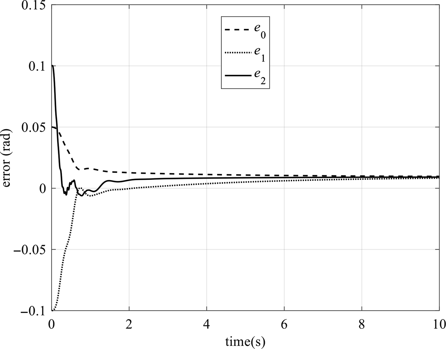
Figure 5. The space manipulator trajectory tracking errors.

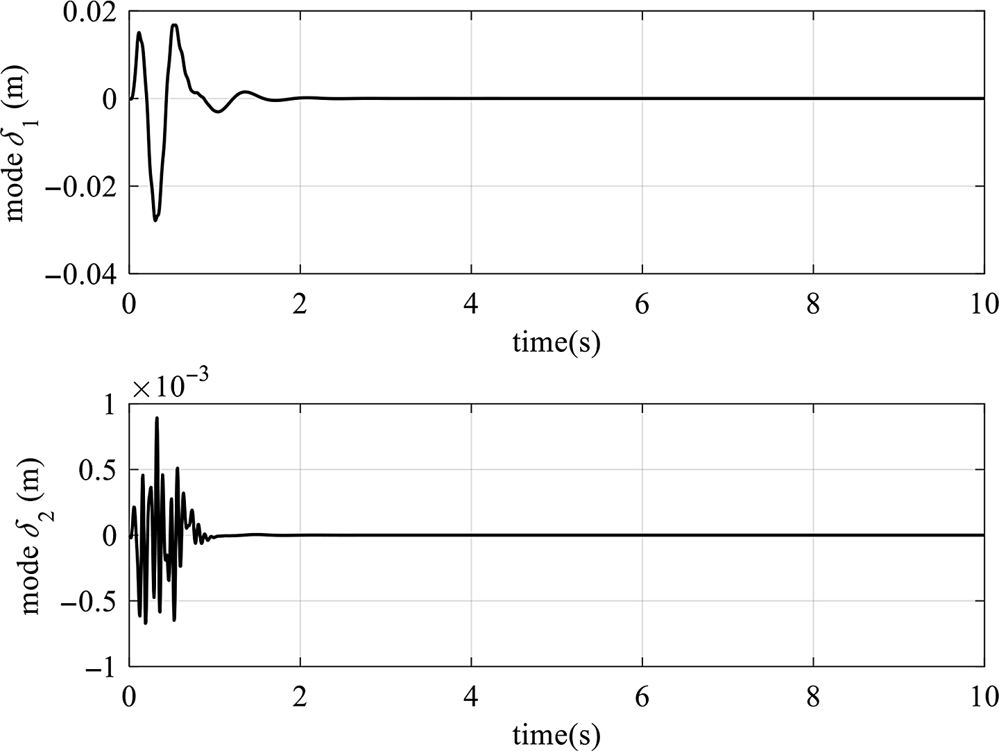
Figure 6. The flexible link’s mode coordinate.

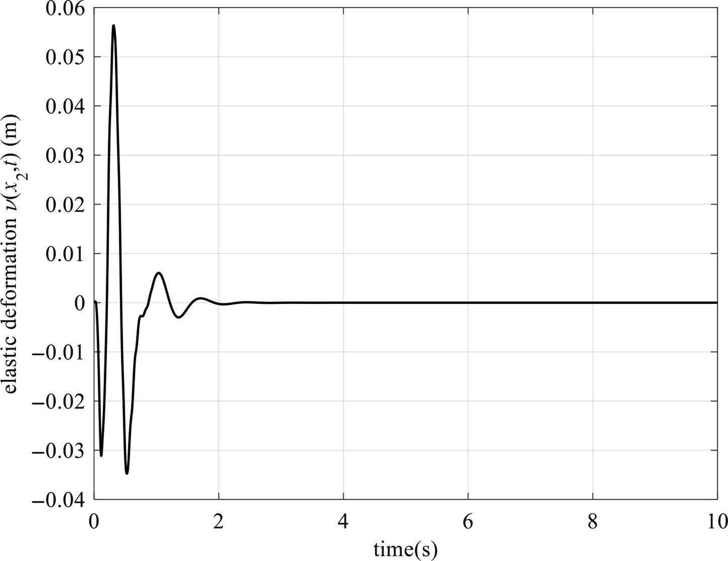
Figure 7. The flexible link’s deformation.

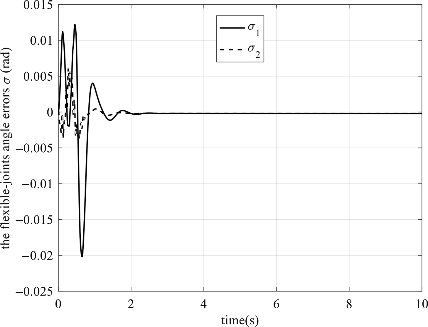
Figure 8. The flexible-joints angle errors $\sigma $ .

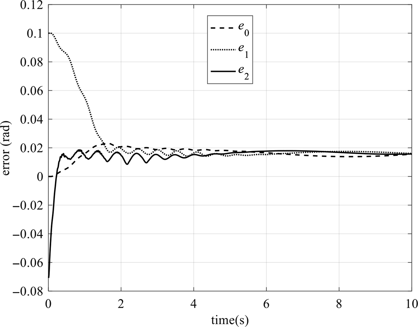
Figure 9. The space manipulator trajectory tracking errors.

But, the desired trajectories are simple, and the external interference is not considered in simulation 1. So, simulation 2 is taken.

Simulation 2:

The desired trajectories are: ${{\rm{q}}_{0{\rm d}}} = \frac{\pi }{4}\left[ {\frac{{\rm{t}}}{{10}} - \frac{1}{{2\pi }}\sin \left( {\frac{\pi }{5}{\rm{t}}} \right)} \right]$ , ${{\rm{q}}_{1{\rm d}}} = \frac{\pi }{2}\left[ {\frac{{\rm{t}}}{{10}} - \frac{1}{{2\pi }}\sin \left( {\frac{\pi }{5}{\rm{t}}} \right)} \right]$ , ${{\rm{q}}_{2{\rm d}}} = \frac{\pi }{2}\left[ {1 - \frac{{\rm{t}}}{{10}} + \frac{1}{{2\pi }}\sin \left( {\frac{\pi }{5}{\rm{t}}} \right)} \right]$ . The initial state is: $${\boldsymbol{q}}(0) = {[\matrix{ {0\quad 0.1\quad 1.5} \cr } ]^{\rm{T}}}{\rm{rad}}$$ , $${\boldsymbol{\theta }}(0) = {[\matrix{ {0.1\quad 1.5} \cr } ]^{\rm{T}}}{\rm{rad}}$$ , $${\boldsymbol{\delta }}\left( 0 \right) = {[\matrix{ {0\quad 0} \cr } ]^{\rm{T}}}m$$ . The simulation time: ${\rm{t}} = 10{\rm s}$ . The external interference signal is: $${{\boldsymbol{\tau }}_{\rm{d}}} = {\left[ {\matrix{ {\sin ({\rm{t}})\quad \cos ({\rm{t}})} \cr } } \right]^{\rm{T}}}{\rm{N}} \cdot {\rm{m}}$$ .

The simulation results are shown in Figs. 9–12. Figure 9 is the space manipulator trajectory tracking error curve. Figure 10 is the curve of the flexible link’s mode coordinate. Figure 11 is the flexible link’s deformation curve. Figure 12 shows the flexible-joints angle errors. The results show that the system can accurately track the desired trajectory (the error is only 0.015 rad). The flexible link’s deformation is compensated. The vibrations caused by the flexible joints and the flexible link can be suppressed.

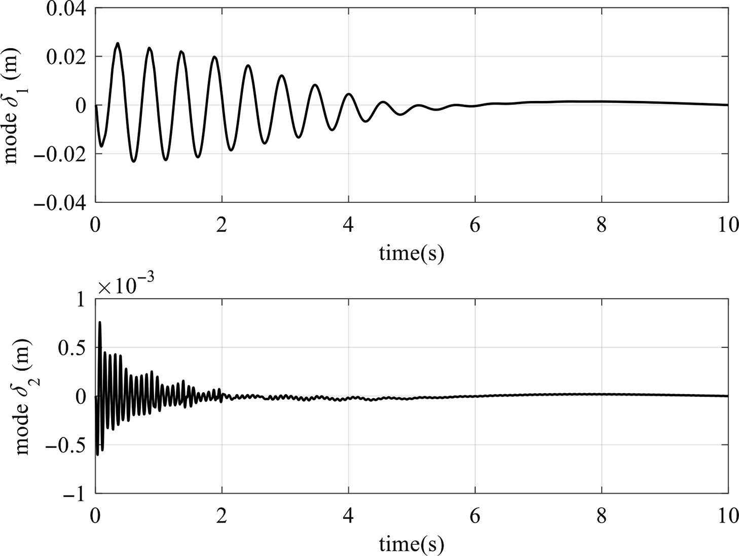
Figure 10. The flexible link’s mode coordinate.

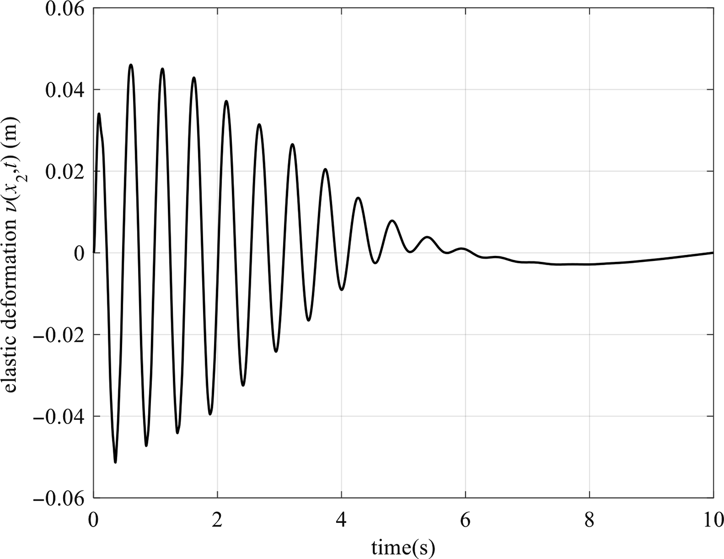
Figure 11. The flexible link’s deformation.

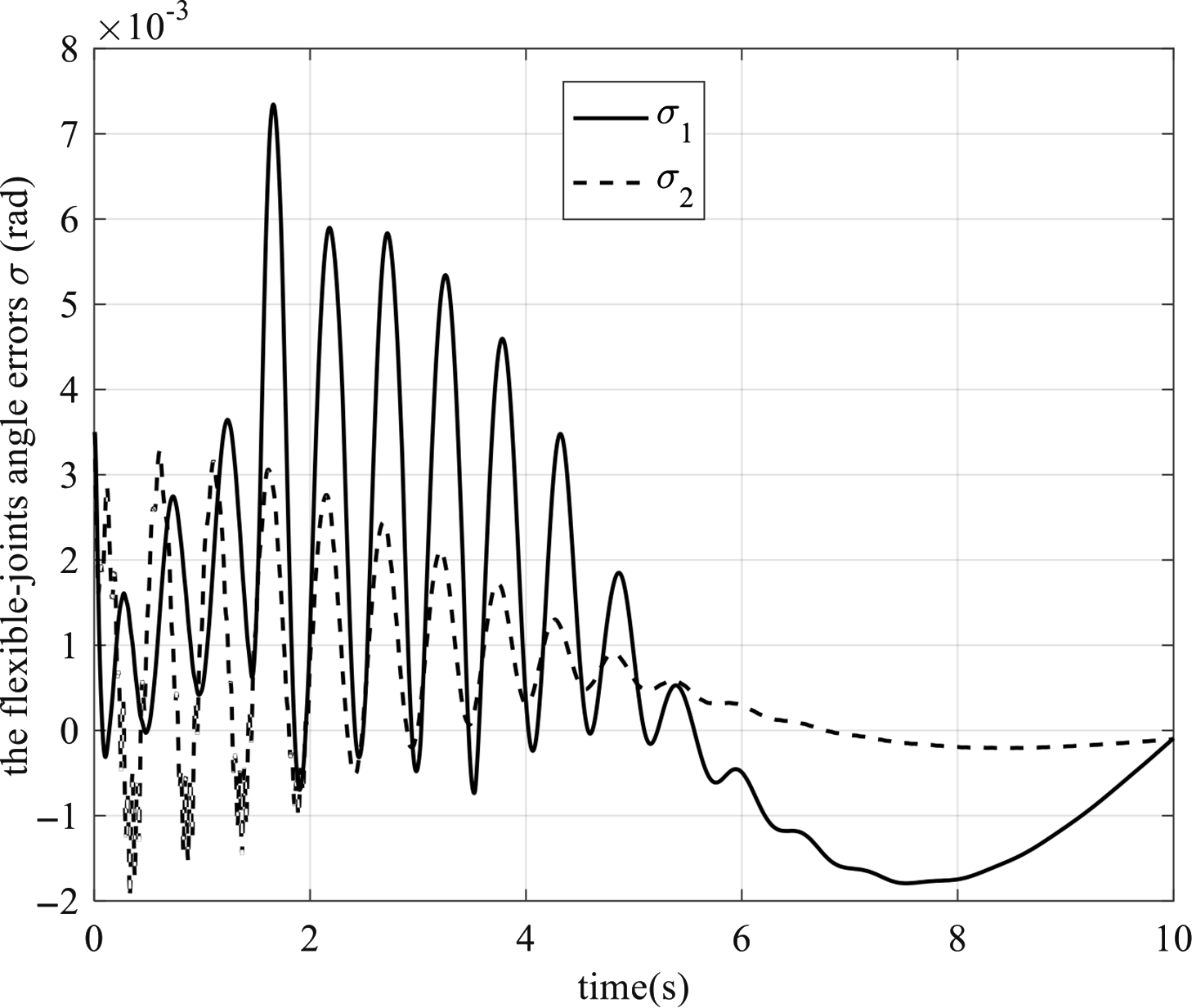
Figure 12. The flexible-joints angle errors $\sigma $ .

The comparison experiments are also taken in simulation 2 to prove the effectiveness of the hybrid control:

Case 1: Turn off the fuzzy controller ${{\boldsymbol{u}}_3}$ . The simulation results are shown in Figs. 13 and 14. We can find that, when ${{\boldsymbol{u}}_3}$ is closed, the system’s tracking errors and the flexible-joints angle errors increase, the control precision decreases.

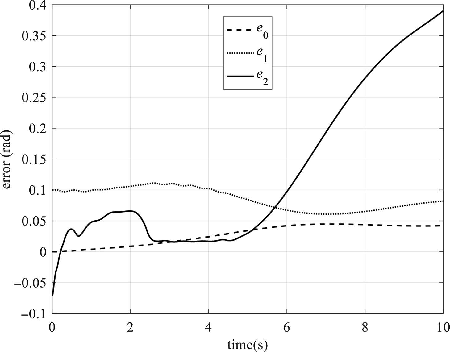
Figure 13. The space manipulator trajectory tracking errors when ${{\boldsymbol{u}}_3}$ is closed.

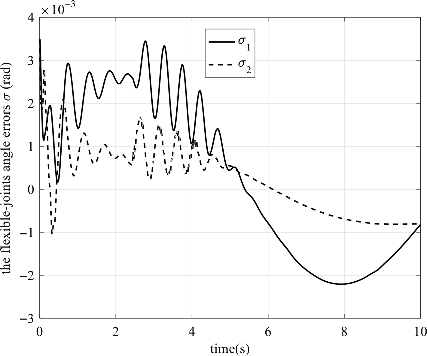
Figure 14. The flexible-joints angle errors $\sigma $ when ${{\boldsymbol{u}}_3}$ is closed.

Case 2: Turn off the fast controller ${\boldsymbol\tau _{\rm f}}$ . The simulation results are shown in Figs. 15–18. We can find that, when ${\boldsymbol\tau _{\rm f}}$ is closed, the trajectory tracking errors and the flexible-joints angle errors became large in <1.2 s, the flexible-link’s vibration cannot be suppressed and its deformation cannot be compensated. That is, the system fails to track. So, the effectiveness of ${\boldsymbol\tau _{\rm f}}$ is proved.

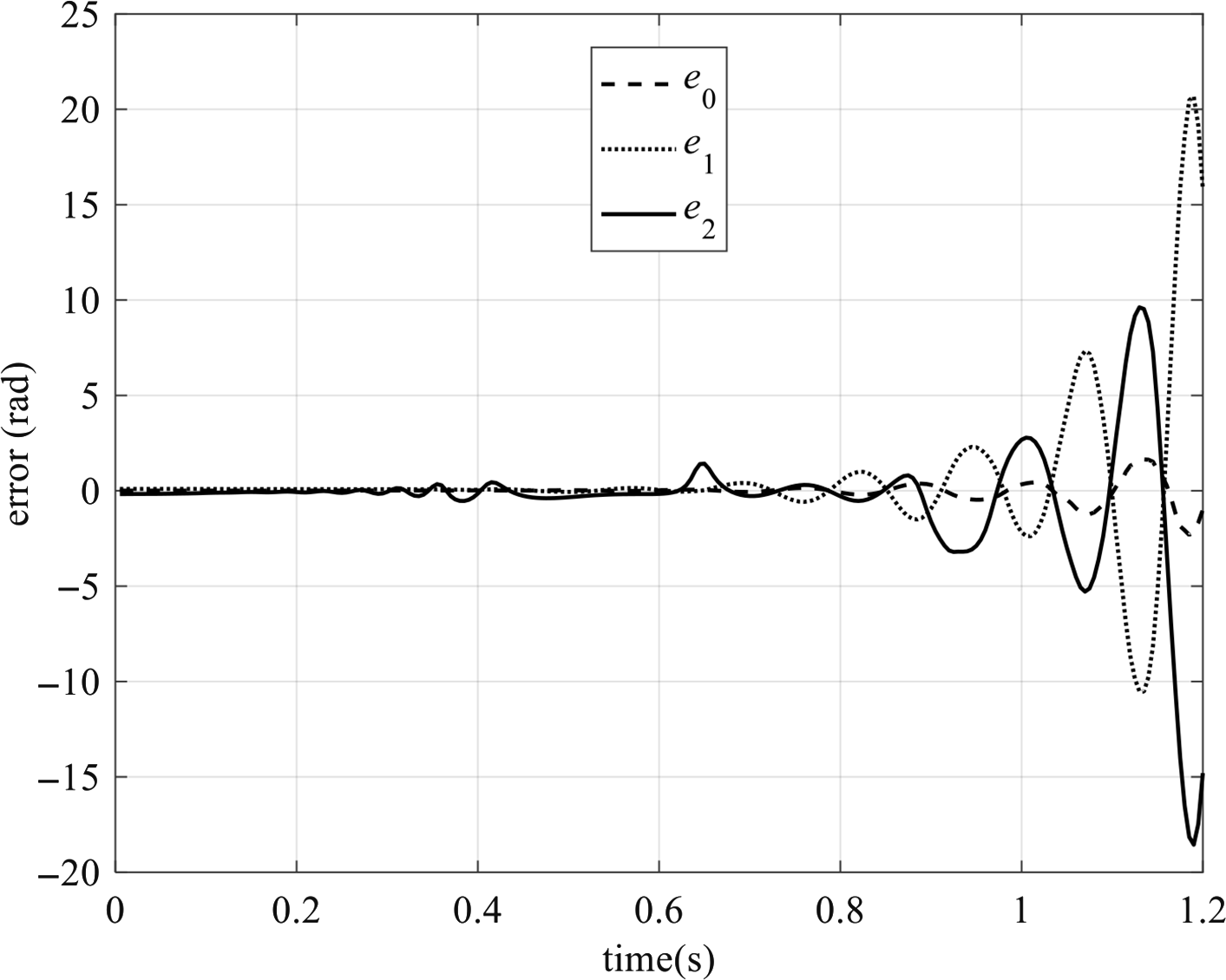
Figure 15. The space manipulator trajectory tracking errors when ${\boldsymbol\tau _{\rm f}}$ is closed.

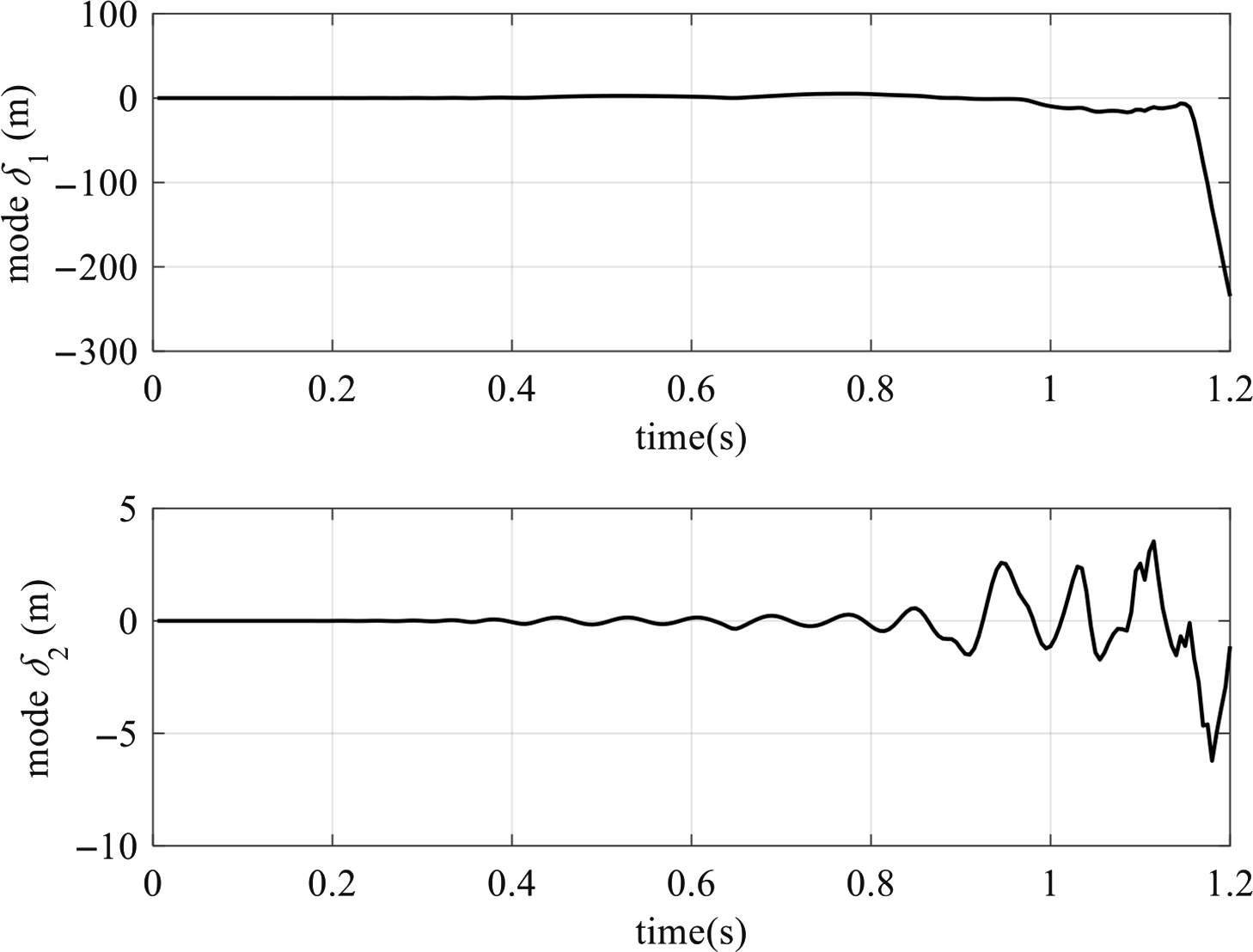
Figure 16. The flexible link’s mode coordinate when ${\boldsymbol\tau _{\rm f}}$ is closed.

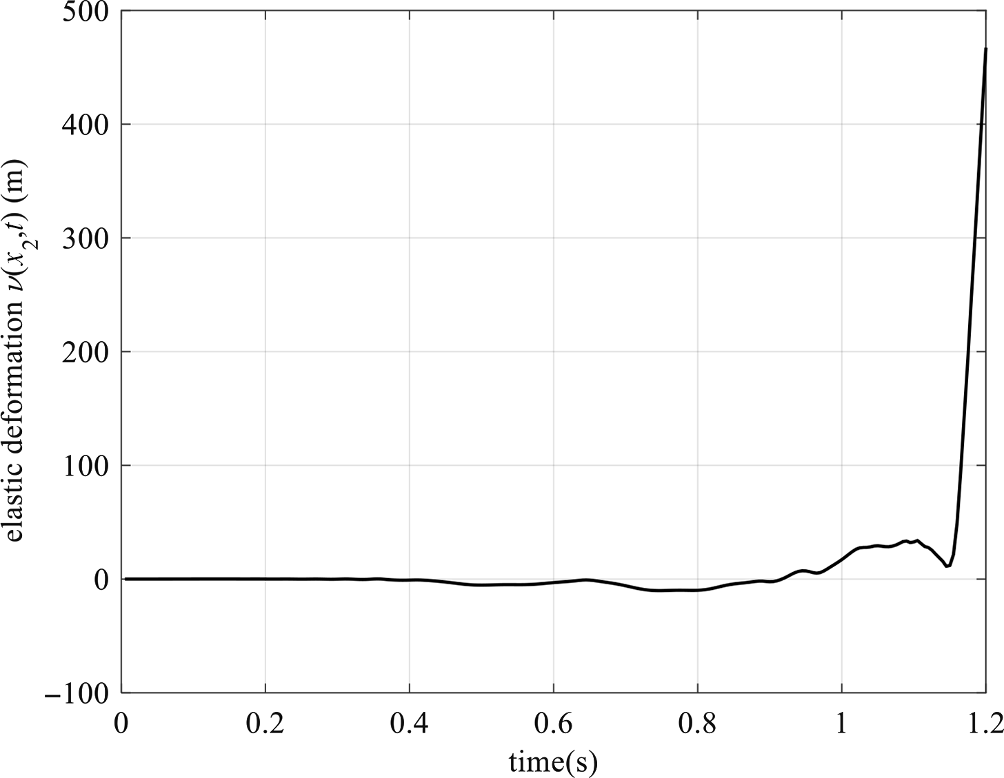
Figure 17. The flexible link’s deformation when ${\boldsymbol\tau _{\rm f}}$ is closed.

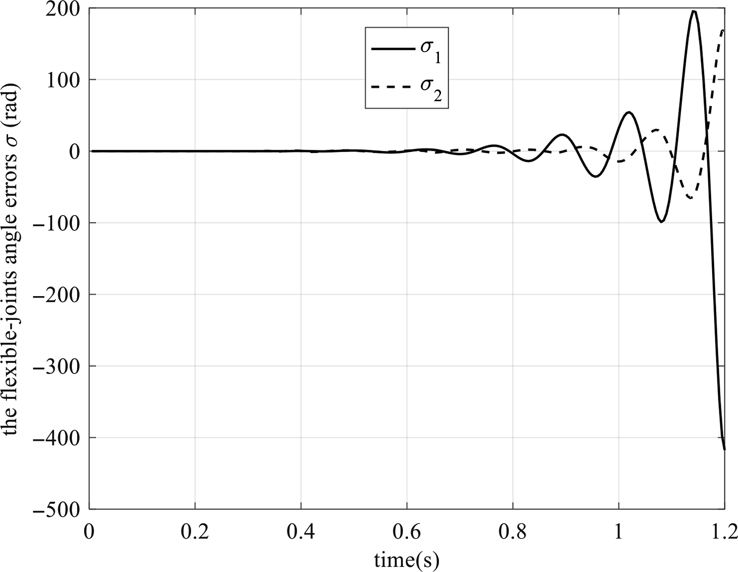
Figure 18. The flexible-joints angle errors $\sigma $ when ${\boldsymbol\tau _{\rm f}}$ is closed.