


1 Introduction
Centrifugal instability, or inertial instability, is the most common instability developing on vortices in a rotating medium. It is a local instability occurring when the balance between the centrifugal force and the pressure gradient is disrupted, i.e. when the square of the absolute angular momentum of the fluid decreases with radius  $r$ in inviscid fluids (Rayleigh Reference Rayleigh1917; Synge Reference Synge1933; Kloosterziel & van Heijst Reference Kloosterziel and van Heijst1991). While this condition applies to axisymmetric disturbances, a generalized criterion for non-axisymmetric perturbations has been derived by Billant & Gallaire (Reference Billant and Gallaire2005).
Linear stability analysis of a columnar vortex with Gaussian angular velocity in inviscid fluids shows that the growth rate is maximum at infinite wavenumber (Smyth & McWilliams Reference Smyth and McWilliams1998). However, as soon as viscous effects are taken into account, short wavelengths are damped and the fastest growing mode has a finite wavenumber (Lazar, Stegner & Heifetz Reference Lazar, Stegner and Heifetz2013; Yim, Billant & Ménesguen Reference Yim, Billant and Ménesguen2016).
Kloosterziel, Carnevale & Orlandi (Reference Kloosterziel, Carnevale and Orlandi2007) and Carnevale et al. (Reference Carnevale, Kloosterziel, Orlandi and Van Sommeren2011) have analysed the nonlinear evolution of the centrifugal instability in a rotating medium at high Reynolds number. They have shown that the vortex saturates to a centrifugally stable state where the Rayleigh instability condition is no longer satisfied, i.e. the square of the axial average of the absolute angular momentum does not decrease with radius. Hence, the instability redistributes the regions of positive and negative absolute angular momentum under the constraint of absolute angular momentum conservation in the inviscid limit.
The saturation of an instability towards a periodic limit cycle for which the mean flow is stable has been recently described by means of a self-consistent approach (Mantič-Lugo et al. Reference Mantič-Lugo, Arratia and Gallaire2014). In this approach, the flow is decomposed into time-averaged mean flow and unsteady perturbations. Then, the nonlinear saturation can be described by computing the mean flow distortion due to the Reynolds stresses of the perturbation and the linear growth of the perturbation on the mean flow. Here, we develop a similar approach for the centrifugal instability using a spatial average instead of a time average since the instability is spatially periodic but not periodic in time.
2 Governing equations
We consider the Carton and McWilliams vortex (Carton, Flierl & Polvani Reference Carton, Flierl and Polvani1989) with angular velocity (figure 1a)
 $$\begin{eqnarray}\unicode[STIX]{x1D6FA}=\unicode[STIX]{x1D6FA}_{0}\exp (-r^{2}/R^{2}),\end{eqnarray}$$
 where  $\unicode[STIX]{x1D6FA}_{0}$ is the maximum angular velocity,
  $r$ the radial coordinate and
  $R$ the radius of the vortex. Such an isolated profile is frequently observed (Ioannou et al. Reference Ioannou, Stegner, Le Vu, Taupier-Letage and Speich2017) and its stability has been extensively studied (Gent & McWilliams Reference Gent and McWilliams1986; Carton et al. Reference Carton, Flierl and Polvani1989; Smyth & McWilliams Reference Smyth and McWilliams1998; Billant & Gallaire Reference Billant and Gallaire2005; Kloosterziel et al. Reference Kloosterziel, Carnevale and Orlandi2007; Yim & Billant Reference Yim and Billant2015). The vortex (2.1) is a steady solution of the Euler equation since it is axisymmetric and axially uniform. It is also an exact solution of the Navier–Stokes equation when
  $\unicode[STIX]{x1D6FA}_{0}$ and
  $R$ are allowed to vary with time as follows:
  $\unicode[STIX]{x1D6FA}_{0}=\unicode[STIX]{x1D6FA}_{i}(R_{i}/R)^{4}$ with
  $R^{2}=R_{i}^{2}+4\unicode[STIX]{x1D708}t$, where
  $\unicode[STIX]{x1D708}$ is the kinematic viscosity,
  $t$ the time and
  $\unicode[STIX]{x1D6FA}_{i}$,
  $R_{i}$ are the initial angular velocity and radius. In the following, the length and time are non-dimensionalized with
  $R$ and
  $1/\unicode[STIX]{x1D6FA}_{0}$, respectively. The governing equations for the velocity field
  $\boldsymbol{u}=[u,v,w]$ in cylindrical coordinates
  $(r,\unicode[STIX]{x1D703},z)$ and pressure
  $p$ read
 $$\begin{eqnarray}\displaystyle & \displaystyle \frac{\unicode[STIX]{x2202}\boldsymbol{u}}{\unicode[STIX]{x2202}t}+\boldsymbol{u}\boldsymbol{\cdot }\unicode[STIX]{x1D735}\boldsymbol{u}+2Ro^{-1}\boldsymbol{e}_{z}\times \boldsymbol{u}=-\unicode[STIX]{x1D735}p+Re^{-1}\unicode[STIX]{x1D6FB}^{2}\boldsymbol{u}, & \displaystyle\end{eqnarray}$$
 $$\begin{eqnarray}\displaystyle & \displaystyle \unicode[STIX]{x1D735}\boldsymbol{\cdot }\boldsymbol{u}=0, & \displaystyle\end{eqnarray}$$
 where  $e_{z}$ is the unit vector in
  $z$ direction and the Reynolds and Rossby numbers are defined as
  $Re=\unicode[STIX]{x1D6FA}_{0}R^{2}/\unicode[STIX]{x1D708}$ and
  $Ro=2\unicode[STIX]{x1D6FA}_{0}/f$, respectively, with
  $f$ the Coriolis parameter measuring the background rotation about the
  $z$ axis. The divergence-free condition (2.3) is not further written in the following sections but is always guaranteed.
2.1 Linear stability
The linear stability of the base flow (2.1) has been first studied by linearizing (2.2)–(2.3) and assuming infinitesimal perturbations with axial wavenumber  $k$, azimuthal wavenumber
  $m$ and growth rate
  $\unicode[STIX]{x1D70E}$:
 $$\begin{eqnarray}[\tilde{\boldsymbol{u}},\tilde{p}](r,\unicode[STIX]{x1D703},z,t)=[\boldsymbol{u},p](r)\text{e}^{\unicode[STIX]{x1D70E}t+\text{i}kz+\text{i}m\unicode[STIX]{x1D703}}+\text{c.c.},\end{eqnarray}$$
where c.c. indicates the complex conjugate, and gives
 $$\begin{eqnarray}\unicode[STIX]{x1D70E}\boldsymbol{u}+{\mathcal{L}}_{m,k}(\boldsymbol{u}_{b})\boldsymbol{u}=0,\end{eqnarray}$$
where
 $$\begin{eqnarray}{\mathcal{L}}_{m,k}(\boldsymbol{u}_{b})\boldsymbol{u}\equiv \boldsymbol{u}_{b}\boldsymbol{\cdot }\unicode[STIX]{x1D735}_{m,k}\boldsymbol{u}+\boldsymbol{u}\boldsymbol{\cdot }\unicode[STIX]{x1D735}\boldsymbol{u}_{b}+2Ro^{-1}\boldsymbol{e}_{z}\times \boldsymbol{u}+\unicode[STIX]{x1D735}_{m,k}p-Re^{-1}\unicode[STIX]{x1D6FB}_{m,k}^{2}\boldsymbol{u},\end{eqnarray}$$
 where  $\boldsymbol{u}_{b}=[0,r\unicode[STIX]{x1D6FA},0]$. Here,
  $\unicode[STIX]{x1D735}_{m,k}$ and
  $\unicode[STIX]{x1D6FB}_{m,k}^{2}$ are, respectively, the gradient and Laplacian in cylindrical coordinates with the azimuthal derivative replaced by
  $\text{i}m$ and the vertical derivative by
  $\text{i}k$.

Figure 1. (a) Angular velocity ( $\unicode[STIX]{x1D6FA}$) and axial vorticity (
 $\unicode[STIX]{x1D701}$) of the base flow. (b) Linear growth rate as a function of the vertical wavenumber
  $k$ for different azimuthal wavenumbers:
  $m=0$ (solid lines),
  $m=1$ (dashed lines),
  $m=2$ (dotted lines) for
  $Re=800$ (black lines) and
  $Re=2000$ (grey lines) for
  $Ro=-4$. The circles indicate the most unstable modes. (c) Most unstable eigenmode for
  $Re=800$. The shaded area indicates the region where
  $\unicode[STIX]{x1D719}<0$.
In the inviscid limit, the necessary and sufficient condition for the instability of axisymmetric perturbations is that the Rayleigh discriminant  $\unicode[STIX]{x1D719}$ is negative (Rayleigh Reference Rayleigh1917; Synge Reference Synge1933; Kloosterziel & van Heijst Reference Kloosterziel and van Heijst1991):
 $$\begin{eqnarray}\unicode[STIX]{x1D719}\equiv 2\left(\frac{v}{r}+\frac{1}{Ro}\right)\left(\unicode[STIX]{x1D701}+\frac{2}{Ro}\right)<0.\end{eqnarray}$$
 For the base flow (2.1), (2.7) is satisfied when  $Ro<-1$ or
  $Ro>\exp (2)$. Figure 1(b) shows the linear growth rate
  $\unicode[STIX]{x1D70E}$ as a function of
  $k$ for different azimuthal wavenumbers
  $m$ for
  $Ro=-4$ for two different Reynolds numbers,
  $Re=800$ and
  $Re=2000$. The growth rate is maximum for the axisymmetric mode at
  $k_{m}=5.6$ for
  $Re=800$ and
  $k_{m}=8.6$ for
  $Re=2000$. As predicted by the generalized criterion of Billant & Gallaire (Reference Billant and Gallaire2005), only the first non-axisymmetric modes
  $m=1$ and
  $m=2$ are unstable, and their maximum growth rate is lower than for
  $m=0$. Hence, in the following, we will focus on the axisymmetric mode at the most amplified vertical wavenumber
  $k_{m}$. Figure 1(c) shows the most unstable eigenmode for
  $Re=800$,
  $Ro=-4$. It is mostly localized in the region where the Rayleigh discriminant is negative (shaded area).
3 Semilinear formulation
We decompose the flow as
 $$\begin{eqnarray}\boldsymbol{u}(r,\unicode[STIX]{x1D703},z,t)=\overline{\boldsymbol{u}}(r,\unicode[STIX]{x1D703},t)+\hat{\boldsymbol{u}}(r,\unicode[STIX]{x1D703},z,t),\end{eqnarray}$$
 where  $\overline{\boldsymbol{u}}=z_{max}^{-1}\int _{0}^{z_{max}}\boldsymbol{u}\,\text{d}z$ is the axially averaged mean flow over the axial length
  $z_{max}$ (see § 3.3) and
  $\hat{\boldsymbol{u}}$ the perturbation which is not assumed to be small as in the linear stability analysis. Averaging (2.2) in
  $z$ leads to
 $$\begin{eqnarray}\frac{\unicode[STIX]{x2202}\overline{\boldsymbol{u}}}{\unicode[STIX]{x2202}t}+\overline{\boldsymbol{u}}\boldsymbol{\cdot }\unicode[STIX]{x1D735}\overline{\boldsymbol{u}}+2Ro^{-1}\boldsymbol{e}_{z}\times \overline{\boldsymbol{u}}+\unicode[STIX]{x1D735}\overline{p}-Re^{-1}\unicode[STIX]{x1D6FB}^{2}\overline{\boldsymbol{u}}=-\overline{\hat{\boldsymbol{u}}\boldsymbol{\cdot }\unicode[STIX]{x1D735}\hat{\boldsymbol{u}}}.\end{eqnarray}$$
 Subtracting (3.2) from (2.2) yields the equation for the perturbation  $\hat{\boldsymbol{u}}$:
 $$\begin{eqnarray}\frac{\unicode[STIX]{x2202}\hat{\boldsymbol{u}}}{\unicode[STIX]{x2202}t}+\overline{\boldsymbol{u}}\boldsymbol{\cdot }\unicode[STIX]{x1D735}\hat{\boldsymbol{u}}+\hat{\boldsymbol{u}}\boldsymbol{\cdot }\unicode[STIX]{x1D735}\overline{\boldsymbol{u}}+2Ro^{-1}\boldsymbol{e}_{z}\times \hat{\boldsymbol{u}}+\unicode[STIX]{x1D735}\hat{p}-Re^{-1}\unicode[STIX]{x1D6FB}^{2}\hat{\boldsymbol{u}}=-\hat{\boldsymbol{u}}\boldsymbol{\cdot }\unicode[STIX]{x1D735}\hat{\boldsymbol{u}}+\overline{\hat{\boldsymbol{u}}\boldsymbol{\cdot }\unicode[STIX]{x1D735}\hat{\boldsymbol{u}}}.\end{eqnarray}$$
 These mean and fluctuation equations are similar to those of the Reynolds decomposition (Reynolds & Hussain Reference Reynolds and Hussain1972). They involve several coupling terms between the mean and the fluctuation. The right-hand side of (3.2) is the Reynolds stress due to the fluctuations, which acts as forcing or added momentum to the nonlinear mean flow equation (left-hand side of (3.2)). The amplitude of this forcing is proportional to the square of the fluctuation amplitude. In turn, the fluctuation in (3.3) is affected by the evolution of the mean flow through the advection operator ( $\overline{\boldsymbol{u}}\boldsymbol{\cdot }\unicode[STIX]{x1D735}\hat{\boldsymbol{u}}+\hat{\boldsymbol{u}}\boldsymbol{\cdot }\unicode[STIX]{x1D735}\overline{\boldsymbol{u}}$). The fluctuation also evolves due to nonlinear effects with zero mean (right-hand side of (3.3)) (Mantič-Lugo et al. Reference Mantič-Lugo, Arratia and Gallaire2014, Reference Mantič-Lugo, Arratia and Gallaire2015).
3.1 Single harmonic
We introduce now the normal mode form of the perturbation for  $m=0$:
  $\hat{\boldsymbol{u}}(r,\unicode[STIX]{x1D703},z,t)\equiv \hat{\boldsymbol{u}}(r,z,t)\simeq \boldsymbol{u}_{1}(r,t)\text{exp}(\text{i}k_{m}z)+\text{c.c.}$ where
  $k_{m}$ is the most amplified wavenumber obtained from the linear stability analysis. At
  $t=0$, the perturbation is set as
  $\boldsymbol{u}_{1}(r,0)=A_{0}\boldsymbol{u}_{m}$ where
  $\boldsymbol{u}_{m}$ is the dominant eigenmode and
  $A_{0}$ the initial amplitude of the perturbation. Neglecting the higher harmonics, the governing equations (3.2)–(3.3) reduce to
 $$\begin{eqnarray}\displaystyle & \displaystyle \frac{\unicode[STIX]{x2202}\overline{\boldsymbol{u}}}{\unicode[STIX]{x2202}t}+\overline{\boldsymbol{u}}\boldsymbol{\cdot }\unicode[STIX]{x1D735}\overline{\boldsymbol{u}}+2Ro^{-1}\boldsymbol{e}_{z}\times \overline{\boldsymbol{u}}+\unicode[STIX]{x1D735}\overline{p}-Re^{-1}\unicode[STIX]{x1D6FB}^{2}\overline{\boldsymbol{u}}=-\unicode[STIX]{x1D709}(\boldsymbol{u}_{1}), & \displaystyle\end{eqnarray}$$
 $$\begin{eqnarray}\displaystyle & \displaystyle \frac{\unicode[STIX]{x2202}\boldsymbol{u}_{1}}{\unicode[STIX]{x2202}t}+{\mathcal{L}}_{0,k}(\overline{\boldsymbol{u}})\boldsymbol{u}_{1}=0, & \displaystyle\end{eqnarray}$$
 where  ${\mathcal{L}}_{0,k}(\overline{\boldsymbol{u}})$ is a linear operator defined in (2.6) with
  $m=0$ and
  $\unicode[STIX]{x1D709}(\boldsymbol{u}_{1})=\boldsymbol{u}_{1}\boldsymbol{\cdot }\unicode[STIX]{x1D735}_{-k}\boldsymbol{u}_{1}^{\ast }+\boldsymbol{u}_{1}^{\ast }\boldsymbol{\cdot }\unicode[STIX]{x1D735}_{k}\boldsymbol{u}_{1}$ is the Reynolds stress. It is worth mentioning that (3.4)–(3.5) are now only a function of time and the radial coordinate
  $r$. In addition, the divergence-free condition reduces to
  $(1/r)\unicode[STIX]{x2202}r\overline{u}/\unicode[STIX]{x2202}r=0$ since
  $\unicode[STIX]{x2202}\overline{w}/\unicode[STIX]{x2202}z=0$ due to the axial averaging. This implies
  $\overline{u}=0$. It can also be shown that
  $\overline{w}$ remains identically zero for all time if
  $\overline{w}=0$ at
  $t=0$, since the Reynolds stress in the
  $z$-direction is zero. Thus, the mean flow has only a component along the azimuthal direction
  $\overline{\boldsymbol{u}}=[0,\overline{v},0]^{\text{T}}$. Hence, (3.4) simplifies to
 $$\begin{eqnarray}\frac{\unicode[STIX]{x2202}\overline{v}}{\unicode[STIX]{x2202}t}=Re^{-1}\left[\frac{\unicode[STIX]{x2202}^{2}\overline{v}}{\unicode[STIX]{x2202}r^{2}}+\frac{1}{r}\frac{\unicode[STIX]{x2202}\overline{v}}{\unicode[STIX]{x2202}r}-\frac{\overline{v}}{r^{2}}\right]-\unicode[STIX]{x1D709}(\boldsymbol{u}_{1})_{\unicode[STIX]{x1D703}},\end{eqnarray}$$
 which is a simple diffusion equation with a source term independent from the Rossby number  $Ro$. Using the axisymmetry of the mean flow and of the perturbation, (3.5) can also be further reduced to
 $$\begin{eqnarray}\displaystyle & \displaystyle \frac{\unicode[STIX]{x2202}\unicode[STIX]{x1D702}_{1}}{\unicode[STIX]{x2202}t}-\left(\frac{2\overline{v}}{r}+2Ro^{-1}\right)\text{i}kv_{1}-Re^{-1}\left[\frac{\unicode[STIX]{x2202}^{2}\unicode[STIX]{x1D702}_{1}}{\unicode[STIX]{x2202}r^{2}}+\frac{1}{r}\frac{\unicode[STIX]{x2202}\unicode[STIX]{x1D702}_{1}}{\unicode[STIX]{x2202}r}-\frac{\unicode[STIX]{x1D702}_{1}}{r^{2}}-k^{2}\unicode[STIX]{x1D702}_{1}\right]=0, & \displaystyle\end{eqnarray}$$
 $$\begin{eqnarray}\displaystyle & \displaystyle \frac{\unicode[STIX]{x2202}v_{1}}{\unicode[STIX]{x2202}t}+(\overline{\unicode[STIX]{x1D701}}+2Ro^{-1})u_{1}-Re^{-1}\left[\frac{\unicode[STIX]{x2202}^{2}v_{1}}{\unicode[STIX]{x2202}r^{2}}+\frac{1}{r}\frac{\unicode[STIX]{x2202}v_{1}}{\unicode[STIX]{x2202}r}-\frac{v_{1}}{r^{2}}-k^{2}v_{1}\right]=0, & \displaystyle\end{eqnarray}$$
 $\unicode[STIX]{x1D702}_{1}=\unicode[STIX]{x2202}_{z}u_{1}-\unicode[STIX]{x2202}_{r}w_{1}=\text{i}ku_{1}-(\text{i}/kr)\unicode[STIX]{x2202}_{r}((1/r)\unicode[STIX]{x2202}_{r}ru_{1})$ is the azimuthal component of vorticity.
Therefore, our model consists of the semilinear one-dimensional equation (3.5), or equivalently (3.7), for the evolution of the perturbation over the mean flow coupled to (3.6) for the evolution of the mean flow under the effects of the Reynolds stresses of the perturbation and viscous diffusion. The only difference compared to pure linear equations is this evolution of the mean flow. Such a semilinear model is similar to the self-consistent model proposed by Mantič-Lugo et al. (Reference Mantič-Lugo, Arratia and Gallaire2014). The main difference is that the Reynolds decomposition (Reynolds & Hussain Reference Reynolds and Hussain1972) to separate the flow into a mean flow and a fluctuation is here based on spatial axial average, since the perturbation is harmonic along the axis, while the self-consistent model relies upon a time average because the perturbation is harmonic in time for the flows they have considered. Another difference is that the perturbation equations are here simply integrated in time, while, in the self-consistent model, an eigenvalue problem has to be solved after each variation of the mean flow.
3.2 Two harmonics
One can easily include higher harmonics of the fundamental mode following the same approach. For instance, taking into account the second harmonic in the velocity perturbation:  $\hat{\boldsymbol{u}}=\boldsymbol{u}_{1}(r,t)\text{exp}(\text{i}k_{m}z)+\boldsymbol{u}_{2}(r,t)\text{exp}(\text{i}2k_{m}z)+\text{c.c.}$, the perturbation equations become
 $$\begin{eqnarray}\displaystyle & \displaystyle \frac{\unicode[STIX]{x2202}\boldsymbol{u}_{1}}{\unicode[STIX]{x2202}t}+{\mathcal{L}}_{0,k}(\overline{\boldsymbol{u}})\boldsymbol{u}_{1}=-(\boldsymbol{u}_{2}\boldsymbol{\cdot }\unicode[STIX]{x1D735}_{-k}\boldsymbol{u}_{1}^{\ast }+\boldsymbol{u}_{1}^{\ast }\boldsymbol{\cdot }\unicode[STIX]{x1D735}_{2k}\boldsymbol{u}_{2}), & \displaystyle\end{eqnarray}$$
 $$\begin{eqnarray}\displaystyle & \displaystyle \frac{\unicode[STIX]{x2202}\boldsymbol{u}_{2}}{\unicode[STIX]{x2202}t}+{\mathcal{L}}_{0,2k}(\overline{\boldsymbol{u}})\boldsymbol{u}_{2}=-(\boldsymbol{u}_{1}\boldsymbol{\cdot }\unicode[STIX]{x1D735}_{k}\boldsymbol{u}_{\mathbf{1}}). & \displaystyle\end{eqnarray}$$
 $$\begin{eqnarray}\frac{\unicode[STIX]{x2202}\overline{v}}{\unicode[STIX]{x2202}t}=Re^{-1}\left[\frac{\unicode[STIX]{x2202}^{2}\overline{v}}{\unicode[STIX]{x2202}r^{2}}+\frac{1}{r}\frac{\unicode[STIX]{x2202}\overline{v}}{\unicode[STIX]{x2202}r}-\frac{\overline{v}}{r^{2}}\right]-\unicode[STIX]{x1D709}(\boldsymbol{u}_{1})_{\unicode[STIX]{x1D703}}-\unicode[STIX]{x1D709}(\boldsymbol{u}_{2})_{\unicode[STIX]{x1D703}}.\end{eqnarray}$$
 Higher harmonics  $3k_{m},4k_{m},\ldots$ can be taken into account similarly. Since the perturbations equations are integrated in time, there is no particular complexity arising when several harmonics are considered. This is in contrast to the self-consistent model (Mantič-Lugo et al. Reference Mantič-Lugo, Arratia and Gallaire2014) where the eigenvalue problems become increasingly complicated when more than one harmonic is considered (Meliga Reference Meliga2017).
3.3 Numerical method
The semilinear numerical simulations have been performed with the FreeFEM++ software (Hecht Reference Hecht2012) for axisymmetric cylindrical coordinates ( $r,z$). The velocity and pressure are discretized with Taylor–Hood P2 and P1 elements, respectively. The time is discretized using the first-order backward Euler formula. The total number of degrees of freedom is
  $4687$. Three-dimensional (3-D) direct numerical simulations (DNS) have been performed using the open source spectral element code Nek5000 (Fischer, Lottes & Kerkemeier Reference Fischer, Lottes and Kerkemeier2008) in Cartesian coordinates (
 $x,y,z$) in cylindrical geometry. The domain is discretized by 120 000 hexahedral elements and each element is composed of
  $8$ (velocity) or
  $6$ (pressure) Gauss–Lobatto–Legendre quadrature points along each direction (resulting in 250 million degrees of freedom, i.e. 50 000 times more than for the semilinear models). The time and the nonlinear convection terms are discretized using third-order backward differentiation and third-order explicit extrapolation formula, respectively.
Both DNS and semilinear models are initialized with the perturbation $\hat{\boldsymbol{u}}=A_{0}\boldsymbol{u}_{m}\text{exp}(\text{i}k_{m}z)+\text{c.c.}$ where
  $A_{0}=0.001$ is the initial amplitude and
  $\boldsymbol{u}_{m}$ is the most unstable linear eigenmode (figure 1c) obtained by means of the restarted Arnoldi method. The eigenmodes have been normalized so that the absolute maximum value of the vertical velocity is unity,
  $\max (|w_{m}|)=1$ such that
  $\max (|{\hat{w}}|)=A_{0}$.
The domain size for the semilinear model is chosen to be  $r=[0,r_{max}]$ where
  $r_{max}=8$. Since the base angular velocity decays exponentially with
  $r^{2}$, the radial extent does not need to be large: the eigenvalues and eigenvectors are converged as soon as
  $r_{max}>5$. Periodic boundary conditions are applied on
  $z=0$ and
  $z=z_{max}$. The boundary conditions at
  $r=0$ are
  $u=v=0$ since the flow is axisymmetric (Batchelor & Gill Reference Batchelor and Gill1962). At
  $r=r_{max}$, all perturbations are enforced to vanish. The domain sizes in the DNS are
  $r=[-8,8]$ along the horizontal with no-slip boundary conditions and
  $z=[0,13\times 2\unicode[STIX]{x03C0}/k_{m}]$ along the vertical with periodic boundary conditions. To validate the numerical methods, some DNS and simulations with the semilinear models have also been performed with an independent pseudo-spectral code NS3D (Deloncle, Billant & Chomaz Reference Deloncle, Billant and Chomaz2008). Identical results have been obtained.
4 Results
We consider a single Rossby number  $Ro=-4$. This value has been chosen to be sufficiently far from the marginal stability limit
  $Ro=-1$ so that the initial growth rate and nonlinear effects are not weak. In other words, we are not in a weakly nonlinear regime as assumed to derive asymptotically amplitude equations. Two Reynolds numbers will be investigated:
  $Re=800$ and
  $Re=2000$, corresponding to different viscous damping and, thus, to different values of the initial growth rates (figure 1b). This allows us to test the semilinear models for two representative cases where nonlinear effects and higher harmonics are expected to be moderate (
 $Re=800$) or more significant (
 $Re=2000$). Alternatively, different growth rates could have been obtained by varying
  $Ro$ with
  $Re$ fixed.
4.1 Three-dimensional DNS
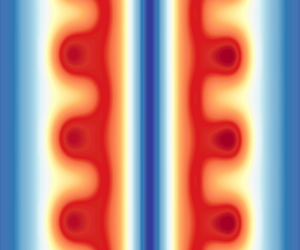
Figure 2 shows snapshots of the azimuthal velocity  $v$ in a DNS for
  $Ro=-4$ and
  $Re=800$. Only two wavelengths are displayed, although the computation is performed over 13 wavelengths. The vertical lines delimit the regions where the Rayleigh discriminant
  $\bar{\unicode[STIX]{x1D719}}$ is negative, where
  $\bar{\unicode[STIX]{x1D719}}$ is based on the axially averaged azimuthal velocity
  $\bar{v}(t,r)$. At
  $t=10$, a slight deformation can be seen in the region where
  $\bar{\unicode[STIX]{x1D719}}<0$. Subsequently, the perturbation grows and rearranges the distribution of azimuthal velocity (
 $20<t<30$). For
  $t>30$, the ‘mushrooms’ start to fade out. Finally, vertical deformations are no longer visible by
  $t=100$ so that the vortex then evolves only by viscous diffusion.

Figure 2. Vertical cross-sections at  $x=0$ of the evolution of the azimuthal velocity field
  $v$ in DNS for
  $k_{m}=5.6$,
  $Ro=-4$,
  $Re=800$. The dashed lines delimit the regions where
  $\bar{\unicode[STIX]{x1D719}}<0$, based on the mean azimuthal velocity
  $\bar{v}$. Only two wavelengths are shown whereas the full domain contains 13 wavelengths along the vertical (see § 3.3).
The solid lines in figure 3(a) show the evolution of the corresponding mean azimuthal velocity  $\bar{v}$. The mean flow profile first decays by viscous diffusion until
  $t=10$. A distortion of the mean flow due to the instability can be seen at
  $t=20$. At
  $t=30$ and
  $t=40$, it becomes strong and the profile exhibits two distinct peaks near
  $r=0.4$ and
  $r=1$. Then, the peak at
  $r\sim 0.4$ disappears and the mean azimuthal velocity profile becomes linear for
  $r<1$ for
  $t>60$. During this process, the maximum velocity has decreased from
  $\max (\bar{v}(t=0))=0.47$ to
  $\max (\bar{v}(t=80))=0.23$ and the corresponding radius has moved from
  $r=0.7$ to
  $r=1.2$. The corresponding Rayleigh discriminant is shown in figure 3(b) (solid lines). At
  $t=0$,
  $\bar{\unicode[STIX]{x1D719}}$ is minimum at
  $r=0.95$ and is negative for
  $0.75<r<1.18$. For
  $t=20$, the region where
  $\bar{\unicode[STIX]{x1D719}}<0$ has enlarged, but the minimum of
  $\bar{\unicode[STIX]{x1D719}}$ has decreased in absolute value. At
  $t=30$, there exist two regions where
  $\bar{\unicode[STIX]{x1D719}}<0$: near
  $r=0.3$ and
  $r=0.8$, while between these regions
  $\bar{\unicode[STIX]{x1D719}}>0$. The minimum value decreases and then increases again subsequently. By comparing figures 3(a) and 3(b), we can see that the mean flow is mostly deformed near the negative peaks of
  $\bar{\unicode[STIX]{x1D719}}$, at least until
  $t=40$. At
  $t=60$,
  $\min (\bar{\unicode[STIX]{x1D719}})$ is no longer negative.

Figure 3. (a) Mean azimuthal velocity  $\bar{v}$ from DNS (solid lines) and the semilinear model with single harmonic (SL-1
 $k_{m}$) (dashed lines). (b) Corresponding Rayleigh discriminant
  $\bar{\unicode[STIX]{x1D719}}$ and (c) perturbation amplitudes
  $A$ as a function of time for
  $Ro=-4$ and
  $Re=800$.

Figure 4. Evolution of the azimuthal velocity (a–c) and axial velocity (d–f) in a DNS for  $k_{m}=8.6$,
  $Ro=-4$,
  $Re=2000$. For (a,d)
  $t=20$, (b,e)
  $t=30$ and (c,f)
  $t=50$. The vertical cross-sections (a–c) are at
  $x=0$ and the horizontal cross-sections (d–f) at
  $z=1.83$. The location of the different cross-sections are indicated by the dashed lines.
The evolution of the instability is qualitatively similar for the higher Reynolds number  $Re=2000$ (figure 4). For this DNS, full vertical cross-sections of the azimuthal velocity and horizontal cross-sections of the vertical velocity are displayed at three selected times. As can be seen, the flow seems to remain axisymmetric and no subharmonic modulations of the primary wavelength are visible along the vertical. This is confirmed quantitatively in figure 5(a,b), which shows the averaged azimuthal
  $\overline{P_{\unicode[STIX]{x1D703}}(m,t)}$ and axial
  $\overline{P_{z}(k,t)}$ Fourier spectra defined as
 $$\begin{eqnarray}\displaystyle & \displaystyle \overline{P_{\unicode[STIX]{x1D703}}(m,t)}=\frac{1}{r_{max}z_{max}}\int _{0}^{r_{max}}\int _{0}^{z_{max}}FT_{\unicode[STIX]{x1D703}}[w(r,\unicode[STIX]{x1D703},z,t)]FT_{\unicode[STIX]{x1D703}}^{\ast }[w(r,\unicode[STIX]{x1D703},z,t)]\,\text{d}z\,\text{d}r, & \displaystyle\end{eqnarray}$$
 $$\begin{eqnarray}\displaystyle & \displaystyle \overline{P_{z}(k,t)}=\frac{1}{r_{max}}\int _{0}^{r_{max}}FT_{z}[w(r,[0,\unicode[STIX]{x03C0}],z,t)]FT_{z}^{\ast }[w(r,[0,\unicode[STIX]{x03C0}],z,t)]\,\text{d}r, & \displaystyle\end{eqnarray}$$
 where  $FT_{\unicode[STIX]{x1D703}}[w(r,\unicode[STIX]{x1D703},z,t)]$ and
  $FT_{z}[w(r,\unicode[STIX]{x1D703},z,t)]$ are the azimuthal and axial Fourier transforms of the axial velocity
  $w$. The axisymmetric
  $m=0$ mode remains always largely dominant (figure 5a) and only the fundamental mode
  $k_{m}$ and higher harmonics grow significantly (figure 5b). This legitimates the assumptions behind the semilinear models where only the most amplified axisymmetric mode, and possibly higher vertical harmonics, are taken into account.
The evolution of the mean azimuthal velocity  $\bar{v}$ for
  $Re=2000$ (solid lines in figure 6a) resembles the one for the lower Reynolds
  $Re=800$ (figure 3a). The deformations at intermediate times are nevertheless more pronounced for
  $Re=2000$.

Figure 5. (a) Axially averaged azimuthal spectral amplitude  $\overline{P_{\unicode[STIX]{x1D703}}(m,t)}$ and (b) radially averaged axial spectral amplitude,
  $\overline{P_{z}(k,t)}$ of axial velocity
  $w$ for times
  $t=0,20,30$ and
  $50$ for
  $Re=2000,Ro=-4$.

Figure 6. (a) Mean azimuthal velocity from DNS (solid lines) and semilinear model SL- $1k_{m}$ (dashed lines) and (b) for SL-2
 $k_{m}$ (dashed lines). (c) The perturbation amplitudes
  $A$ as a function of time for
  $Ro=-4$ and
  $Re=2000$ for both SL-
 $1k_{m}$ and SL-2
 $k_{m}$.
4.2 Semilinear model with single harmonic (SL-1 $k_{m}$)

The dashed lines in figure 3(a) represent the mean azimuthal flow predicted by the semilinear model with one harmonic, abbreviated as SL-1 $k_{m}$, for
  $Re=800$. The agreement with the DNS is almost perfect for
  $t=10,20$ while some discrepancies can be seen at
  $t=30,40$. It becomes excellent again for
  $t>60$. Similar agreement and discrepancies are also observed for the Rayleigh discriminant
  $\bar{\unicode[STIX]{x1D719}}$ (figure 3b). Figure 3(c) shows the amplitude of the velocity perturbation
  $A=\max (|w|)$, in the DNS (black solid line) and the semilinear model. The amplitude first increases exponentially from its initial value
  $A_{0}=0.001$. The linear prediction (dotted line) agrees with the DNS only at early points in time (
 $t<10$). Then, the growth rate becomes smaller than the linear growth rate. The perturbation grows until
  $t=30$ and then decreases. The amplitude of the first and second harmonics
  $A(k_{m})$,
  $A(2k_{m})$ have been decomposed using fast Fourier transform (broken lines). The amplitude of the second harmonic is around
  $15\,\%$ of the amplitude of the first harmonic. The amplitude of the perturbation in the semilinear model SL-1
 $k_{m}$ (blue thick line) is in very good agreement with the one in the DNS until
  $t=30$. Then, it slightly overestimates the amplitude extracted from the DNS.
For the higher Reynolds number  $Re=2000$, the evolution of the mean azimuthal flow and amplitudes of the perturbation in the DNS and SL-
 $1k_{m}$ model are also globally in good agreement (figure 6a,c). Nevertheless, some deviations can be seen at
  $t=30,40$, in particular, the first peak at small radius is not captured at
  $t=40$. In addition, the maximum amplitude of the second harmonic reaches
  $1/3$ of the maximum amplitude of the fundamental harmonic (figure 6c).
4.3 Semilinear model with two harmonics (SL-2$k_{m}$)

As seen in figures 3(c) and 6(c), the second harmonic is triggered and reaches a non-negligible amplitude for both  $Re=800$ and
  $Re=2000$. Its effect can be taken into account by means of the semilinear model (3.8)–(3.9), called SL-
 $2k_{m}$. Since the perturbation is initialized by only the leading eigenmode, the initial amplitude of the second harmonic is set to zero. Therefore, even if it is also unstable (figure 1b), its initial evolution is only due to the forcing by the fundamental harmonic.

Figure 7. Mean Reynolds stresses in the azimuthal direction from DNS and semilinear models at (a)  $t=16$, (b)
  $t=22$ and (c)
  $t=28$.
For  $Re=800$ (figure 3c), the evolution of the amplitude of the first harmonic predicted by the SL-
 $2k_{m}$ model (red continuous line) is slightly closer to the amplitude
  $A(k_{m})$ in the DNS (black dashed line) than for the SL-
 $1k_{m}$ model (blue continuous line). However, for
  $Re=2000$ (figure 6c), the SL-
 $2k_{m}(k_{m})$ amplitude is not closer to
  $A(k_{m})$ in the DNS than the SL-
 $1k_{m}$ model for
  $20\lesssim t\lesssim 30$. The amplitudes of the second harmonic are also well predicted by the SL-
 $2k_{m}$ model. It reaches
  $15\,\%$ and
  $26\,\%$ of the amplitude of the fundamental harmonic for
  $Re=800$ and
  $Re=2000$, respectively.
For  $Re=2000$, the predicted profiles for the mean azimuthal velocity for the SL-
 $2k_{m}$ model (figure 6b) are smoother than for the SL-
 $1k_{m}$ model (figure 6a). However, the first peak near
  $r\sim 0.3$ at
  $t=30$ is less pronounced. To understand this discrepancy, we have plotted the Reynolds stresses in the
  $\unicode[STIX]{x1D703}$-direction in the DNS and the semilinear models (figure 7). At
  $t=16$, the SL-
 $2k_{m}$ model is in excellent agreement with the DNS, while at
  $t=22$ and
  $t=28$, there are some departures, especially at small radius (
 $r\approx$0.5). This is the reason why the SL-
 $2k_{m}$ model does not capture the first peak of the mean azimuthal velocity (figure 6b).
Including higher harmonics might further improve the predictions. However, this would complicate the models, and the primary goal of the present approach is the simplicity rather than the accuracy.

Figure 8. Mean azimuthal velocity in the DNS and semilinear models at  $t=60$ for
  $Ro=-4$ for
  $Re=800$ and
  $Re=2000$. The velocity distribution predicted by Kloosterziel et al. (Reference Kloosterziel, Carnevale and Orlandi2007) in the inviscid limit is indicated by KCO. Viscous-KCO corresponds to the velocity profile (5.11) which takes into account viscous effects.
5 Final profiles of azimuthal velocity
The profiles of mean azimuthal velocity observed at time  $t=60$, once the instability has ceased, have been compared to the theory of Kloosterziel et al. (Reference Kloosterziel, Carnevale and Orlandi2007) and Carnevale et al. (Reference Carnevale, Kloosterziel, Orlandi and Van Sommeren2011). As mentioned in the introduction, this theory states that the centrifugal instability homogenizes negative and positive absolute angular momentum
  $L=r(v+r/Ro)$ so as to suppress negative gradients of
  $L^{2}$ under the constraint of absolute angular momentum conservation. For anticyclones, the final profile of
  $L$ in the inviscid limit is such that
  $L$ is zero until a radius
  $r_{c}$ given by
  $\int _{0}^{r_{c}}rL_{i}\,\text{d}r=0$, where
  $L_{i}$ is the initial absolute angular momentum. Beyond this radius, the velocity profile remains identical to the initial one. Therefore, the theoretical angular velocity is
 $$\begin{eqnarray}\unicode[STIX]{x1D6FA}(r<r_{c})=-\frac{1}{Ro},\quad \unicode[STIX]{x1D6FA}(r\geqslant r_{c})=\exp (-r^{2}).\end{eqnarray}$$
 This profile (labelled KCO) is compared to those observed in the DNS and SL models for  $Re=800$ and
  $Re=2000$ in figure 8. It is close to the observed profiles except in the vicinity of the radius
  $r_{c}$ where the latter are smooth, while the theoretical profile is discontinuous due to the inviscid approximation. In order to take into account viscous effects, we have further considered the viscous diffusion of (5.1). For large Reynolds number, the diffusion equation
 $$\begin{eqnarray}\frac{\unicode[STIX]{x2202}\unicode[STIX]{x1D6FA}}{\unicode[STIX]{x2202}t}=Re^{-1}\left[\frac{\unicode[STIX]{x2202}^{2}\unicode[STIX]{x1D6FA}}{\unicode[STIX]{x2202}r^{2}}+\frac{3}{r}\frac{\unicode[STIX]{x2202}\unicode[STIX]{x1D6FA}}{\unicode[STIX]{x2202}r}\right]\end{eqnarray}$$
 shows that the angular velocity should decay slowly everywhere except in the vicinity of  $r_{c}$, where radial derivatives are expected to be large because of the discontinuity. To describe the local viscous evolution near
  $r_{c}$, we, therefore, define a rescaled radial coordinate
  $\tilde{r}=\sqrt{Re}(r-r_{c})$ and we assume that
  $\unicode[STIX]{x1D6FA}$ depends both on
  $\tilde{r}$ and the unscaled radius
  $r$. We also introduce a slow time
  $\unicode[STIX]{x1D70F}=Re^{-1}t$. Hence, (5.2) becomes
 $$\begin{eqnarray}\frac{\unicode[STIX]{x2202}\unicode[STIX]{x1D6FA}}{\unicode[STIX]{x2202}t}+\frac{1}{Re}\frac{\unicode[STIX]{x2202}\unicode[STIX]{x1D6FA}}{\unicode[STIX]{x2202}\unicode[STIX]{x1D70F}}=\frac{\unicode[STIX]{x2202}^{2}\unicode[STIX]{x1D6FA}}{\unicode[STIX]{x2202}\tilde{r}^{2}}+\frac{1}{\sqrt{Re}}\left(2\frac{\unicode[STIX]{x2202}^{2}\unicode[STIX]{x1D6FA}}{\unicode[STIX]{x2202}\tilde{r}\unicode[STIX]{x2202}r}+\frac{3}{r}\frac{\unicode[STIX]{x2202}\unicode[STIX]{x1D6FA}}{\unicode[STIX]{x2202}\tilde{r}}\right)+\frac{1}{Re}\left(\frac{\unicode[STIX]{x2202}^{2}\unicode[STIX]{x1D6FA}}{\unicode[STIX]{x2202}r^{2}}+\frac{3}{r}\frac{\unicode[STIX]{x2202}\unicode[STIX]{x1D6FA}}{\unicode[STIX]{x2202}r}\right).\end{eqnarray}$$
Then, the solution is sought as an expansion in Reynolds number
 $$\begin{eqnarray}\unicode[STIX]{x1D6FA}=\unicode[STIX]{x1D6FA}_{0}+Re^{-1/2}\unicode[STIX]{x1D6FA}_{1}+Re^{-1}\unicode[STIX]{x1D6FA}_{2}+\cdots \,.\end{eqnarray}$$
The zeroth and first-order problems are
 $$\begin{eqnarray}\frac{\unicode[STIX]{x2202}\unicode[STIX]{x1D6FA}_{0}}{\unicode[STIX]{x2202}t}=\frac{\unicode[STIX]{x2202}^{2}\unicode[STIX]{x1D6FA}_{0}}{\unicode[STIX]{x2202}\tilde{r}^{2}}\quad \text{and}\quad \frac{\unicode[STIX]{x2202}\unicode[STIX]{x1D6FA}_{1}}{\unicode[STIX]{x2202}t}-\frac{\unicode[STIX]{x2202}^{2}\unicode[STIX]{x1D6FA}_{1}}{\unicode[STIX]{x2202}\tilde{r}^{2}}=2\frac{\unicode[STIX]{x2202}^{2}\unicode[STIX]{x1D6FA}_{0}}{\unicode[STIX]{x2202}\tilde{r}\unicode[STIX]{x2202}r}+\frac{3}{r}\frac{\unicode[STIX]{x2202}\unicode[STIX]{x1D6FA}_{0}}{\unicode[STIX]{x2202}\tilde{r}}.\end{eqnarray}$$
The solutions are chosen as
 $$\begin{eqnarray}\unicode[STIX]{x1D6FA}_{0}=A(r,\unicode[STIX]{x1D70F})\text{erf}\left(\frac{\tilde{r}}{2\sqrt{t}}\right)+H(r,\unicode[STIX]{x1D70F}),\quad \text{and}\quad \unicode[STIX]{x1D6FA}_{1}=\left(2\frac{\unicode[STIX]{x2202}A}{\unicode[STIX]{x2202}r}+3\frac{A}{r}\right)\sqrt{\frac{t}{\unicode[STIX]{x03C0}}}\exp \left(-\frac{\tilde{r}^{2}}{4t}\right),\end{eqnarray}$$
 where  $A$ and
  $H$ are arbitrary functions of
  $r$ and
  $\unicode[STIX]{x1D70F}$. These functions are found by considering the problem at order
  $Re^{-1}$:
 $$\begin{eqnarray}\frac{\unicode[STIX]{x2202}\unicode[STIX]{x1D6FA}_{2}}{\unicode[STIX]{x2202}t}-\frac{\unicode[STIX]{x2202}^{2}\unicode[STIX]{x1D6FA}_{2}}{\unicode[STIX]{x2202}\tilde{r}^{2}}=-\frac{\unicode[STIX]{x2202}\unicode[STIX]{x1D6FA}_{0}}{\unicode[STIX]{x2202}\unicode[STIX]{x1D70F}}+\frac{\unicode[STIX]{x2202}^{2}\unicode[STIX]{x1D6FA}_{0}}{\unicode[STIX]{x2202}r^{2}}+\frac{3}{r}\frac{\unicode[STIX]{x2202}\unicode[STIX]{x1D6FA}_{0}}{\unicode[STIX]{x2202}r}+2\frac{\unicode[STIX]{x2202}^{2}\unicode[STIX]{x1D6FA}_{1}}{\unicode[STIX]{x2202}r\unicode[STIX]{x2202}\tilde{r}}+\frac{3}{r}\frac{\unicode[STIX]{x2202}\unicode[STIX]{x1D6FA}_{1}}{\unicode[STIX]{x2202}\tilde{r}}.\end{eqnarray}$$
 It can be shown that the solution  $\unicode[STIX]{x1D6FA}_{2}$ presents secular growth unless we set
 $$\begin{eqnarray}\frac{\unicode[STIX]{x2202}A}{\unicode[STIX]{x2202}\unicode[STIX]{x1D70F}}=\frac{\unicode[STIX]{x2202}^{2}A}{\unicode[STIX]{x2202}r^{2}}+\frac{3}{r}\frac{\unicode[STIX]{x2202}A}{\unicode[STIX]{x2202}r}\quad \text{and}\quad \frac{\unicode[STIX]{x2202}H}{\unicode[STIX]{x2202}\unicode[STIX]{x1D70F}}=\frac{\unicode[STIX]{x2202}^{2}H}{\unicode[STIX]{x2202}r^{2}}+\frac{3}{r}\frac{\unicode[STIX]{x2202}H}{\unicode[STIX]{x2202}r}.\end{eqnarray}$$
The solutions are taken as
 $$\begin{eqnarray}A=\frac{\displaystyle D\exp \left(-\frac{r^{2}}{B+4\unicode[STIX]{x1D70F}}\right)}{(B+4\unicode[STIX]{x1D70F})^{2}}+C\quad \text{and}\quad H=\frac{\displaystyle E\exp \left(-\frac{r^{2}}{G+4\unicode[STIX]{x1D70F}}\right)}{(G+4\unicode[STIX]{x1D70F})^{2}}+F,\end{eqnarray}$$
 where  $B,C$,
  $D$,
$D$,  $E$,
$E$,  $F$ and
  $G$ are constants. We then impose that
  $\unicode[STIX]{x1D6FA}_{0}$ at
  $t=\unicode[STIX]{x1D70F}=0$ matches the profile (5.1). This implies
  $B=G=1$,
  $E=D=1/2$,
  $F=-C=-1/(2Ro)$. Then, the solution of (5.7) can be found:
 $$\begin{eqnarray}\unicode[STIX]{x1D6FA}_{2}=-\frac{1}{\sqrt{\unicode[STIX]{x03C0}}}\left(\frac{\unicode[STIX]{x2202}^{2}A}{\unicode[STIX]{x2202}r^{2}}+\frac{3}{r}\frac{\unicode[STIX]{x2202}A}{\unicode[STIX]{x2202}r}+\frac{3}{4r^{2}}A\right)\tilde{r}\sqrt{t}\exp \left(-\frac{\tilde{r}^{2}}{4t}\right).\end{eqnarray}$$
 Finally, the complete solution for  $\unicode[STIX]{x1D6FA}$ up to order
  $Re^{-1}$, written in terms of the original variables
  $r$ and
  $t$, reads
 $$\begin{eqnarray}\displaystyle \unicode[STIX]{x1D6FA} & = & \displaystyle A\text{erf}\left(\frac{\sqrt{Re}(r-r_{c})}{2\sqrt{t}}\right)+A-\frac{1}{Ro}+\left[2\frac{\unicode[STIX]{x2202}A}{\unicode[STIX]{x2202}r}+\frac{3}{r}A\right.\nonumber\\ \displaystyle & & \displaystyle -\left.\left(\frac{\unicode[STIX]{x2202}^{2}A}{\unicode[STIX]{x2202}r^{2}}+\frac{3}{r}\frac{\unicode[STIX]{x2202}A}{\unicode[STIX]{x2202}r}+\frac{3}{4r^{2}}A\right)(r-r_{c})\right]\sqrt{\frac{t}{\unicode[STIX]{x03C0}Re}}\exp \left(-\frac{Re(r-r_{c})^{2}}{4t}\right),\end{eqnarray}$$
 where  $A$ is given by (5.9a,b) with the substitution
  $\unicode[STIX]{x1D70F}=Re^{-1}t$. The azimuthal velocity profiles corresponding to (5.11) are plotted with dotted lines (Viscous-KCO) in figure 8. The time in (5.11) has not been set to
  $t=60$ but to
  $t=20$. Indeed, since the profile (5.1) is the outcome of the centrifugal instability, we have assumed that it is virtually formed only at
  $t=40$ once the instability has almost ceased. These viscous profiles are in much better agreement with the DNS than the inviscid profile of Kloosterziel et al. (Reference Kloosterziel, Carnevale and Orlandi2007) and Carnevale et al. (Reference Carnevale, Kloosterziel, Orlandi and Van Sommeren2011). Besides, we emphasize that the profiles in the DNS and SL models are in excellent agreement.
6 Conclusion
We have studied the nonlinear growth of the centrifugal instability in an anticyclone with Gaussian angular velocity in rotating fluids for  $Ro=-4$. We have used an approach similar to the one behind the self-consistent model (Mantič-Lugo et al. Reference Mantič-Lugo, Arratia and Gallaire2014). Using Reynolds decompositions (Reynolds & Hussain Reference Reynolds and Hussain1972) based upon a time average, Mantič-Lugo et al. (Reference Mantič-Lugo, Arratia and Gallaire2014) have separated the flow into mean flow and time harmonic fluctuations. These two components are coupled via Reynolds stresses in the mean flow equation and via the evolution of the mean flow in the fluctuation equation. In the present study on the centrifugal instability, we have used a spatial average instead of a time average and separated the flow into axially averaged mean flow and spatial harmonic fluctuation. As for the self-consistent model, the fluctuation grows over an evolving mean flow while the mean flow is forced by the Reynolds stresses due to the fluctuations. They contribute to the progressive smoothing of the destabilizing vorticity, thereby reducing the instantaneous growth of disturbances. A similar saturating or stabilizing effect is encountered in supercritical instabilities such as vortex shedding behind a cylinder and flow over a cavity, although the Reynolds stresses can also be further destabilizing in subcritical flows such as wall-bounded shear flows. The present semilinear model with one harmonic is in very good agreement with DNS for
  $Re=800$ and
  $Re=2000$ with regards to the time evolution of both the fluctuation amplitude and the mean flow profiles. Including a second harmonic
  $2k_{m}$ into the model improves the predictions slightly.
We have also compared the ‘final’ azimuthal velocity profile observed in the DNS and semilinear models when the instability has disappeared to the inviscid profile proposed by Kloosterziel et al. (Reference Kloosterziel, Carnevale and Orlandi2007) based on homogenization of angular momentum towards a centrifugally stable flow. They agree except in the neighbourhood of the radius where the inviscid profile is discontinuous. To improve the prediction, we have computed asymptotically for large Reynolds number the viscous diffusion of the theoretical profile of Kloosterziel et al. (Reference Kloosterziel, Carnevale and Orlandi2007). The discontinuity is then smoothed and the predicted profiles are in much better agreement with the profile observed in the DNS and semilinear models.
The main interest of the present semilinear models is their simplicity, which may enable a deeper understanding of the underlying physics. In addition, we emphasize that they are very cheap in terms of computational cost. Indeed, the computing time for the present 3-D DNS with the Nek5000 code takes 18 h (elapsed real time) with 168 processors for 13 vertical wavelengths and for 100 time units. In contrast, a run of the semilinear model with one or two harmonics only takes 6 min or 10 min, respectively, with a single processor. This dramatic decrease in the computing time comes from the reduction of the problem to only a few one-dimensional equations.
In the future, it would be interesting to investigate the connection between semilinear models and amplitude equations derived from weakly nonlinear analyses. In addition, it would be interesting to develop similar models for non-axisymmetric centrifugal instabilities since they can be dominant in the presence of background stratification (Lahaye & Zeitlin Reference Lahaye and Zeitlin2015; Yim et al. Reference Yim, Billant and Ménesguen2016; Yim, Stegner & Billant Reference Yim, Stegner and Billant2019). A similar approach could also be attempted for the two-dimensional shear instability by means of an azimuthal average.
Declaration of interests
The authors report no conflict of interest.


