1 Introduction
Inkjet printers are used extensively in industry to print pictures, patterns and labels onto textiles, ceramics and packaging. Increasingly they are used for 3-D printing and advanced manufacturing (Hoath Reference Hoath2016). This paper concerns one type of drop-on-demand printhead. This contains several hundred ink-filled parallel channels, each of which has a piezo-electric actuator on one side and a
 $20{-}50~\unicode[STIX]{x03BC}\text{m}$
nozzle on the opposite side. When a drop is demanded, an electric signal is applied to the actuator. The actuator moves the boundary of the channel by several hundred nanometres, forcing an ink droplet out of the nozzle and onto a moving substrate below. After this droplet formation stage, acoustic oscillations reverberate within the channel, decaying through viscous and thermal dissipation.
$20{-}50~\unicode[STIX]{x03BC}\text{m}$
nozzle on the opposite side. When a drop is demanded, an electric signal is applied to the actuator. The actuator moves the boundary of the channel by several hundred nanometres, forcing an ink droplet out of the nozzle and onto a moving substrate below. After this droplet formation stage, acoustic oscillations reverberate within the channel, decaying through viscous and thermal dissipation.
In inkjet printers, it is crucial that every nozzle functions identically and that all drops are the same. If a single nozzle stops working, it leaves a straight unprinted line on the substrate. For this reason, ink is flushed continually through the channels. This flushes away any air bubbles and also reduces the chance that any solid impurities become lodged in the nozzle. This, however, comes at a cost: a pump is required to push the ink through the narrow channels. A faster flowrate or more constricted channels require more power, which is dissipated by viscosity in the printhead. In addition, if the characteristics of one droplet depend on the time since the previous droplet, sharp edges become fuzzy. This occurs if the acoustic reverberations from the previous droplet have not died away sufficiently when the next droplet is demanded. This limits the rate at which droplets can be printed to around
 $100\,000~\text{s}^{-1}$
. Manufacturers would like to increase this rate but, to do so, need the reverberations to decay more quickly.
$100\,000~\text{s}^{-1}$
. Manufacturers would like to increase this rate but, to do so, need the reverberations to decay more quickly.
In this paper we consider the reverberation stage of the drop-on-demand process. We ask whether it is possible to change the shape of the printhead’s microchannels in order to increase the decay rate of acoustic reverberations while decreasing (or at least maintaining) the pressure drop required to flush ink through the printhead. In both cases, viscous dissipation in the channel is the major damping mechanism. We discover that it is possible to increase one while decreasing the other. The question then arises as to how to find the optimal channel shape. So many shape parameters can be changed that a particularly efficient approach is to use gradient-based optimization algorithms. We define two objective functions: the steady flow viscous dissipation and the oscillating flow decay rate. In this paper we obtain the shape sensitivities of both objective functions and their gradients with respect to all shape parameters using adjoint methods. We then set one objective function to be a constraint.
We reduce the complexity of the problem by splitting the compressible Navier–Stokes equations into equations for a steady flow with no oscillation and equations for an oscillation with no steady flow. This is done by two-parameter low Mach number asymptotic expansion of the equations of motion (Müller Reference Müller1998; Culick, Heitor & Whitelaw Reference Culick, Heitor and Whitelaw2012). The oscillating flow equations describe the wave propagation inside the printhead’s microchannels (Bogy & Talke Reference Bogy and Talke1984). The efficiency of the inkjet devices depends on the natural frequency and the decay rate of the thermoviscous acoustic oscillations (Beltman Reference Beltman1998). In microchannels, the viscous and thermal losses due to the boundary effects are the main damping mechanisms. This also applies to other microfluidic applications, such as hearing aid devices (Christensen Reference Christensen2017), micro electro mechanical systems (MEMS) (Homentcovschi, Murray & Miles Reference Homentcovschi, Murray and Miles2010; Homentcovschi et al. Reference Homentcovschi, Miles, Loeppert and Zuckerwar2014), micro-loudspeakers and microphones (Kampinga, Wijnant & de Boer Reference Kampinga, Wijnant and de Boer2011).
The low Mach number acoustic equations can be simplified for particularly simple geometries (Tijdeman Reference Tijdeman1975; Moser Reference Moser1980), or by using boundary-layer analysis (Beltman Reference Beltman1999; Rienstra & Hirschberg Reference Rienstra and Hirschberg2013; Berggren, Bernland & Noreland Reference Berggren, Bernland and Noreland2018). The results of these reduced models, however, are not valid when the thickness of the boundary layer is of the order of the radii of the surface curvature. Because this paper considers shape deformations without restrictions on the surface curvature, we perform our analysis on the full system of thermoviscous acoustic equations.
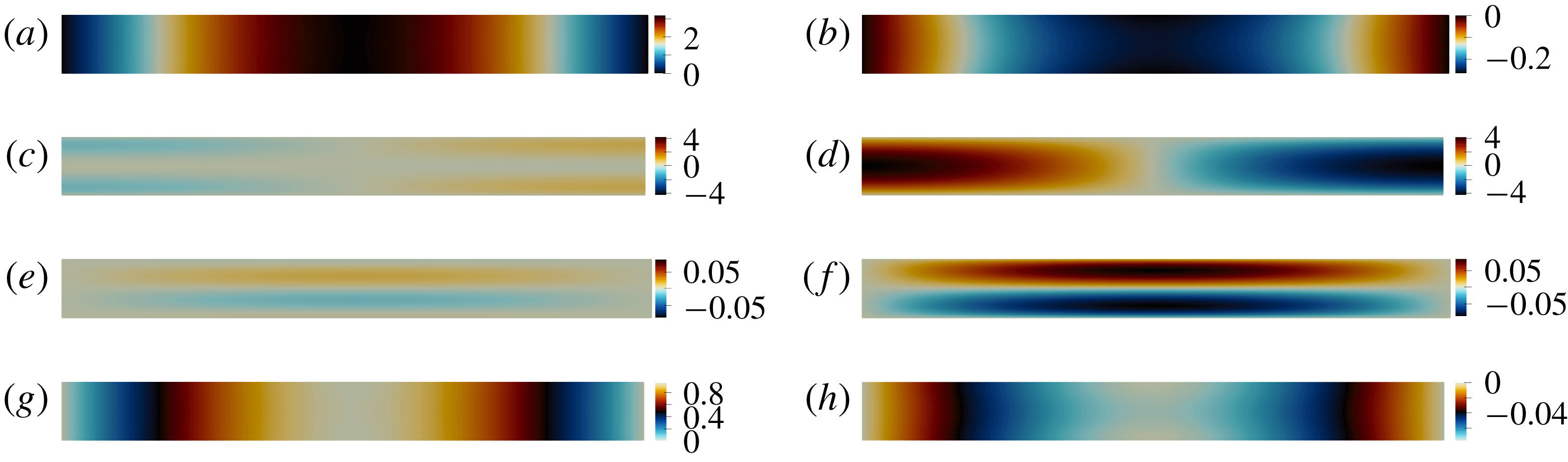
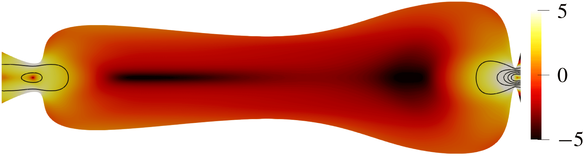
Using the adjoint approach, it is possible to obtain the sensitivity of the objective functions to shape modifications. The shape sensitivity of the steady flow viscous dissipation is calculated using results obtained by Schmidt & Schulz (Reference Schmidt and Schulz2010). In this paper we derive the adjoint counterpart of the thermoviscous acoustic equations and calculate the natural frequency and decay rate shape sensitivities (e.g. Luchini & Bottaro Reference Luchini and Bottaro2014). The gradient-based optimization is then applied to a two-dimensional (2-D) channel and a generic geometry of the printhead’s microchannels. The main goal of this paper is to describe the method that we use and the physics that it exploits. Constraining the channel to be two-dimensional considerably reduces the computational expense of the problem without altering the most influential aspects of the physics. This is because the longest-lasting residual oscillations are those of the lowest frequency mode, whose frequency is determined mainly by the length of the channel and whose dissipation is predominantly in the boundary layers at the sides of the channel. Our 2-D optimization process changes the height of the channel, increasing this dissipation in influential areas. A 3-D process would also change the width of the channel, but we expect this change to be in the same areas, for the same reasons. The 2-D simulations under-estimate the dissipation because they have two sides, rather than four, but they capture the major shape changes required in both the 2-D and 3-D cases. Nevertheless, our next step is to repeat the calculations for a 3-D geometry and with the large number of extra shape parameters that this will entail.
2 Equations of motion in the low Mach number limit
The motion of a fluid with viscosity, heat conductivity, compressibility and external body forces is governed by the compressible Navier–Stokes equations, which, in conservative form, are governed by:
 $$\begin{eqnarray}\frac{\unicode[STIX]{x2202}}{\unicode[STIX]{x2202}t}\boldsymbol{q}+\unicode[STIX]{x1D735}_{k}(\boldsymbol{f}_{k}^{c}(\boldsymbol{q})-\boldsymbol{f}_{k}^{v}(\boldsymbol{q},\unicode[STIX]{x1D735}\boldsymbol{\cdot }\boldsymbol{q}))=0\quad \text{in }\unicode[STIX]{x1D6FA},\end{eqnarray}$$
where
 $\unicode[STIX]{x1D735}_{k}$
is the
$\unicode[STIX]{x1D735}_{k}$
is the
 $k$
th component of the spatial derivative
$k$
th component of the spatial derivative
 $\unicode[STIX]{x1D735}_{k}\equiv \unicode[STIX]{x2202}/\unicode[STIX]{x2202}x_{k}$
, superscripts
$\unicode[STIX]{x1D735}_{k}\equiv \unicode[STIX]{x2202}/\unicode[STIX]{x2202}x_{k}$
, superscripts
 $^{c}$
and
$^{c}$
and
 $^{v}$
refer to convective and viscous components of the equations. The vector of conservative variables,
$^{v}$
refer to convective and viscous components of the equations. The vector of conservative variables,
 $\boldsymbol{q}$
, and the fluxes,
$\boldsymbol{q}$
, and the fluxes,
 $f^{c}(\boldsymbol{q}),f^{v}(\boldsymbol{q})$
, are defined by
$f^{c}(\boldsymbol{q}),f^{v}(\boldsymbol{q})$
, are defined by
 $$\begin{eqnarray}\boldsymbol{q}\equiv \left[\begin{array}{@{}c@{}}\unicode[STIX]{x1D70C}\\ \unicode[STIX]{x1D70C}u_{i}\\ \unicode[STIX]{x1D70C}E\end{array}\right],\quad f_{k}^{c}(\boldsymbol{q})=\left[\begin{array}{@{}c@{}}\unicode[STIX]{x1D70C}u_{k}\\ \unicode[STIX]{x1D70C}u_{i}u_{k}+P\unicode[STIX]{x1D6FF}_{ik}\\ \unicode[STIX]{x1D70C}u_{k}(\unicode[STIX]{x1D70C}E+P)\end{array}\right],\quad f_{k}^{v}(\boldsymbol{q})=\left[\begin{array}{@{}c@{}}0\\ \unicode[STIX]{x1D70F}_{ki}\\ \unicode[STIX]{x1D70F}_{kj}u_{j}+\unicode[STIX]{x1D705}\unicode[STIX]{x1D735}_{k}T\end{array}\right].\end{eqnarray}$$
The variables
 $\unicode[STIX]{x1D70C},\boldsymbol{u},P,T$
denote the flow density, velocity vector, pressure and temperature;
$\unicode[STIX]{x1D70C},\boldsymbol{u},P,T$
denote the flow density, velocity vector, pressure and temperature;
 $\unicode[STIX]{x1D70F}_{ij}$
is the viscous stress tensor, which is proportional to the dynamic viscosity coefficient
$\unicode[STIX]{x1D70F}_{ij}$
is the viscous stress tensor, which is proportional to the dynamic viscosity coefficient
 $\unicode[STIX]{x1D707}_{vis}$
 $$\begin{eqnarray}\unicode[STIX]{x1D70F}_{ij}=\unicode[STIX]{x1D707}_{vis}\left(\unicode[STIX]{x1D735}_{i}u_{j}+\unicode[STIX]{x1D735}_{j}u_{i}-{\textstyle \frac{2}{3}}\unicode[STIX]{x1D6FF}_{ij}\unicode[STIX]{x1D735}_{k}u_{k}\right),\end{eqnarray}$$
and the total energy of the flow
 $E$
is a sum of the kinetic energy and the static internal energy
$E$
is a sum of the kinetic energy and the static internal energy
 $e=e(T,P)$
:
$e=e(T,P)$
:
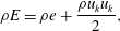 $$\begin{eqnarray}\unicode[STIX]{x1D70C}E=\unicode[STIX]{x1D70C}e+\frac{\unicode[STIX]{x1D70C}u_{k}u_{k}}{2},\end{eqnarray}$$
and
 $\unicode[STIX]{x1D705}$
is the thermal conductivity coefficient. We also introduce an equation of state, which relates the pressure, density and temperature:
$\unicode[STIX]{x1D705}$
is the thermal conductivity coefficient. We also introduce an equation of state, which relates the pressure, density and temperature:
 $$\begin{eqnarray}\unicode[STIX]{x1D70C}=\unicode[STIX]{x1D70C}(P,T).\end{eqnarray}$$
2.1 Low Mach number expansion
Equation (2.1) can describe a range of physical phenomena, which is excessive in this case because the system’s behaviour is governed to first order by only two phenomena. The first is steady flow in a channel with rigid boundaries, with the inlet velocity of order
 $\bar{U}=0.1~\text{m}~\text{s}^{-1}$
and
$\bar{U}=0.1~\text{m}~\text{s}^{-1}$
and
 $Re\approx 1$
. The second is periodic acoustic oscillation, with a small displacement amplitude at the boundary
$Re\approx 1$
. The second is periodic acoustic oscillation, with a small displacement amplitude at the boundary
 $\unicode[STIX]{x1D6E5}\leqslant 0.1~\unicode[STIX]{x03BC}\text{m}$
and a high oscillation frequency
$\unicode[STIX]{x1D6E5}\leqslant 0.1~\unicode[STIX]{x03BC}\text{m}$
and a high oscillation frequency
 $\unicode[STIX]{x1D714}\approx 100~\text{kHz}$
. The characteristic oscillation velocity is of order
$\unicode[STIX]{x1D714}\approx 100~\text{kHz}$
. The characteristic oscillation velocity is of order
 $\tilde{U} =\unicode[STIX]{x1D714}\unicode[STIX]{x1D6E5}\approx 0.01~\text{m}~\text{s}^{-1}$
.
$\tilde{U} =\unicode[STIX]{x1D714}\unicode[STIX]{x1D6E5}\approx 0.01~\text{m}~\text{s}^{-1}$
.
We choose the ambient state density
 $\unicode[STIX]{x1D70C}^{b}$
and the speed of sound
$\unicode[STIX]{x1D70C}^{b}$
and the speed of sound
 $(c_{s}^{b})^{2}=(\unicode[STIX]{x2202}P/\unicode[STIX]{x2202}\unicode[STIX]{x1D70C})_{s}$
as the reference dimensional density and velocity, and the characteristic domain size
$(c_{s}^{b})^{2}=(\unicode[STIX]{x2202}P/\unicode[STIX]{x2202}\unicode[STIX]{x1D70C})_{s}$
as the reference dimensional density and velocity, and the characteristic domain size
 $L$
as the reference length. The reference pressure
$L$
as the reference length. The reference pressure
 $P^{b}$
is chosen as a function of density and the speed of sound:
$P^{b}$
is chosen as a function of density and the speed of sound:
 $P^{b}=\unicode[STIX]{x1D70C}^{b}(c_{s}^{b})^{2}$
, and the reference temperature
$P^{b}=\unicode[STIX]{x1D70C}^{b}(c_{s}^{b})^{2}$
, and the reference temperature
 $T^{b}$
is the ambient temperature.
$T^{b}$
is the ambient temperature.
In this problem, we assume that the local Mach number is small:
 $$\begin{eqnarray}M\equiv \frac{|u|}{c_{s}^{b}}\ll 1.\end{eqnarray}$$
The characteristic velocity amplitudes of the steady flow,
 $\bar{U}$
, and the oscillating flow,
$\bar{U}$
, and the oscillating flow,
 $\tilde{U}$
, are also small in comparison to the speed of sound, which allows us to introduce two small parameters: the steady flow Mach number,
$\tilde{U}$
, are also small in comparison to the speed of sound, which allows us to introduce two small parameters: the steady flow Mach number,
 $\unicode[STIX]{x1D707}$
, and the oscillating flow Mach number,
$\unicode[STIX]{x1D707}$
, and the oscillating flow Mach number,
 $\unicode[STIX]{x1D716}$
:
$\unicode[STIX]{x1D716}$
:
 $$\begin{eqnarray}\displaystyle & \displaystyle \unicode[STIX]{x1D707}\equiv \frac{\bar{U}}{c_{s}^{b}}\simeq \frac{0.1}{1000}\ll 1, & \displaystyle\end{eqnarray}$$
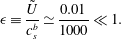 $$\begin{eqnarray}\displaystyle & \displaystyle \unicode[STIX]{x1D716}\equiv \frac{\tilde{U} }{c_{s}^{b}}\simeq \frac{0.01}{1000}\ll 1. & \displaystyle\end{eqnarray}$$
The oscillating flow time scale differs greatly from the steady flow time scale. The oscillating time scale is
 $t_{ac}\sim L/c_{s}$
, and the steady flow time scale is
$t_{ac}\sim L/c_{s}$
, and the steady flow time scale is
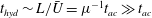 $t_{hyd}\sim L/\bar{U}=\unicode[STIX]{x1D707}^{-1}t_{ac}\gg t_{ac}$
. This allows us to decouple two phenomena and study them independently. We consider a generic state variable
$t_{hyd}\sim L/\bar{U}=\unicode[STIX]{x1D707}^{-1}t_{ac}\gg t_{ac}$
. This allows us to decouple two phenomena and study them independently. We consider a generic state variable
 $\unicode[STIX]{x1D713}(\boldsymbol{x},t)=(\unicode[STIX]{x1D70C},u_{i},P)$
. We denote a zero-order state variable by
$\unicode[STIX]{x1D713}(\boldsymbol{x},t)=(\unicode[STIX]{x1D70C},u_{i},P)$
. We denote a zero-order state variable by
 $\unicode[STIX]{x1D713}_{0}(\boldsymbol{x},t)$
, as if the steady flow and the oscillating flow were absent, i.e.
$\unicode[STIX]{x1D713}_{0}(\boldsymbol{x},t)$
, as if the steady flow and the oscillating flow were absent, i.e.
 $\unicode[STIX]{x1D716}=\unicode[STIX]{x1D707}=0$
. If there is no external energy and momentum production (by imposed temperature gradients, heat release or body forces), then
$\unicode[STIX]{x1D716}=\unicode[STIX]{x1D707}=0$
. If there is no external energy and momentum production (by imposed temperature gradients, heat release or body forces), then
 $\unicode[STIX]{x1D713}_{0}$
is uniform in space and constant in time. We then assume that the perturbation
$\unicode[STIX]{x1D713}_{0}$
is uniform in space and constant in time. We then assume that the perturbation
 $\unicode[STIX]{x1D719}(\boldsymbol{x},t)$
of
$\unicode[STIX]{x1D719}(\boldsymbol{x},t)$
of
 $\unicode[STIX]{x1D713}_{0}$
is at least linearly proportional to
$\unicode[STIX]{x1D713}_{0}$
is at least linearly proportional to
 $\unicode[STIX]{x1D707}$
and
$\unicode[STIX]{x1D707}$
and
 $\unicode[STIX]{x1D716}$
, such that:
$\unicode[STIX]{x1D716}$
, such that:
 $$\begin{eqnarray}\unicode[STIX]{x1D713}(\boldsymbol{x},t)=\unicode[STIX]{x1D713}_{0}+\unicode[STIX]{x1D719}(\boldsymbol{x},t,\unicode[STIX]{x1D707},\unicode[STIX]{x1D716}).\end{eqnarray}$$
We assume that a flow state perturbation related to a particular phenomenon depends solely on the phenomenon’s temporal scale, such that
 $\unicode[STIX]{x1D719}(\boldsymbol{x},t)$
becomes a sum of the slow hydrodynamic perturbation
$\unicode[STIX]{x1D719}(\boldsymbol{x},t)$
becomes a sum of the slow hydrodynamic perturbation
 $\bar{\unicode[STIX]{x1D719}}(\boldsymbol{x},t,\unicode[STIX]{x1D707})$
, labelled the steady flow, and the fast acoustic perturbation
$\bar{\unicode[STIX]{x1D719}}(\boldsymbol{x},t,\unicode[STIX]{x1D707})$
, labelled the steady flow, and the fast acoustic perturbation
 $\tilde{\unicode[STIX]{x1D719}}(\boldsymbol{x},t.\unicode[STIX]{x1D716})$
, labelled the oscillating flow:
$\tilde{\unicode[STIX]{x1D719}}(\boldsymbol{x},t.\unicode[STIX]{x1D716})$
, labelled the oscillating flow:
 $$\begin{eqnarray}\displaystyle & \displaystyle \unicode[STIX]{x1D719}(\boldsymbol{x},t,\unicode[STIX]{x1D707},\unicode[STIX]{x1D716})=\bar{\unicode[STIX]{x1D719}}(\boldsymbol{x},t,\unicode[STIX]{x1D707})+\tilde{\unicode[STIX]{x1D719}}(\boldsymbol{x},t,\unicode[STIX]{x1D716}), & \displaystyle\end{eqnarray}$$
 $$\begin{eqnarray}\displaystyle & \displaystyle \bar{\unicode[STIX]{x1D719}}(\boldsymbol{x},t,\unicode[STIX]{x1D707})=\frac{1}{T_{ac}}\int _{T_{ac}}\unicode[STIX]{x1D719}(\boldsymbol{x},t,\unicode[STIX]{x1D707},\unicode[STIX]{x1D716})\,\text{d}t. & \displaystyle\end{eqnarray}$$
 $\unicode[STIX]{x1D713}(\boldsymbol{x},t)$
consists of the zero-frequency ambient state,
$\unicode[STIX]{x1D713}(\boldsymbol{x},t)$
consists of the zero-frequency ambient state,
 $\unicode[STIX]{x1D713}_{0}$
, the low-frequency hydrodynamic perturbation
$\unicode[STIX]{x1D713}_{0}$
, the low-frequency hydrodynamic perturbation
 $\bar{\unicode[STIX]{x1D719}}(\boldsymbol{x},t_{hyd},\unicode[STIX]{x1D707})$
and the high-frequency acoustic perturbation
$\bar{\unicode[STIX]{x1D719}}(\boldsymbol{x},t_{hyd},\unicode[STIX]{x1D707})$
and the high-frequency acoustic perturbation
 $\tilde{\unicode[STIX]{x1D719}}(\boldsymbol{x},t_{ac},\unicode[STIX]{x1D716})$
:
$\tilde{\unicode[STIX]{x1D719}}(\boldsymbol{x},t_{ac},\unicode[STIX]{x1D716})$
:  $$\begin{eqnarray}\unicode[STIX]{x1D713}(\boldsymbol{x},t)=\unicode[STIX]{x1D713}_{0}+\bar{\unicode[STIX]{x1D719}}(\boldsymbol{x},t_{hyd},\unicode[STIX]{x1D707})+\tilde{\unicode[STIX]{x1D719}}(\boldsymbol{x},t_{ac},\unicode[STIX]{x1D716}).\end{eqnarray}$$
We can perform a low Mach number expansion in terms of
 $\unicode[STIX]{x1D707}$
and
$\unicode[STIX]{x1D707}$
and
 $\unicode[STIX]{x1D716}$
because they are both small. The state perturbations
$\unicode[STIX]{x1D716}$
because they are both small. The state perturbations
 $\bar{\unicode[STIX]{x1D719}}(\boldsymbol{x},t_{hyd})$
and
$\bar{\unicode[STIX]{x1D719}}(\boldsymbol{x},t_{hyd})$
and
 $\tilde{\unicode[STIX]{x1D719}}(\boldsymbol{x},t_{ac})$
independently tend to zero as
$\tilde{\unicode[STIX]{x1D719}}(\boldsymbol{x},t_{ac})$
independently tend to zero as
 $\unicode[STIX]{x1D707}\rightarrow 0$
and
$\unicode[STIX]{x1D707}\rightarrow 0$
and
 $\unicode[STIX]{x1D716}\rightarrow 0$
, so we assume low Mach number decompositions of the form
$\unicode[STIX]{x1D716}\rightarrow 0$
, so we assume low Mach number decompositions of the form
 $\bar{\unicode[STIX]{x1D719}}(\boldsymbol{x},t_{hyd})=\Vert \bar{\unicode[STIX]{x1D719}}\Vert \sum \unicode[STIX]{x1D707}^{k}\bar{\unicode[STIX]{x1D719}}^{(k)}(\boldsymbol{x},t_{hyd})$
and
$\bar{\unicode[STIX]{x1D719}}(\boldsymbol{x},t_{hyd})=\Vert \bar{\unicode[STIX]{x1D719}}\Vert \sum \unicode[STIX]{x1D707}^{k}\bar{\unicode[STIX]{x1D719}}^{(k)}(\boldsymbol{x},t_{hyd})$
and
 $\tilde{\unicode[STIX]{x1D719}}(\boldsymbol{x},t_{ac})=\Vert \tilde{\unicode[STIX]{x1D719}}\Vert \sum \unicode[STIX]{x1D716}^{k}\tilde{\unicode[STIX]{x1D719}}^{(k)}(\boldsymbol{x},t_{ac})$
, where
$\tilde{\unicode[STIX]{x1D719}}(\boldsymbol{x},t_{ac})=\Vert \tilde{\unicode[STIX]{x1D719}}\Vert \sum \unicode[STIX]{x1D716}^{k}\tilde{\unicode[STIX]{x1D719}}^{(k)}(\boldsymbol{x},t_{ac})$
, where
 $\bar{\unicode[STIX]{x1D719}}^{(k)},\tilde{\unicode[STIX]{x1D719}}^{(k)}$
are the
$\bar{\unicode[STIX]{x1D719}}^{(k)},\tilde{\unicode[STIX]{x1D719}}^{(k)}$
are the
 $k$
th-order non-dimensional perturbation shapes, and
$k$
th-order non-dimensional perturbation shapes, and
 $\Vert \bar{\unicode[STIX]{x1D719}}\Vert ,\Vert \tilde{\unicode[STIX]{x1D719}}\Vert$
are the characteristic dimensional magnitudes of the variables:
$\Vert \bar{\unicode[STIX]{x1D719}}\Vert ,\Vert \tilde{\unicode[STIX]{x1D719}}\Vert$
are the characteristic dimensional magnitudes of the variables:
 $\Vert \bar{\unicode[STIX]{x1D70C}}\Vert =\Vert \tilde{\unicode[STIX]{x1D70C}}\Vert =\unicode[STIX]{x1D70C}^{b},\Vert \bar{u}\Vert =\bar{U}$
,
$\Vert \bar{\unicode[STIX]{x1D70C}}\Vert =\Vert \tilde{\unicode[STIX]{x1D70C}}\Vert =\unicode[STIX]{x1D70C}^{b},\Vert \bar{u}\Vert =\bar{U}$
,
 $\Vert \tilde{u} \Vert =\tilde{U}$
,
$\Vert \tilde{u} \Vert =\tilde{U}$
,
 $\Vert \bar{P}\Vert =\Vert \tilde{P}\Vert =P^{b}$
.
$\Vert \bar{P}\Vert =\Vert \tilde{P}\Vert =P^{b}$
.
We neglect the interaction between the steady flow and the oscillating flow given by the higher-order mixed terms
 $\sum \unicode[STIX]{x1D707}^{n}\unicode[STIX]{x1D716}^{m}\unicode[STIX]{x1D719}^{(m+n)}(x,t_{ac},t_{hyd})$
;
$\sum \unicode[STIX]{x1D707}^{n}\unicode[STIX]{x1D716}^{m}\unicode[STIX]{x1D719}^{(m+n)}(x,t_{ac},t_{hyd})$
;
 $m,n\geqslant 1$
because
$m,n\geqslant 1$
because
 $\unicode[STIX]{x1D716}$
and
$\unicode[STIX]{x1D716}$
and
 $\unicode[STIX]{x1D707}$
are both small. The expansion of the primal variables is therefore:
$\unicode[STIX]{x1D707}$
are both small. The expansion of the primal variables is therefore:
 $$\begin{eqnarray}\displaystyle \unicode[STIX]{x1D70C}(x,t) & = & \displaystyle \unicode[STIX]{x1D70C}^{b}\unicode[STIX]{x1D70C}_{0}+\unicode[STIX]{x1D70C}^{b}(\unicode[STIX]{x1D707}\bar{\unicode[STIX]{x1D70C}}^{(1)}+\unicode[STIX]{x1D716}\tilde{\unicode[STIX]{x1D70C}}^{(1)})+\mathit{O}(\unicode[STIX]{x1D707}^{2},\unicode[STIX]{x1D716}^{2},\unicode[STIX]{x1D707}\unicode[STIX]{x1D716}),\end{eqnarray}$$
 $$\begin{eqnarray}\displaystyle u(x,t) & = & \displaystyle c_{s}^{b}(\unicode[STIX]{x1D707}\bar{u}^{(1)}+\unicode[STIX]{x1D716}\tilde{u} ^{(1)})+\mathit{O}(\unicode[STIX]{x1D707}^{2},\unicode[STIX]{x1D716}^{2},\unicode[STIX]{x1D707}\unicode[STIX]{x1D716}),\end{eqnarray}$$
 $$\begin{eqnarray}\displaystyle P(x,t) & = & \displaystyle P^{b}P_{0}+P^{b}(\unicode[STIX]{x1D707}\bar{P}^{(1)}+\unicode[STIX]{x1D707}^{2}\bar{P}^{(2)}+\unicode[STIX]{x1D716}\tilde{P}^{(1)})+\mathit{O}(\unicode[STIX]{x1D707}^{3},\unicode[STIX]{x1D716}^{2},\unicode[STIX]{x1D707}\unicode[STIX]{x1D716}).\end{eqnarray}$$
 $\unicode[STIX]{x1D707}^{2}\bar{P}^{(2)}$
here because the first-order steady flow pressure perturbation
$\unicode[STIX]{x1D707}^{2}\bar{P}^{(2)}$
here because the first-order steady flow pressure perturbation
 $\bar{P}^{(1)}$
does not contribute to the steady flow, being a part of the ambient state, as shown by Müller (Reference Müller1998).
$\bar{P}^{(1)}$
does not contribute to the steady flow, being a part of the ambient state, as shown by Müller (Reference Müller1998).2.2 Zero Mach number limit
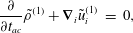
Substituting the primal variables expansion (2.11) into (2.1) and (2.5), and collecting the zero-order terms, we obtain:
 $$\begin{eqnarray}\displaystyle & \displaystyle \unicode[STIX]{x1D735}_{i}P^{(0)}(x)=0, & \displaystyle\end{eqnarray}$$
 $$\begin{eqnarray}\displaystyle & \displaystyle \unicode[STIX]{x1D735}_{k}(\unicode[STIX]{x1D705}\unicode[STIX]{x1D735}_{k}T^{(0)}(x))=0, & \displaystyle\end{eqnarray}$$
 $$\begin{eqnarray}\displaystyle & \displaystyle \unicode[STIX]{x1D70C}^{(0)}(x)=\unicode[STIX]{x1D70C}(P^{(0)},T^{(0)}). & \displaystyle\end{eqnarray}$$
The zeroth-order equations describe the ambient state,
 $\unicode[STIX]{x1D716}=\unicode[STIX]{x1D707}=0$
. Equation (2.12a
) shows that the ambient pressure
$\unicode[STIX]{x1D716}=\unicode[STIX]{x1D707}=0$
. Equation (2.12a
) shows that the ambient pressure
 $P_{0}$
is spatially uniform, and (2.12b
) describes the temperature distribution of the ambient state. If all the boundaries have uniform and constant temperature, then the ambient temperature and density are uniform and non-dimensionalized as
$P_{0}$
is spatially uniform, and (2.12b
) describes the temperature distribution of the ambient state. If all the boundaries have uniform and constant temperature, then the ambient temperature and density are uniform and non-dimensionalized as
 $T^{(0)}(x)=1,\unicode[STIX]{x1D70C}^{(0)}(x)=1$
.
$T^{(0)}(x)=1,\unicode[STIX]{x1D70C}^{(0)}(x)=1$
.
2.3 Low Mach number steady flow
Collecting the first-order terms of
 $\unicode[STIX]{x1D707}$
in the continuity equation and the second-order terms of
$\unicode[STIX]{x1D707}$
in the continuity equation and the second-order terms of
 $\unicode[STIX]{x1D707}^{2}$
in the momentum equations (2.2) and assuming a Newtonian fluid results in the incompressible Navier–Stokes equation:
$\unicode[STIX]{x1D707}^{2}$
in the momentum equations (2.2) and assuming a Newtonian fluid results in the incompressible Navier–Stokes equation:
 $$\begin{eqnarray}\displaystyle & \displaystyle \unicode[STIX]{x1D735}_{i}\bar{u}_{i}^{(1)}=0, & \displaystyle\end{eqnarray}$$
 $$\begin{eqnarray}\displaystyle & \displaystyle \frac{\unicode[STIX]{x2202}}{\unicode[STIX]{x2202}t_{hyd}}\bar{u}_{i}^{(1)}+(\bar{u}_{j}^{(1)}\unicode[STIX]{x1D735}_{j})\bar{u}_{i}^{(1)}+\unicode[STIX]{x1D735}_{i}\bar{P}^{(2)}-\frac{1}{\overline{Re}}\unicode[STIX]{x0394}\bar{u}_{i}^{(1)}=0. & \displaystyle\end{eqnarray}$$
 $\bar{P}$
, balances the nonlinear convective term in the momentum equation, so
$\bar{P}$
, balances the nonlinear convective term in the momentum equation, so
 $\bar{P}=\unicode[STIX]{x1D707}^{2}\bar{P}^{(2)}+\mathit{O}(\unicode[STIX]{x1D707}^{3})$
. Here
$\bar{P}=\unicode[STIX]{x1D707}^{2}\bar{P}^{(2)}+\mathit{O}(\unicode[STIX]{x1D707}^{3})$
. Here
 $\overline{Re}\equiv \unicode[STIX]{x1D70C}^{b}LU_{in}/\unicode[STIX]{x1D707}_{vis}$
is the steady flow Reynolds number.
$\overline{Re}\equiv \unicode[STIX]{x1D70C}^{b}LU_{in}/\unicode[STIX]{x1D707}_{vis}$
is the steady flow Reynolds number. We supplement the steady flow equations with a prescribed velocity boundary condition at the inlet,
 $\unicode[STIX]{x1D6E4}_{in}$
, a no-slip boundary condition on the walls,
$\unicode[STIX]{x1D6E4}_{in}$
, a no-slip boundary condition on the walls,
 $\unicode[STIX]{x1D6E4}_{w}$
, and a zero stress boundary condition at the outlet,
$\unicode[STIX]{x1D6E4}_{w}$
, and a zero stress boundary condition at the outlet,
 $\unicode[STIX]{x1D6E4}_{out}$
:
$\unicode[STIX]{x1D6E4}_{out}$
:
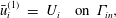 $$\begin{eqnarray}\displaystyle \bar{u}_{i}^{(1)} & = & \displaystyle U_{i}\quad \text{on }\unicode[STIX]{x1D6E4}_{in},\end{eqnarray}$$
 $$\begin{eqnarray}\displaystyle \bar{u}_{i}^{(1)} & = & \displaystyle 0\quad \text{on }\unicode[STIX]{x1D6E4}_{w},\end{eqnarray}$$
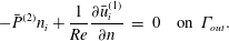 $$\begin{eqnarray}\displaystyle -\bar{P}^{(2)}n_{i}+\frac{1}{Re}\frac{\unicode[STIX]{x2202}\bar{u}_{i}^{(1)}}{\unicode[STIX]{x2202}n} & = & \displaystyle 0\quad \text{on }\unicode[STIX]{x1D6E4}_{out}.\end{eqnarray}$$
2.4 Low Mach number oscillating flow
Collecting the first-order terms of
 $\unicode[STIX]{x1D716}$
, the oscillating flow continuity, momentum and energy equations are governed by:
$\unicode[STIX]{x1D716}$
, the oscillating flow continuity, momentum and energy equations are governed by:
 $$\begin{eqnarray}\displaystyle \frac{\unicode[STIX]{x2202}}{\unicode[STIX]{x2202}t_{ac}}\tilde{\unicode[STIX]{x1D70C}}^{(1)}+\unicode[STIX]{x1D735}_{i}\tilde{u} _{i}^{(1)} & = & \displaystyle 0,\end{eqnarray}$$
 $$\begin{eqnarray}\displaystyle \frac{\unicode[STIX]{x2202}}{\unicode[STIX]{x2202}t_{ac}}\tilde{u} _{i}^{(1)}+\unicode[STIX]{x1D735}_{i}\tilde{P}^{(1)} & = & \displaystyle \frac{1}{\tilde{Re}}\unicode[STIX]{x1D735}_{j}\tilde{\unicode[STIX]{x1D70F}}_{ij}^{(1)},\end{eqnarray}$$
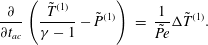
 $$\begin{eqnarray}\displaystyle \frac{s^{b}}{c_{p}}\frac{\unicode[STIX]{x2202}}{\unicode[STIX]{x2202}t_{ac}}\tilde{s}^{(1)} & = & \displaystyle \frac{1}{\tilde{Pe}}\unicode[STIX]{x0394}\tilde{T}^{(1)}.\end{eqnarray}$$
The Reynolds and Péclet numbers based on the speed of sound are
 $\tilde{Re}\equiv \unicode[STIX]{x1D70C}^{b}Lc_{s}^{b}/\unicode[STIX]{x1D707}_{vis}$
and
$\tilde{Re}\equiv \unicode[STIX]{x1D70C}^{b}Lc_{s}^{b}/\unicode[STIX]{x1D707}_{vis}$
and
 $\tilde{Pe}\equiv \unicode[STIX]{x1D70C}^{b}Lc_{s}^{b}c_{p}/\unicode[STIX]{x1D705}$
. The heat capacity ratio is
$\tilde{Pe}\equiv \unicode[STIX]{x1D70C}^{b}Lc_{s}^{b}c_{p}/\unicode[STIX]{x1D705}$
. The heat capacity ratio is
 $\unicode[STIX]{x1D6FE}\equiv c_{p}/c_{v}$
, where
$\unicode[STIX]{x1D6FE}\equiv c_{p}/c_{v}$
, where
 $c_{p}$
and
$c_{p}$
and
 $c_{v}$
are the specific heats at constant pressure and constant volume, and
$c_{v}$
are the specific heats at constant pressure and constant volume, and
 $s^{b}$
is the dimensional ambient state entropy. The viscous contribution to the mechanical energy dissipation
$s^{b}$
is the dimensional ambient state entropy. The viscous contribution to the mechanical energy dissipation
 $\unicode[STIX]{x1D735}_{k}(\tilde{\unicode[STIX]{x1D70F}}_{kj}^{(1)}\tilde{u} _{j}^{(1)})$
is absent in (2.15c
) because it is second order in
$\unicode[STIX]{x1D735}_{k}(\tilde{\unicode[STIX]{x1D70F}}_{kj}^{(1)}\tilde{u} _{j}^{(1)})$
is absent in (2.15c
) because it is second order in
 $\unicode[STIX]{x1D716}$
and therefore negligible. We solve the oscillating flow equations in terms of the oscillating flow pressure
$\unicode[STIX]{x1D716}$
and therefore negligible. We solve the oscillating flow equations in terms of the oscillating flow pressure
 $\tilde{P}^{(1)}$
, velocity
$\tilde{P}^{(1)}$
, velocity
 $\tilde{u} _{i}^{(1)}$
and temperature
$\tilde{u} _{i}^{(1)}$
and temperature
 $\tilde{T}^{(1)}$
, and express the flow density and entropy as
$\tilde{T}^{(1)}$
, and express the flow density and entropy as
 $\tilde{s}^{(1)}=\tilde{s}(\tilde{P}^{(1)},\tilde{T}^{(1)})$
, and
$\tilde{s}^{(1)}=\tilde{s}(\tilde{P}^{(1)},\tilde{T}^{(1)})$
, and
 $\tilde{\unicode[STIX]{x1D70C}}^{(1)}=\tilde{\unicode[STIX]{x1D70C}}(\tilde{P}^{(1)},\tilde{T}^{(1)})$
using the following thermodynamic equalities:
$\tilde{\unicode[STIX]{x1D70C}}^{(1)}=\tilde{\unicode[STIX]{x1D70C}}(\tilde{P}^{(1)},\tilde{T}^{(1)})$
using the following thermodynamic equalities:
 $$\begin{eqnarray}\displaystyle & \displaystyle s^{b}\tilde{s}^{(1)}=\left(\frac{\unicode[STIX]{x2202}S}{\unicode[STIX]{x2202}P}\right)_{T}P^{b}\tilde{P}^{(1)}+\left(\frac{\unicode[STIX]{x2202}S}{\unicode[STIX]{x2202}T}\right)_{P}T^{b}\tilde{T}^{(1)}=-\frac{\unicode[STIX]{x1D6FC}_{p}}{\unicode[STIX]{x1D70C}_{b}}P^{b}\tilde{P}^{(1)}+\frac{c_{p}}{T_{b}}T^{b}\tilde{T}^{(1)}, & \displaystyle\end{eqnarray}$$
 $$\begin{eqnarray}\displaystyle & \displaystyle \unicode[STIX]{x1D70C}^{b}\tilde{\unicode[STIX]{x1D70C}}^{(1)}=\left(\frac{\unicode[STIX]{x2202}\unicode[STIX]{x1D70C}}{\unicode[STIX]{x2202}P}\right)_{T}P^{b}\tilde{P}^{(1)}+\left(\frac{\unicode[STIX]{x2202}\unicode[STIX]{x1D70C}}{\unicode[STIX]{x2202}T}\right)_{P}T^{b}\tilde{T}^{(1)}=\frac{\unicode[STIX]{x1D6FE}}{(c_{s}^{b})^{2}}P^{b}\tilde{P}^{(1)}-\unicode[STIX]{x1D70C}^{b}\unicode[STIX]{x1D6FC}_{p}T^{b}\tilde{T}^{(1)}, & \displaystyle\end{eqnarray}$$
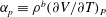 $\unicode[STIX]{x1D6FC}_{p}\equiv \unicode[STIX]{x1D70C}^{b}(\unicode[STIX]{x2202}V/\unicode[STIX]{x2202}T)_{P}$
is the volumetric coefficient of thermal expansion. These expressions are substituted into (2.15). For convenience, we redefine the oscillating flow temperature as
$\unicode[STIX]{x1D6FC}_{p}\equiv \unicode[STIX]{x1D70C}^{b}(\unicode[STIX]{x2202}V/\unicode[STIX]{x2202}T)_{P}$
is the volumetric coefficient of thermal expansion. These expressions are substituted into (2.15). For convenience, we redefine the oscillating flow temperature as
 $\unicode[STIX]{x1D6FC}_{p}T^{b}\tilde{T}^{(1)}\rightarrow \tilde{T}^{(1)}$
, and use the fact that
$\unicode[STIX]{x1D6FC}_{p}T^{b}\tilde{T}^{(1)}\rightarrow \tilde{T}^{(1)}$
, and use the fact that
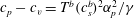 $c_{p}-c_{v}=T^{b}(c_{s}^{b})^{2}\unicode[STIX]{x1D6FC}_{p}^{2}/\unicode[STIX]{x1D6FE}$
to express the continuity (2.15a
) and energy (2.15c
) equations in terms of pressure and temperature:
$c_{p}-c_{v}=T^{b}(c_{s}^{b})^{2}\unicode[STIX]{x1D6FC}_{p}^{2}/\unicode[STIX]{x1D6FE}$
to express the continuity (2.15a
) and energy (2.15c
) equations in terms of pressure and temperature: 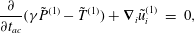 $$\begin{eqnarray}\displaystyle \frac{\unicode[STIX]{x2202}}{\unicode[STIX]{x2202}t_{ac}}(\unicode[STIX]{x1D6FE}\tilde{P}^{(1)}-\tilde{T}^{(1)})+\unicode[STIX]{x1D735}_{i}\tilde{u} _{i}^{(1)} & = & \displaystyle 0,\end{eqnarray}$$
 $$\begin{eqnarray}\displaystyle \frac{\unicode[STIX]{x2202}}{\unicode[STIX]{x2202}t_{ac}}\left(\frac{\tilde{T}^{(1)}}{\unicode[STIX]{x1D6FE}-1}-\tilde{P}^{(1)}\right) & = & \displaystyle \frac{1}{\tilde{Pe}}\unicode[STIX]{x0394}\tilde{T}^{(1)}.\end{eqnarray}$$
 $$\begin{eqnarray}\tilde{\unicode[STIX]{x1D70C}}^{(1)}\equiv \unicode[STIX]{x1D6FE}\tilde{P}^{(1)}-\tilde{T}^{(1)},\quad \tilde{s}^{(1)}\equiv \frac{\tilde{T}^{(1)}}{\unicode[STIX]{x1D6FE}-1}-\tilde{P}^{(1)}.\end{eqnarray}$$
No-slip velocity
 $\tilde{u} ^{(1)}=0$
and isothermal
$\tilde{u} ^{(1)}=0$
and isothermal
 $\tilde{T}^{(1)}=0$
boundary conditions induce viscous and thermal boundary layers, which damp the acoustic waves. The thickness of the viscous boundary layer
$\tilde{T}^{(1)}=0$
boundary conditions induce viscous and thermal boundary layers, which damp the acoustic waves. The thickness of the viscous boundary layer
 $\unicode[STIX]{x1D6FF}_{\unicode[STIX]{x1D708}}$
and the thermal boundary layer
$\unicode[STIX]{x1D6FF}_{\unicode[STIX]{x1D708}}$
and the thermal boundary layer
 $\unicode[STIX]{x1D6FF}_{T}$
depends on the oscillation frequency (Beltman Reference Beltman1999):
$\unicode[STIX]{x1D6FF}_{T}$
depends on the oscillation frequency (Beltman Reference Beltman1999):
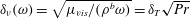 $\unicode[STIX]{x1D6FF}_{\unicode[STIX]{x1D708}}(\unicode[STIX]{x1D714})=\sqrt{\unicode[STIX]{x1D707}_{vis}/(\unicode[STIX]{x1D70C}^{b}\unicode[STIX]{x1D714})}=\unicode[STIX]{x1D6FF}_{T}\sqrt{Pr}$
. The non-dimensional viscous and thermal boundary layers thicknesses,
$\unicode[STIX]{x1D6FF}_{\unicode[STIX]{x1D708}}(\unicode[STIX]{x1D714})=\sqrt{\unicode[STIX]{x1D707}_{vis}/(\unicode[STIX]{x1D70C}^{b}\unicode[STIX]{x1D714})}=\unicode[STIX]{x1D6FF}_{T}\sqrt{Pr}$
. The non-dimensional viscous and thermal boundary layers thicknesses,
 $\tilde{\unicode[STIX]{x1D6FF}}_{\unicode[STIX]{x1D708}}(\unicode[STIX]{x1D714}),\tilde{\unicode[STIX]{x1D6FF}}_{T}(\unicode[STIX]{x1D714})$
, are:
$\tilde{\unicode[STIX]{x1D6FF}}_{\unicode[STIX]{x1D708}}(\unicode[STIX]{x1D714}),\tilde{\unicode[STIX]{x1D6FF}}_{T}(\unicode[STIX]{x1D714})$
, are:
 $$\begin{eqnarray}\tilde{\unicode[STIX]{x1D6FF}}_{\unicode[STIX]{x1D708}}^{2}(\unicode[STIX]{x1D714})=\frac{\unicode[STIX]{x1D6FF}_{\unicode[STIX]{x1D708}}^{2}(\unicode[STIX]{x1D714})}{L^{2}}=\frac{1}{\tilde{Re}}\frac{\unicode[STIX]{x1D714}_{ac}}{\unicode[STIX]{x1D714}},\quad \tilde{\unicode[STIX]{x1D6FF}}_{T}^{2}(\unicode[STIX]{x1D714})=\frac{\unicode[STIX]{x1D6FF}_{T}^{2}(\unicode[STIX]{x1D714})}{L^{2}}=\frac{1}{\tilde{Pe}}\frac{\unicode[STIX]{x1D714}_{ac}}{\unicode[STIX]{x1D714}},\end{eqnarray}$$
where
 $\unicode[STIX]{x1D714}_{ac}=t_{ac}^{-1}$
is the characteristic acoustic frequency. If the oscillation frequency,
$\unicode[STIX]{x1D714}_{ac}=t_{ac}^{-1}$
is the characteristic acoustic frequency. If the oscillation frequency,
 $\unicode[STIX]{x1D714}$
, is similar to or smaller than the acoustic frequency,
$\unicode[STIX]{x1D714}$
, is similar to or smaller than the acoustic frequency,
 $\unicode[STIX]{x1D714}_{ac}$
, then the viscothermal effects cannot be ignored for general
$\unicode[STIX]{x1D714}_{ac}$
, then the viscothermal effects cannot be ignored for general
 $\tilde{Re},\tilde{Pe}$
. For an inkjet printhead, the fluid viscosity is of order
$\tilde{Re},\tilde{Pe}$
. For an inkjet printhead, the fluid viscosity is of order
 $10^{-2}~\text{Pa}~\text{s}$
, the speed of sound is
$10^{-2}~\text{Pa}~\text{s}$
, the speed of sound is
 $10^{3}~\text{ms}^{-1}$
and the channel width is of order
$10^{3}~\text{ms}^{-1}$
and the channel width is of order
 $100~\unicode[STIX]{x03BC}\text{m}$
, which results in
$100~\unicode[STIX]{x03BC}\text{m}$
, which results in
 $\unicode[STIX]{x1D714}_{ac}=10~\text{MHz}$
. At the typical operational frequency of
$\unicode[STIX]{x1D714}_{ac}=10~\text{MHz}$
. At the typical operational frequency of
 $\unicode[STIX]{x1D714}=100~\text{kHz}$
the viscous boundary-layer thickness is then
$\unicode[STIX]{x1D714}=100~\text{kHz}$
the viscous boundary-layer thickness is then
 $\tilde{\unicode[STIX]{x1D6FF}}_{\unicode[STIX]{x1D708}}\sim 0.1$
. The thermal boundary layer thickness is smaller by a factor of
$\tilde{\unicode[STIX]{x1D6FF}}_{\unicode[STIX]{x1D708}}\sim 0.1$
. The thermal boundary layer thickness is smaller by a factor of
 $\sqrt{Pr}$
. For inks used in inkjet printers, with
$\sqrt{Pr}$
. For inks used in inkjet printers, with
 $10<Pr<30$
(Seccombe et al.
Reference Seccombe1997)
$10<Pr<30$
(Seccombe et al.
Reference Seccombe1997)
 $\tilde{\unicode[STIX]{x1D6FF}}_{T}\sim 0.025$
.
$\tilde{\unicode[STIX]{x1D6FF}}_{T}\sim 0.025$
.
We perform a modal decomposition of the oscillating flow state vector
 $\tilde{\boldsymbol{q}}(x,t)=\hat{\boldsymbol{q}}(x)\text{e}^{st}$
. The Laplace transform of (2.15) results in an eigenvalue problem
$\tilde{\boldsymbol{q}}(x,t)=\hat{\boldsymbol{q}}(x)\text{e}^{st}$
. The Laplace transform of (2.15) results in an eigenvalue problem
 $sB\hat{\boldsymbol{q}}+A\hat{\boldsymbol{q}}=0$
in terms of
$sB\hat{\boldsymbol{q}}+A\hat{\boldsymbol{q}}=0$
in terms of
 $\hat{\boldsymbol{q}}=(\hat{u} _{i},\hat{P},\hat{T})$
, where
$\hat{\boldsymbol{q}}=(\hat{u} _{i},\hat{P},\hat{T})$
, where
 $\hat{\boldsymbol{q}}$
is the complex eigenfunction, and
$\hat{\boldsymbol{q}}$
is the complex eigenfunction, and
 $s$
is the complex eigenvalue:
$s$
is the complex eigenvalue:
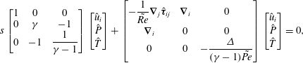 $$\begin{eqnarray}\displaystyle & \displaystyle s\left[\begin{array}{@{}ccc@{}}1 & 0 & 0\\ 0 & \unicode[STIX]{x1D6FE} & -1\\ 0 & -1 & {\displaystyle \frac{1}{\unicode[STIX]{x1D6FE}-1}}\end{array}\right]\left[\begin{array}{@{}c@{}}\hat{u} _{i}\\ \hat{P}\\ \hat{T}\end{array}\right]+\left[\begin{array}{@{}ccc@{}}-{\displaystyle \frac{1}{\tilde{Re}}}\unicode[STIX]{x1D735}_{j}\hat{\unicode[STIX]{x1D749}}_{ij} & \unicode[STIX]{x1D735}_{i} & 0\\ \unicode[STIX]{x1D735}_{i} & 0 & 0\\ 0 & 0 & -{\displaystyle \frac{\unicode[STIX]{x1D6E5}}{(\unicode[STIX]{x1D6FE}-1)\tilde{Pe}}}\end{array}\right]\left[\begin{array}{@{}c@{}}\hat{u} _{i}\\ \hat{P}\\ \hat{T}\end{array}\right]=0,\qquad & \displaystyle\end{eqnarray}$$
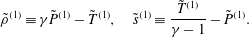
 $$\begin{eqnarray}\displaystyle & \displaystyle s=\unicode[STIX]{x1D70E}+\text{i}\unicode[STIX]{x1D714}, & \displaystyle\end{eqnarray}$$
 $-\unicode[STIX]{x1D70E}$
is the decay rate and
$-\unicode[STIX]{x1D70E}$
is the decay rate and
 $\unicode[STIX]{x1D714}$
is the angular frequency of the mode. The matrix form of the governing equation for the oscillating flow written in this particular form is Hermitian:
$\unicode[STIX]{x1D714}$
is the angular frequency of the mode. The matrix form of the governing equation for the oscillating flow written in this particular form is Hermitian:
 $B=B^{H},A=A^{H}$
.
$B=B^{H},A=A^{H}$
.2.4.1 Boundary conditions
For rigid boundaries we apply a no-slip boundary condition and for open boundaries we apply a stress-free boundary condition:
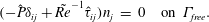
 $$\begin{eqnarray}\displaystyle \hat{u} _{i} & = & \displaystyle 0\quad \text{on }\unicode[STIX]{x1D6E4}_{nsl},\end{eqnarray}$$
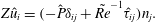
 $$\begin{eqnarray}\displaystyle (-\hat{P}\unicode[STIX]{x1D6FF}_{ij}+\tilde{Re}^{-1}\hat{\unicode[STIX]{x1D70F}}_{ij})n_{j} & = & \displaystyle 0\quad \text{on }\unicode[STIX]{x1D6E4}_{free}.\end{eqnarray}$$
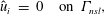
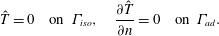 $$\begin{eqnarray}\hat{T}=0\quad \text{on }\unicode[STIX]{x1D6E4}_{iso},\quad \frac{\unicode[STIX]{x2202}\hat{T}}{\unicode[STIX]{x2202}n}=0\quad \text{on }\unicode[STIX]{x1D6E4}_{ad}.\end{eqnarray}$$
If the boundaries are not rigid, they displace in reaction to the flow on the boundary. For inviscid flow, the boundary impedance,
 $Z$
, links the pressure to the velocity on the boundary (Myers Reference Myers1980).
$Z$
, links the pressure to the velocity on the boundary (Myers Reference Myers1980).
 $Z$
is typically frequency dependent:
$Z$
is typically frequency dependent:
 $Z=Z(s)$
. For viscous flow, the force at the boundary needs to include the viscous stress, such that the impedance boundary condition is
$Z=Z(s)$
. For viscous flow, the force at the boundary needs to include the viscous stress, such that the impedance boundary condition is
 $$\begin{eqnarray}Z\hat{u} _{i}=(-\hat{P}\unicode[STIX]{x1D6FF}_{ij}+\tilde{Re}^{-1}\hat{\unicode[STIX]{x1D70F}}_{ij})n_{j}.\end{eqnarray}$$
Here we neither restrict the tangential velocity to be zero nor forbid tangential displacements of the compliant boundary. As
 $Z\rightarrow 0$
, the boundary becomes a free surface,
$Z\rightarrow 0$
, the boundary becomes a free surface,
 $\hat{\unicode[STIX]{x1D70E}}_{ij}n_{j}\rightarrow 0$
. As
$\hat{\unicode[STIX]{x1D70E}}_{ij}n_{j}\rightarrow 0$
. As
 $Z\rightarrow \infty$
, the boundary becomes a no-slip rigid wall,
$Z\rightarrow \infty$
, the boundary becomes a no-slip rigid wall,
 $\hat{u} _{i}\rightarrow 0$
.
$\hat{u} _{i}\rightarrow 0$
.
Similarly, the thermal accommodation coefficient
 $\unicode[STIX]{x1D6FC}_{w}\geqslant 0$
can be introduced to describe the temperature boundary condition (Carslaw & Jaeger Reference Carslaw and Jaeger1986; Beltman Reference Beltman1999),
$\unicode[STIX]{x1D6FC}_{w}\geqslant 0$
can be introduced to describe the temperature boundary condition (Carslaw & Jaeger Reference Carslaw and Jaeger1986; Beltman Reference Beltman1999),
 $$\begin{eqnarray}\hat{T}=-\unicode[STIX]{x1D6FC}_{w}\frac{\unicode[STIX]{x2202}\hat{T}}{\unicode[STIX]{x2202}n}.\end{eqnarray}$$
As
 $\unicode[STIX]{x1D6FC}_{w}\rightarrow 0$
, the boundary becomes isothermal. As
$\unicode[STIX]{x1D6FC}_{w}\rightarrow 0$
, the boundary becomes isothermal. As
 $\unicode[STIX]{x1D6FC}_{w}\rightarrow \infty$
, the boundary becomes adiabatic.
$\unicode[STIX]{x1D6FC}_{w}\rightarrow \infty$
, the boundary becomes adiabatic.
The domain boundaries can have non-uniform compliance and thermal properties. The boundary impedance and thermal accommodation coefficients are non-uniform frequency-dependent functions,
 $Z=Z(s),\unicode[STIX]{x1D6FC}_{w}=\unicode[STIX]{x1D6FC}_{w}(s)$
on
$Z=Z(s),\unicode[STIX]{x1D6FC}_{w}=\unicode[STIX]{x1D6FC}_{w}(s)$
on
 $\unicode[STIX]{x2202}\unicode[STIX]{x1D6FA}$
. In summary, the velocity and temperature boundary conditions can be generalized to Robin boundary conditions (2.23), (2.24), with special cases for rigid and open boundaries:
$\unicode[STIX]{x2202}\unicode[STIX]{x1D6FA}$
. In summary, the velocity and temperature boundary conditions can be generalized to Robin boundary conditions (2.23), (2.24), with special cases for rigid and open boundaries:
 $$\begin{eqnarray}Z=0\quad \text{on }\unicode[STIX]{x1D6E4}_{nsl},\quad Z^{-1}=0\quad \text{on }\unicode[STIX]{x1D6E4}_{free},\end{eqnarray}$$
 $$\begin{eqnarray}\unicode[STIX]{x1D6FC}_{w}=0\quad \text{on }\unicode[STIX]{x1D6E4}_{iso},\quad \unicode[STIX]{x1D6FC}_{w}^{-1}=0\quad \text{on }\unicode[STIX]{x1D6E4}_{ad}.\end{eqnarray}$$
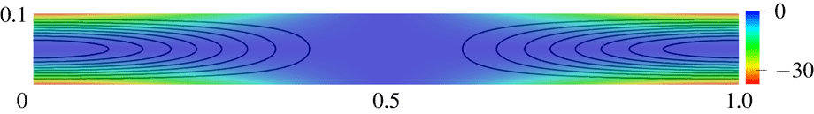
2.4.2 Energy of the acoustic oscillation
The thermoviscous acoustic problem (2.15) is dissipative, and later we will investigate how and where this dissipation occurs. For this we introduce an energy norm (Chu Reference Chu1965),
 $\hat{E}$
, where
$\hat{E}$
, where
 $^{\ast }$
denotes the complex conjugate:
$^{\ast }$
denotes the complex conjugate:
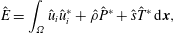 $$\begin{eqnarray}\hat{E}=\int _{\unicode[STIX]{x1D6FA}}\hat{u} _{i}\hat{u} _{i}^{\ast }+\hat{\unicode[STIX]{x1D70C}}\hat{P}^{\ast }+{\hat{s}}\hat{T}^{\ast }\,\text{d}\boldsymbol{x},\end{eqnarray}$$
such that the total energy
 $\tilde{E}=\hat{E}\text{e}^{2st}$
decays in time as
$\tilde{E}=\hat{E}\text{e}^{2st}$
decays in time as
 $\text{e}^{2\unicode[STIX]{x1D70E}t}$
(2.20b
). We premultiply the oscillating flow governing equation (2.20) by the state vector
$\text{e}^{2\unicode[STIX]{x1D70E}t}$
(2.20b
). We premultiply the oscillating flow governing equation (2.20) by the state vector
 $\hat{\boldsymbol{q}}^{\text{T}}$
and integrate it over the volume,
$\hat{\boldsymbol{q}}^{\text{T}}$
and integrate it over the volume,
 $\int _{\unicode[STIX]{x1D6FA}}s\hat{\boldsymbol{q}}^{\text{T}}B\hat{\boldsymbol{q}}+\hat{\boldsymbol{q}}^{\text{T}}A\hat{\boldsymbol{q}}=0$
. We integrate the second term by parts once and apply the boundary conditions (2.23), (2.24). The first term is the energy norm,
$\int _{\unicode[STIX]{x1D6FA}}s\hat{\boldsymbol{q}}^{\text{T}}B\hat{\boldsymbol{q}}+\hat{\boldsymbol{q}}^{\text{T}}A\hat{\boldsymbol{q}}=0$
. We integrate the second term by parts once and apply the boundary conditions (2.23), (2.24). The first term is the energy norm,
 $\int _{\unicode[STIX]{x1D6FA}}\hat{\boldsymbol{q}}^{\text{T}}B\hat{\boldsymbol{q}}=\hat{E}$
, and the second term is the energy dissipation inside the domain and the energy flux through the boundary. We take the real part of this volume integral to express the decay rate of the mode as the sum of volumetric energy dissipation
$\int _{\unicode[STIX]{x1D6FA}}\hat{\boldsymbol{q}}^{\text{T}}B\hat{\boldsymbol{q}}=\hat{E}$
, and the second term is the energy dissipation inside the domain and the energy flux through the boundary. We take the real part of this volume integral to express the decay rate of the mode as the sum of volumetric energy dissipation
 $\unicode[STIX]{x1D70E}_{\unicode[STIX]{x1D6FA}}$
and the surface energy transfer
$\unicode[STIX]{x1D70E}_{\unicode[STIX]{x1D6FA}}$
and the surface energy transfer
 $\unicode[STIX]{x1D70E}_{\unicode[STIX]{x2202}\unicode[STIX]{x1D6FA}}$
:
$\unicode[STIX]{x1D70E}_{\unicode[STIX]{x2202}\unicode[STIX]{x1D6FA}}$
:
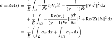 $$\begin{eqnarray}\displaystyle \unicode[STIX]{x1D70E}\equiv \text{Re}(s) & = & \displaystyle \frac{1}{\hat{E}}\int _{\unicode[STIX]{x1D6FA}}-\frac{1}{\tilde{Re}}\hat{\unicode[STIX]{x1D70F}}_{ij}\unicode[STIX]{x1D735}_{j}\hat{u} _{i}^{\ast }-\frac{1}{(\unicode[STIX]{x1D6FE}-1)\tilde{Pe}}\Vert \unicode[STIX]{x1D735}_{i}\hat{T}\Vert ^{2}\,\text{d}\boldsymbol{x}\nonumber\\ \displaystyle & & \displaystyle +\,\frac{1}{\hat{E}}\int _{\unicode[STIX]{x2202}\unicode[STIX]{x1D6FA}}-\frac{\text{Re}(\unicode[STIX]{x1D6FC}_{w})}{(\unicode[STIX]{x1D6FE}-1)\tilde{Pe}}\Vert \frac{\unicode[STIX]{x2202}\hat{T}}{\unicode[STIX]{x2202}n}\Vert ^{2}+\text{Re}(Z)\Vert \hat{u} _{i}\Vert ^{2}\,\text{d}s\nonumber\\ \displaystyle & \equiv & \displaystyle \frac{1}{\hat{E}}\left(\int _{\unicode[STIX]{x1D6FA}}\unicode[STIX]{x1D70E}_{\unicode[STIX]{x1D6FA}}\,\text{d}\boldsymbol{x}+\int _{\unicode[STIX]{x2202}\unicode[STIX]{x1D6FA}}\unicode[STIX]{x1D70E}_{\unicode[STIX]{x2202}\unicode[STIX]{x1D6FA}}\,\text{d}s\right).\end{eqnarray}$$
The volumetric energy dissipation of the acoustic perturbation consists of viscous and thermal dissipation and is always negative,
 $\unicode[STIX]{x1D70E}_{\unicode[STIX]{x1D6FA}}\leqslant 0$
, while the surface energy transfer of the acoustic perturbation depends on the heat losses through the boundary and the work done by or on the fluid at the boundary. For the rigid and open boundary conditions (2.25) the surface energy transfer vanishes.
$\unicode[STIX]{x1D70E}_{\unicode[STIX]{x1D6FA}}\leqslant 0$
, while the surface energy transfer of the acoustic perturbation depends on the heat losses through the boundary and the work done by or on the fluid at the boundary. For the rigid and open boundary conditions (2.25) the surface energy transfer vanishes.
3 Shape sensitivities
3.1 Shape gradients in Hadamard form
We consider a governing equation
 ${\mathcal{R}}(q,\boldsymbol{a})=0$
satisfied over a domain
${\mathcal{R}}(q,\boldsymbol{a})=0$
satisfied over a domain
 $\unicode[STIX]{x1D6FA}$
, with solution
$\unicode[STIX]{x1D6FA}$
, with solution
 $q$
for parameters
$q$
for parameters
 $\boldsymbol{a}$
. We define an objective function
$\boldsymbol{a}$
. We define an objective function
 $J(q,\unicode[STIX]{x1D6FA},\boldsymbol{a})$
. The gradient of
$J(q,\unicode[STIX]{x1D6FA},\boldsymbol{a})$
. The gradient of
 $J$
with respect to a parameter variation,
$J$
with respect to a parameter variation,
 $\unicode[STIX]{x1D6FF}\boldsymbol{a}$
, at
$\unicode[STIX]{x1D6FF}\boldsymbol{a}$
, at
 $\boldsymbol{a}=\boldsymbol{a}_{0},q_{0}=q(\boldsymbol{a}_{0}),\unicode[STIX]{x1D6FA}_{0}=\unicode[STIX]{x1D6FA}(\boldsymbol{a}_{0})$
, is denoted with a square bracket
$\boldsymbol{a}=\boldsymbol{a}_{0},q_{0}=q(\boldsymbol{a}_{0}),\unicode[STIX]{x1D6FA}_{0}=\unicode[STIX]{x1D6FA}(\boldsymbol{a}_{0})$
, is denoted with a square bracket
 $J^{\prime }[\unicode[STIX]{x1D6FF}\boldsymbol{a}]$
:
$J^{\prime }[\unicode[STIX]{x1D6FF}\boldsymbol{a}]$
:
 $$\begin{eqnarray}J^{\prime }(q_{0},\unicode[STIX]{x1D6FA}_{0},\boldsymbol{a}_{0})[\unicode[STIX]{x1D6FF}\boldsymbol{a}]=\lim _{\unicode[STIX]{x1D709}\rightarrow 0^{+}}\frac{J(q(\boldsymbol{a}_{0}+\unicode[STIX]{x1D709}\unicode[STIX]{x1D6FF}\boldsymbol{a}),\unicode[STIX]{x1D6FA}(\boldsymbol{a}_{0}+\unicode[STIX]{x1D709}\unicode[STIX]{x1D6FF}\boldsymbol{a}))-J_{0}}{\unicode[STIX]{x1D709}}.\end{eqnarray}$$
In shape optimization, the parameters
 $\boldsymbol{a}$
also determine the domain boundary
$\boldsymbol{a}$
also determine the domain boundary
 $\unicode[STIX]{x1D6E4}=\unicode[STIX]{x2202}\unicode[STIX]{x1D6FA}$
. In two dimensions, a displacement field
$\unicode[STIX]{x1D6E4}=\unicode[STIX]{x2202}\unicode[STIX]{x1D6FA}$
. In two dimensions, a displacement field
 $V:\mathbb{R}^{2}\rightarrow \mathbb{R}^{2}$
defined in
$V:\mathbb{R}^{2}\rightarrow \mathbb{R}^{2}$
defined in
 $\unicode[STIX]{x1D6FA}$
represents the domain deformation, and
$\unicode[STIX]{x1D6FA}$
represents the domain deformation, and
 $\unicode[STIX]{x1D709}$
is the displacement amplitude. We denote the perturbed domain as
$\unicode[STIX]{x1D709}$
is the displacement amplitude. We denote the perturbed domain as
 $\unicode[STIX]{x1D6FA}_{\unicode[STIX]{x1D709}}$
, and
$\unicode[STIX]{x1D6FA}_{\unicode[STIX]{x1D709}}$
, and
 $q_{\unicode[STIX]{x1D709}}$
as the corresponding perturbed flow state. A perturbed boundary
$q_{\unicode[STIX]{x1D709}}$
as the corresponding perturbed flow state. A perturbed boundary
 $\unicode[STIX]{x1D6E4}_{\unicode[STIX]{x1D709}}=\unicode[STIX]{x2202}\unicode[STIX]{x1D6FA}_{\unicode[STIX]{x1D709}}$
is given by
$\unicode[STIX]{x1D6E4}_{\unicode[STIX]{x1D709}}=\unicode[STIX]{x2202}\unicode[STIX]{x1D6FA}_{\unicode[STIX]{x1D709}}$
is given by
 $$\begin{eqnarray}\unicode[STIX]{x1D6E4}_{\unicode[STIX]{x1D709}}=\unicode[STIX]{x1D6E4}+\unicode[STIX]{x1D709}V(\boldsymbol{x})\quad \text{for }\boldsymbol{x}\in \unicode[STIX]{x1D6E4}.\end{eqnarray}$$
If the domain boundary
 $\unicode[STIX]{x1D6E4}$
is sufficiently smooth, any tangential displacement only changes the boundary parametrization but not the actual shape. Therefore the boundary displacements in the direction of
$\unicode[STIX]{x1D6E4}$
is sufficiently smooth, any tangential displacement only changes the boundary parametrization but not the actual shape. Therefore the boundary displacements in the direction of
 $V$
and its normal component
$V$
and its normal component
 $(V\boldsymbol{\cdot }\boldsymbol{n})\boldsymbol{n}$
are equivalent, where
$(V\boldsymbol{\cdot }\boldsymbol{n})\boldsymbol{n}$
are equivalent, where
 $\boldsymbol{n}$
is the boundary unit normal vector.
$\boldsymbol{n}$
is the boundary unit normal vector.
The shape derivative of a general boundary condition independent of the geometry, in particular independent of the surface normal, can be calculated as follows. Given a boundary condition
 $\boldsymbol{g}(q_{0})=g_{0}$
on the unperturbed boundary
$\boldsymbol{g}(q_{0})=g_{0}$
on the unperturbed boundary
 $\unicode[STIX]{x1D6E4}_{0}$
, the perturbed boundary condition
$\unicode[STIX]{x1D6E4}_{0}$
, the perturbed boundary condition
 $\boldsymbol{g}(q_{\unicode[STIX]{x1D709}})=g_{\unicode[STIX]{x1D709}}$
on
$\boldsymbol{g}(q_{\unicode[STIX]{x1D709}})=g_{\unicode[STIX]{x1D709}}$
on
 $\unicode[STIX]{x1D6E4}_{\unicode[STIX]{x1D709}}$
can be linearized around
$\unicode[STIX]{x1D6E4}_{\unicode[STIX]{x1D709}}$
can be linearized around
 $\unicode[STIX]{x1D6E4}_{0}$
for a small shape deformation with magnitude
$\unicode[STIX]{x1D6E4}_{0}$
for a small shape deformation with magnitude
 $\unicode[STIX]{x1D709}\ll 1$
. We expand the perturbed solution as
$\unicode[STIX]{x1D709}\ll 1$
. We expand the perturbed solution as
 $$\begin{eqnarray}\displaystyle q_{\unicode[STIX]{x1D709}}(\unicode[STIX]{x1D6E4}_{\unicode[STIX]{x1D709}})\! & = & \displaystyle \!(1+\unicode[STIX]{x1D709}(V\boldsymbol{\cdot }\unicode[STIX]{x1D735}))q_{\unicode[STIX]{x1D709}}(\unicode[STIX]{x1D6E4}_{0})+O(\unicode[STIX]{x1D709}^{2})=(1+\unicode[STIX]{x1D709}(V\boldsymbol{\cdot }\unicode[STIX]{x1D735}))(q_{0}(\unicode[STIX]{x1D6E4}_{0})+\unicode[STIX]{x1D709}q_{0}^{\prime }[V](\unicode[STIX]{x1D6E4}_{0}))+O(\unicode[STIX]{x1D709}^{2})\nonumber\\ \displaystyle \! & = & \displaystyle \!q_{0}(\unicode[STIX]{x1D6E4}_{0})+\unicode[STIX]{x1D709}q_{0}^{\prime }[V](\unicode[STIX]{x1D6E4}_{0})+\unicode[STIX]{x1D709}(V\boldsymbol{\cdot }\unicode[STIX]{x1D735})q_{0}(\unicode[STIX]{x1D6E4}_{0})+O(\unicode[STIX]{x1D709}^{2}),\end{eqnarray}$$
such that the total derivative of the solution with respect to the shape perturbation
 $V$
is
$V$
is
 $\text{d}q[V]\equiv q_{0}^{\prime }[V](\unicode[STIX]{x1D6E4}_{0})+(V\boldsymbol{\cdot }\unicode[STIX]{x1D735})q_{\unicode[STIX]{x1D709}}(\unicode[STIX]{x1D6E4}_{0})$
and
$\text{d}q[V]\equiv q_{0}^{\prime }[V](\unicode[STIX]{x1D6E4}_{0})+(V\boldsymbol{\cdot }\unicode[STIX]{x1D735})q_{\unicode[STIX]{x1D709}}(\unicode[STIX]{x1D6E4}_{0})$
and
 $q_{0}^{\prime }[V]$
is the local shape derivative. The linearization of the boundary condition is
$q_{0}^{\prime }[V]$
is the local shape derivative. The linearization of the boundary condition is
 $$\begin{eqnarray}\boldsymbol{g}(q_{\unicode[STIX]{x1D709}}(\unicode[STIX]{x1D6E4}_{\unicode[STIX]{x1D709}}))=\boldsymbol{g}(q_{0}+\unicode[STIX]{x1D709}\,\text{d}q[V])=\boldsymbol{g}(q_{0},\unicode[STIX]{x1D6E4}_{0})+\unicode[STIX]{x1D709}\left(\left.\frac{\unicode[STIX]{x2202}\boldsymbol{g}}{\unicode[STIX]{x2202}q}\right|_{0}(q_{0}^{\prime }[V]+(V\boldsymbol{\cdot }\unicode[STIX]{x1D735})q_{0})\right)+O(\unicode[STIX]{x1D709}^{2}),\end{eqnarray}$$
where the subscript
 $|_{0}$
indicates the value at
$|_{0}$
indicates the value at
 $q=q_{0},\unicode[STIX]{x1D6E4}=\unicode[STIX]{x1D6E4}_{0}$
. The term
$q=q_{0},\unicode[STIX]{x1D6E4}=\unicode[STIX]{x1D6E4}_{0}$
. The term
 $(\unicode[STIX]{x2202}\boldsymbol{g}/\unicode[STIX]{x2202}q)|_{0}q^{\prime }[V]$
represents the boundary condition of the first-order solution’s response to shape deformation on the unperturbed boundary. It can be expressed in terms of the initial solution
$(\unicode[STIX]{x2202}\boldsymbol{g}/\unicode[STIX]{x2202}q)|_{0}q^{\prime }[V]$
represents the boundary condition of the first-order solution’s response to shape deformation on the unperturbed boundary. It can be expressed in terms of the initial solution
 $q_{0}$
as
$q_{0}$
as
 $$\begin{eqnarray}\left.\frac{\unicode[STIX]{x2202}\boldsymbol{g}}{\unicode[STIX]{x2202}q}\right|_{0}q^{\prime }[V]=\lim _{\unicode[STIX]{x1D709}\rightarrow 0^{+}}\frac{g_{b,\unicode[STIX]{x1D709}}-g_{b,0}}{\unicode[STIX]{x1D709}}-\left.\frac{\unicode[STIX]{x2202}\boldsymbol{g}}{\unicode[STIX]{x2202}q}\right|_{0}(V\boldsymbol{\cdot }\unicode[STIX]{x1D735})q_{0}=(V\boldsymbol{\cdot }\unicode[STIX]{x1D735})g_{b,0}-\left.\frac{\unicode[STIX]{x2202}\boldsymbol{g}}{\unicode[STIX]{x2202}q}\right|_{0}(V\boldsymbol{\cdot }\unicode[STIX]{x1D735})q_{0}.\end{eqnarray}$$
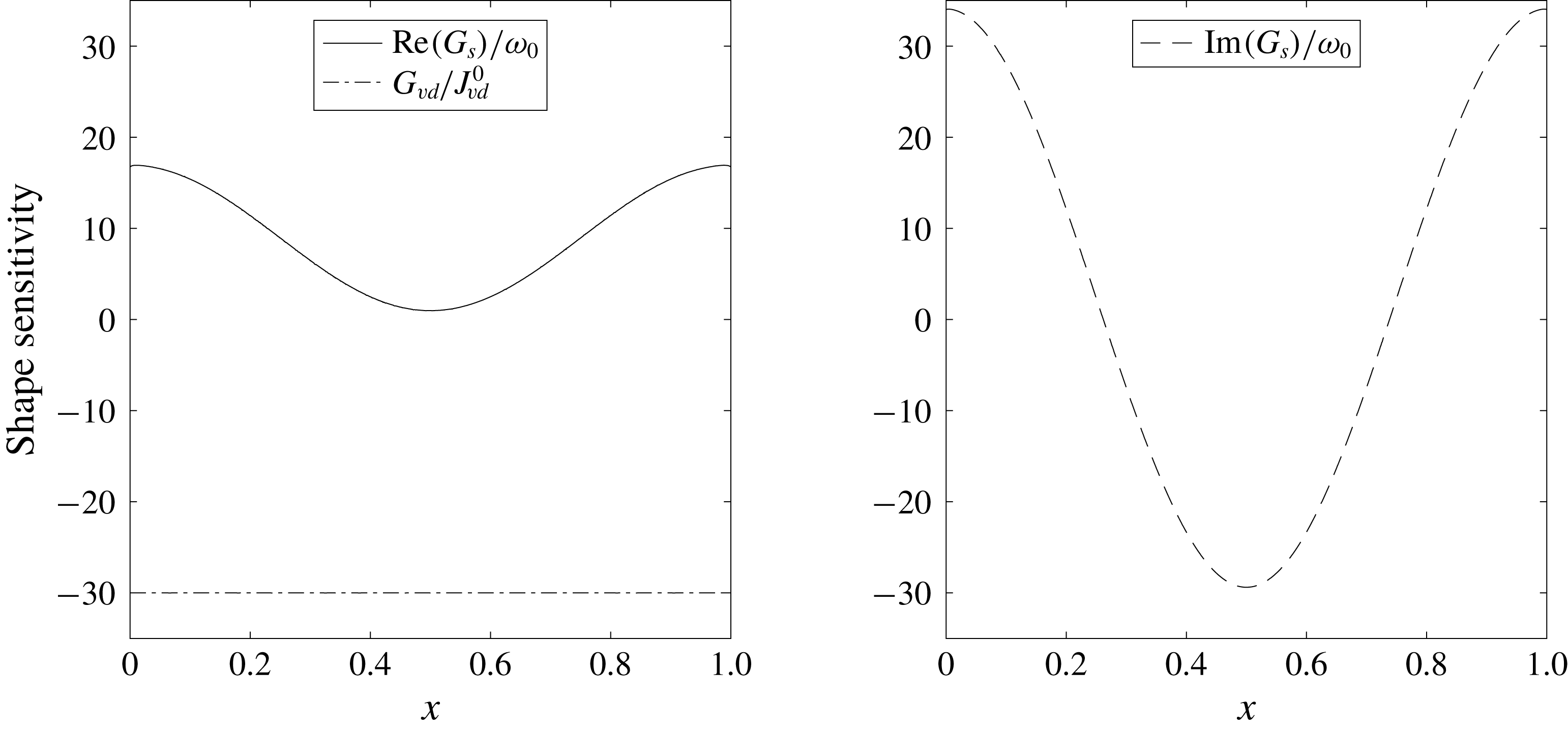
A shape derivative
 $J^{\prime }(\unicode[STIX]{x1D6FA})[V]$
can be written in Hadamard form as a scalar product of a sensitivity functional
$J^{\prime }(\unicode[STIX]{x1D6FA})[V]$
can be written in Hadamard form as a scalar product of a sensitivity functional
 $G(q,q^{+})$
and the normal component of the deformation field
$G(q,q^{+})$
and the normal component of the deformation field
 $V$
, where
$V$
, where
 $q^{+}$
is the adjoint state:
$q^{+}$
is the adjoint state:
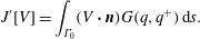 $$\begin{eqnarray}J^{\prime }[V]=\int _{\unicode[STIX]{x1D6E4}_{0}}(V\boldsymbol{\cdot }\boldsymbol{n})G(q,q^{+})\,\text{d}s.\end{eqnarray}$$
In the following sections, we discuss the choice of the objective functions for the steady and the oscillating flows, construct the adjoint states and derive the corresponding sensitivity functionals.
3.2 Steady flow shape sensitivity
For the steady flow, we wish to minimize the viscous dissipation,
 $J_{vd}$
, in the domain:
$J_{vd}$
, in the domain:
 $$\begin{eqnarray}J_{vd}(\bar{u},\unicode[STIX]{x1D6FA})=\int _{\unicode[STIX]{x1D6FA}}\frac{1}{\overline{Re}}(\unicode[STIX]{x1D735}_{j}\bar{u}_{i})^{2}\,\text{d}\boldsymbol{x},\end{eqnarray}$$
where
 $\bar{u}$
satisfies the momentum equation and the divergence-free condition given by (2.13), (2.14). As discussed by Schmidt & Schulz (Reference Schmidt and Schulz2010), the viscous dissipation sensitivity functional
$\bar{u}$
satisfies the momentum equation and the divergence-free condition given by (2.13), (2.14). As discussed by Schmidt & Schulz (Reference Schmidt and Schulz2010), the viscous dissipation sensitivity functional
 $G_{vd}$
for a shape displacement defined on a no-slip surface is
$G_{vd}$
for a shape displacement defined on a no-slip surface is
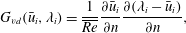 $$\begin{eqnarray}G_{vd}(\bar{u}_{i},\unicode[STIX]{x1D706}_{i})=\frac{1}{\overline{Re}}\frac{\unicode[STIX]{x2202}\bar{u}_{i}}{\unicode[STIX]{x2202}n}\frac{\unicode[STIX]{x2202}(\unicode[STIX]{x1D706}_{i}-\bar{u}_{i})}{\unicode[STIX]{x2202}n},\end{eqnarray}$$
where
 $\unicode[STIX]{x1D706}_{i}$
and
$\unicode[STIX]{x1D706}_{i}$
and
 $\unicode[STIX]{x1D706}_{p}$
are the adjoint velocity and pressure states satisfying
$\unicode[STIX]{x1D706}_{p}$
are the adjoint velocity and pressure states satisfying
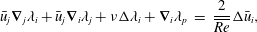 $$\begin{eqnarray}\displaystyle \bar{u}_{j}\unicode[STIX]{x1D735}_{j}\unicode[STIX]{x1D706}_{i}+\bar{u}_{j}\unicode[STIX]{x1D735}_{i}\unicode[STIX]{x1D706}_{j}+\unicode[STIX]{x1D708}\unicode[STIX]{x0394}\unicode[STIX]{x1D706}_{i}+\unicode[STIX]{x1D735}_{i}\unicode[STIX]{x1D706}_{p} & = & \displaystyle \frac{2}{\overline{Re}}\unicode[STIX]{x0394}\bar{u}_{i},\end{eqnarray}$$
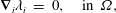 $$\begin{eqnarray}\displaystyle \unicode[STIX]{x1D735}_{i}\unicode[STIX]{x1D706}_{i} & = & \displaystyle 0,\quad \text{in }\unicode[STIX]{x1D6FA},\end{eqnarray}$$
 $$\begin{eqnarray}\displaystyle \unicode[STIX]{x1D706}_{i} & = & \displaystyle 0\quad \text{on }\unicode[STIX]{x1D6E4}_{in}\cup \unicode[STIX]{x1D6E4}_{w},\end{eqnarray}$$
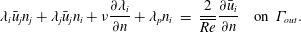 $$\begin{eqnarray}\displaystyle \unicode[STIX]{x1D706}_{i}\bar{u}_{j}n_{j}+\unicode[STIX]{x1D706}_{j}\bar{u}_{j}n_{i}+\unicode[STIX]{x1D708}\frac{\unicode[STIX]{x2202}\unicode[STIX]{x1D706}_{i}}{\unicode[STIX]{x2202}n}+\unicode[STIX]{x1D706}_{p}n_{i} & = & \displaystyle \frac{2}{\overline{Re}}\frac{\unicode[STIX]{x2202}\bar{u}_{i}}{\unicode[STIX]{x2202}n}\quad \text{on }\unicode[STIX]{x1D6E4}_{out}.\end{eqnarray}$$
3.3 Oscillating flow shape sensitivity
For the oscillating flow we wish to control the decay rate and frequency (Luchini & Bottaro Reference Luchini and Bottaro2014), so the objective function is the complex natural frequency,
 $s$
, of the thermoviscous acoustic flow (2.20):
$s$
, of the thermoviscous acoustic flow (2.20):
 $$\begin{eqnarray}J_{s}=s.\end{eqnarray}$$
We introduce an adjoint state vector
 $\boldsymbol{q}^{+}=(P^{+},u_{i}^{+},T^{+})$
containing the adjoint pressure, velocity and temperature variables. Taking the inner product of the direct equations and the corresponding adjoint variables, we construct a Lagrangian of the system (Gunzburger Reference Gunzburger2002),
$\boldsymbol{q}^{+}=(P^{+},u_{i}^{+},T^{+})$
containing the adjoint pressure, velocity and temperature variables. Taking the inner product of the direct equations and the corresponding adjoint variables, we construct a Lagrangian of the system (Gunzburger Reference Gunzburger2002),
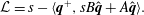 $$\begin{eqnarray}{\mathcal{L}}=s-\langle \boldsymbol{q}^{+},sB\hat{\boldsymbol{q}}+A\hat{\boldsymbol{q}}\rangle .\end{eqnarray}$$
The optimality condition sets any first Lagrangian variation to zero. Variation with respect to the adjoint and direct variables gives the direct and the adjoint state equations, respectively. As discussed in § A.1, the adjoint and the direct states of the thermoviscous acoustic problem are related by
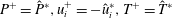 $P^{+}=\hat{P}^{\ast },u_{i}^{+}=-\hat{u} _{i}^{\ast },T^{+}=\hat{T}^{\ast }$
, subject to the normalization condition:
$P^{+}=\hat{P}^{\ast },u_{i}^{+}=-\hat{u} _{i}^{\ast },T^{+}=\hat{T}^{\ast }$
, subject to the normalization condition:
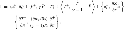 $$\begin{eqnarray}\displaystyle 1 & = & \displaystyle \langle u_{i}^{+},\hat{u} _{i}\rangle +\langle P^{+},\unicode[STIX]{x1D6FE}\hat{P}-\hat{T}\rangle +\left\langle T^{+},\frac{\hat{T}}{\unicode[STIX]{x1D6FE}-1}-\hat{P}\right\rangle +\left\{u_{i}^{+},\frac{\unicode[STIX]{x2202}Z}{\unicode[STIX]{x2202}s}\hat{u} _{i}\right\}\nonumber\\ \displaystyle & & \displaystyle -\left\{\frac{\unicode[STIX]{x2202}T^{+}}{\unicode[STIX]{x2202}n},\frac{(\unicode[STIX]{x2202}\unicode[STIX]{x1D6FC}_{w}/\unicode[STIX]{x2202}s)}{(\unicode[STIX]{x1D6FE}-1)\tilde{Pe}}\frac{\unicode[STIX]{x2202}\hat{T}}{\unicode[STIX]{x2202}n}\right\},\end{eqnarray}$$
where we define the volume inner product
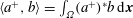 $\langle a^{+},b\rangle =\int _{\unicode[STIX]{x1D6FA}}(a^{+})^{\ast }b\,\text{d}\boldsymbol{x}$
(A 3a
) and the surface inner product
$\langle a^{+},b\rangle =\int _{\unicode[STIX]{x1D6FA}}(a^{+})^{\ast }b\,\text{d}\boldsymbol{x}$
(A 3a
) and the surface inner product
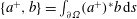 $\{a^{+},b\}=\int _{\unicode[STIX]{x2202}\unicode[STIX]{x1D6FA}}(a^{+})^{\ast }b\,\text{d}s$
(A 3b
).
$\{a^{+},b\}=\int _{\unicode[STIX]{x2202}\unicode[STIX]{x1D6FA}}(a^{+})^{\ast }b\,\text{d}s$
(A 3b
).
For a shape deformation normal to a boundary, the oscillating flow eigenvalue sensitivity
 $G_{s}$
consists of the surface stress and the thermal terms,
$G_{s}$
consists of the surface stress and the thermal terms,
 $G_{s}=G_{s}^{str}+G_{s}^{th}$
(derived in § A.2). Given that the direct and adjoint states are identical up to the sign of the velocity term, the sensitivity functionals are:
$G_{s}=G_{s}^{str}+G_{s}^{th}$
(derived in § A.2). Given that the direct and adjoint states are identical up to the sign of the velocity term, the sensitivity functionals are:
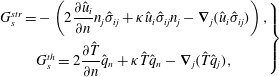 $$\begin{eqnarray}\left.\begin{array}{@{}c@{}}G_{s}^{str}=-\left(2{\displaystyle \frac{\unicode[STIX]{x2202}\hat{u} _{i}}{\unicode[STIX]{x2202}n}}n_{j}\hat{\unicode[STIX]{x1D70E}}_{ij}+\unicode[STIX]{x1D705}\hat{u} _{i}\hat{\unicode[STIX]{x1D70E}}_{ij}n_{j}-\unicode[STIX]{x1D735}_{j}(\hat{u} _{i}\hat{\unicode[STIX]{x1D70E}}_{ij})\right),\\ G_{s}^{th}=2{\displaystyle \frac{\unicode[STIX]{x2202}\hat{T}}{\unicode[STIX]{x2202}n}}\hat{q}_{n}+\unicode[STIX]{x1D705}\hat{T}\hat{q}_{n}-\unicode[STIX]{x1D735}_{j}(\hat{T}\hat{q}_{j}),\end{array}\right\}\end{eqnarray}$$
where
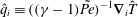 $\hat{q}_{i}\equiv ((\unicode[STIX]{x1D6FE}-1)\tilde{Pe})^{-1}\unicode[STIX]{x1D735}_{i}\hat{T}$
is the boundary heat flux, and
$\hat{q}_{i}\equiv ((\unicode[STIX]{x1D6FE}-1)\tilde{Pe})^{-1}\unicode[STIX]{x1D735}_{i}\hat{T}$
is the boundary heat flux, and
 $\hat{q}_{n}=(\hat{q}\boldsymbol{\cdot }\boldsymbol{n})$
is its normal component. The viscous and the thermal sensitivity functionals have equivalent structure in terms of the
$\hat{q}_{n}=(\hat{q}\boldsymbol{\cdot }\boldsymbol{n})$
is its normal component. The viscous and the thermal sensitivity functionals have equivalent structure in terms of the
 $(\hat{u} _{i},\hat{\unicode[STIX]{x1D70E}}_{ij})$
and
$(\hat{u} _{i},\hat{\unicode[STIX]{x1D70E}}_{ij})$
and
 $(\hat{T},\hat{q}_{i})$
pairs.
$(\hat{T},\hat{q}_{i})$
pairs.
On the no-slip and stress-free boundaries, the viscous sensitivity functional simplifies to
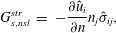 $$\begin{eqnarray}\displaystyle G_{s,nsl}^{str} & = & \displaystyle -\frac{\unicode[STIX]{x2202}\hat{u} _{i}}{\unicode[STIX]{x2202}n}n_{j}\hat{\unicode[STIX]{x1D70E}}_{ij},\end{eqnarray}$$
 $$\begin{eqnarray}\displaystyle G_{s,free}^{str} & = & \displaystyle \unicode[STIX]{x1D735}_{j}(\hat{u} _{i}\hat{\unicode[STIX]{x1D70E}}_{ij}),\end{eqnarray}$$
 $$\begin{eqnarray}\displaystyle G_{s,iso}^{th} & = & \displaystyle \frac{\unicode[STIX]{x2202}\hat{T}}{\unicode[STIX]{x2202}n}\hat{q}_{n},\end{eqnarray}$$
 $$\begin{eqnarray}\displaystyle G_{s,ad}^{th} & = & \displaystyle -\unicode[STIX]{x1D735}_{j}(\hat{T}\hat{q}_{j}).\end{eqnarray}$$
4 Shape optimization in a 2-D channel
4.1 Numerical methods
4.1.1 Optimization domain
We start with a flow in a two-dimensional uniform-width channel, defined as
 $$\begin{eqnarray}\unicode[STIX]{x1D6FA}_{0}=\{(x,y)\in \mathbb{R}^{2}\mid [0,1]\times [0,0.1]\},\end{eqnarray}$$
with inlet and outlet boundaries
 $$\begin{eqnarray}\displaystyle \unicode[STIX]{x1D6E4}_{in,0} & = & \displaystyle \{(x,y)\in \mathbb{R}^{2}\mid x=0\},\end{eqnarray}$$
 $$\begin{eqnarray}\displaystyle \unicode[STIX]{x1D6E4}_{out,0} & = & \displaystyle \{(x,y)\in \mathbb{R}^{2}\mid x=1\},\end{eqnarray}$$
 $\unicode[STIX]{x1D6E4}_{w,0}=\unicode[STIX]{x2202}\unicode[STIX]{x1D6FA}_{0}\backslash (\unicode[STIX]{x1D6E4}_{in,0}\cup \unicode[STIX]{x1D6E4}_{out,0})$
. For the oscillating flow, the stress-free boundary is
$\unicode[STIX]{x1D6E4}_{w,0}=\unicode[STIX]{x2202}\unicode[STIX]{x1D6FA}_{0}\backslash (\unicode[STIX]{x1D6E4}_{in,0}\cup \unicode[STIX]{x1D6E4}_{out,0})$
. For the oscillating flow, the stress-free boundary is
 $\unicode[STIX]{x1D6E4}_{free,0}=\unicode[STIX]{x1D6E4}_{in,0}\cup \unicode[STIX]{x1D6E4}_{out,0}$
.
$\unicode[STIX]{x1D6E4}_{free,0}=\unicode[STIX]{x1D6E4}_{in,0}\cup \unicode[STIX]{x1D6E4}_{out,0}$
. The boundary
 $\unicode[STIX]{x1D6E4}_{w,0}$
is to be optimized by modifying the no-slip boundaries, while fixing the inlet and the outlet. If equivalent boundary displacement fields are applied to the top and the bottom no-slip surfaces then the steady flow and the oscillating flow boundary sensitivities and the shape gradients remain symmetric. Therefore we may consider deformation of only the top boundary.
$\unicode[STIX]{x1D6E4}_{w,0}$
is to be optimized by modifying the no-slip boundaries, while fixing the inlet and the outlet. If equivalent boundary displacement fields are applied to the top and the bottom no-slip surfaces then the steady flow and the oscillating flow boundary sensitivities and the shape gradients remain symmetric. Therefore we may consider deformation of only the top boundary.
In this study, we parametrize the boundary with a set of
 $N$
control points
$N$
control points
 $\{a^{k}\in \mathbb{R}^{2}\mid k=1\ldots N\}$
defining the third-order rational uniform B-spline curve. This provides a smooth surface of class
$\{a^{k}\in \mathbb{R}^{2}\mid k=1\ldots N\}$
defining the third-order rational uniform B-spline curve. This provides a smooth surface of class
 $C^{2}$
for which parametric sensitivities can be calculated (Samareh Reference Samareh2001). Boundary displacement fields,
$C^{2}$
for which parametric sensitivities can be calculated (Samareh Reference Samareh2001). Boundary displacement fields,
 $V^{k}$
, are, by definition, the boundary shape sensitivities to the control point positions,
$V^{k}$
, are, by definition, the boundary shape sensitivities to the control point positions,
 $$\begin{eqnarray}V^{k}=\frac{\unicode[STIX]{x2202}\unicode[STIX]{x1D6E4}_{w}}{\unicode[STIX]{x2202}a^{k}},\end{eqnarray}$$
which implies that the objective function gradient with respect to the displacement field
 $J^{\prime }[V^{k}]$
transforms to the sensitivity with respect to the control parameters,
$J^{\prime }[V^{k}]$
transforms to the sensitivity with respect to the control parameters,
 $J^{\prime }[a^{k}]$
. As the positions of the control points are moved in the gradient direction, the domain is updated and the computational mesh is rebuilt.
$J^{\prime }[a^{k}]$
. As the positions of the control points are moved in the gradient direction, the domain is updated and the computational mesh is rebuilt.
We parametrize the top boundary of the initial rectangular domain with 11 control points,
 $a_{i}=(i/10,0.1)$
,
$a_{i}=(i/10,0.1)$
,
 $i=0\ldots 10$
, spaced uniformly at intervals of
$i=0\ldots 10$
, spaced uniformly at intervals of
 $0.1$
. The first and last points are kept at their initial positions so that the inlet and outlet boundaries are fixed and the channel’s length remains equal to 1.
$0.1$
. The first and last points are kept at their initial positions so that the inlet and outlet boundaries are fixed and the channel’s length remains equal to 1.
4.1.2 Numerical discretization
We use a finite element method for spatial discretization. The direct and adjoint formulations of the steady flow problem and the direct formulation of the oscillating flow problem are first written in a variational form and then discretized using the Fenics finite elements solver (Logg, Mardal & Wells Reference Logg, Mardal and Wells2012) on a mesh of triangular elements generated by Gmsh (Geuzaine & Remacle Reference Geuzaine and Remacle2009). The velocity and pressure fields
 $(\bar{u}_{i},\bar{P})$
(2.13), (2.14) and the adjoint fields
$(\bar{u}_{i},\bar{P})$
(2.13), (2.14) and the adjoint fields
 $(\unicode[STIX]{x1D706}_{i},\unicode[STIX]{x1D706}_{p})$
(3.9) for the steady flow are discretized using Taylor–Hood
$(\unicode[STIX]{x1D706}_{i},\unicode[STIX]{x1D706}_{p})$
(3.9) for the steady flow are discretized using Taylor–Hood
 $(\text{P}_{2},\text{P}_{1})$
elements. The acoustic perturbation field
$(\text{P}_{2},\text{P}_{1})$
elements. The acoustic perturbation field
 $(\tilde{P},\tilde{u} _{i},\tilde{T})$
(2.20) is discretized using
$(\tilde{P},\tilde{u} _{i},\tilde{T})$
(2.20) is discretized using
 $\left(\text{P}_{1},\text{P}_{2},\text{P}_{2}\right)$
elements (see Kampinga, Wijnant & de Boer Reference Kampinga, Wijnant and de Boer2010). The resulting discrete sparse matrices are inverted by a direct lower–upper (LU) solver using a multifrontal massively parallel sparse direct solver (MUMPS).
$\left(\text{P}_{1},\text{P}_{2},\text{P}_{2}\right)$
elements (see Kampinga, Wijnant & de Boer Reference Kampinga, Wijnant and de Boer2010). The resulting discrete sparse matrices are inverted by a direct lower–upper (LU) solver using a multifrontal massively parallel sparse direct solver (MUMPS).
For the steady flow problem, the Dirichlet-type boundary conditions are set up strongly for each boundary degree of freedom and the outlet boundary condition is enforced weakly. The nonlinear direct flow is solved using a Newton iterative method. The steady flow inlet velocity profile is parabolic. The oscillating flow problem is a generalized eigenvalue problem and is solved with a shift-invert method from an initial guess.
The oscillating flow viscous and thermal boundary layers are resolved using triangular elements. We apply the goal-oriented adjoint-based error control technique (Rognes & Logg Reference Rognes and Logg2013) for the automated adaptive mesh refinement. The goal functional in our case is the target eigenvalue.
4.1.3 Constrained gradient optimization
Our goals are to decrease the steady flow viscous dissipation and make the oscillation’s decay rate,
 $-\unicode[STIX]{x1D70E}$
, more negative. There is a trade-off between these goals, so here we set the steady flow dissipation as an inequality constraint and minimize
$-\unicode[STIX]{x1D70E}$
, more negative. There is a trade-off between these goals, so here we set the steady flow dissipation as an inequality constraint and minimize
 $\text{Re}(s)$
.
$\text{Re}(s)$
.
 $$\begin{eqnarray}\displaystyle \min _{\unicode[STIX]{x1D6FA}} & & \displaystyle \quad \text{Re}(s)\end{eqnarray}$$
 $$\begin{eqnarray}\displaystyle \text{subject to} & & \displaystyle \quad J_{vd}\leqslant J_{vd}^{0}\end{eqnarray}$$
 $$\begin{eqnarray}\displaystyle \text{and} & & \displaystyle \quad \text{state equations }(2.13),(2.20).\end{eqnarray}$$
In § A.1 we derive shape gradients in Hadamard form of both the objective function and the constraint with respect to an arbitrary boundary displacement
 $V$
. The parameter-based approach restricts the number of possible boundary deformations to the number of control parameters. Essentially, a parametrization projects the function space of the admissible shape deformations onto a lower-dimensional subspace, which allows us to operate with the vector representation of shape gradients instead of the continuous boundary sensitivities.
$V$
. The parameter-based approach restricts the number of possible boundary deformations to the number of control parameters. Essentially, a parametrization projects the function space of the admissible shape deformations onto a lower-dimensional subspace, which allows us to operate with the vector representation of shape gradients instead of the continuous boundary sensitivities.
We can estimate the optimality of a shape (but not the parametrization) by considering the scalar product of the objective shape sensitivity,
 $G$
, with the constraint shape sensitivity,
$G$
, with the constraint shape sensitivity,
 $G^{\prime }$
. The surface inner product
$G^{\prime }$
. The surface inner product
 $\{G,G^{\prime }\}$
(A 3) and the surface norm
$\{G,G^{\prime }\}$
(A 3) and the surface norm
 $\Vert G\Vert _{\unicode[STIX]{x1D6E4}}^{2}=\{G,G\}$
form the optimality coefficient
$\Vert G\Vert _{\unicode[STIX]{x1D6E4}}^{2}=\{G,G\}$
form the optimality coefficient
 $\unicode[STIX]{x1D6FC}$
:
$\unicode[STIX]{x1D6FC}$
:
 $$\begin{eqnarray}\unicode[STIX]{x1D6FC}=\frac{\{G,G^{\prime }\}}{\Vert G\Vert _{\unicode[STIX]{x1D6E4}}\Vert G^{\prime }\Vert _{\unicode[STIX]{x1D6E4}}}\geqslant -1.\end{eqnarray}$$
The optimality coefficient indicates the cosine of the angle between the objective function shape sensitivity and the constraint shape sensitivity, such that
 $\unicode[STIX]{x1D6FC}=-1$
implies that they point in opposite directions and the system has reached its local optimum. In the case of
$\unicode[STIX]{x1D6FC}=-1$
implies that they point in opposite directions and the system has reached its local optimum. In the case of
 $N$
optimization parameters, a sensitivity functional is realized on a shape deformation subspace, spanned by
$N$
optimization parameters, a sensitivity functional is realized on a shape deformation subspace, spanned by
 $V^{k}$
,
$V^{k}$
,
 $k=1\ldots N$
. The discrete gradient vector
$k=1\ldots N$
. The discrete gradient vector
 $\boldsymbol{g}\in \mathbb{R}^{N}$
is defined as
$\boldsymbol{g}\in \mathbb{R}^{N}$
is defined as
 $\boldsymbol{g}_{k}=\{V^{k},G\}$
, and the parametric optimality coefficient
$\boldsymbol{g}_{k}=\{V^{k},G\}$
, and the parametric optimality coefficient
 $\unicode[STIX]{x1D6FC}_{p}$
is:
$\unicode[STIX]{x1D6FC}_{p}$
is:
 $$\begin{eqnarray}\unicode[STIX]{x1D6FC}_{p}=\frac{\boldsymbol{g}^{\text{T}}\boldsymbol{g}^{\prime }}{\Vert \boldsymbol{g}\Vert \boldsymbol{\cdot }\Vert \boldsymbol{g}^{\prime }\Vert }\leqslant \unicode[STIX]{x1D6FC}.\end{eqnarray}$$
In the parameter-based optimization,
 $\unicode[STIX]{x1D6FC}_{p}=-1$
implies that the local optimum has been reached within the choice of parametrization.
$\unicode[STIX]{x1D6FC}_{p}=-1$
implies that the local optimum has been reached within the choice of parametrization.
The optimization algorithm for the problem (4.4) is based on the method of moving asymptotes (Svanberg Reference Svanberg1987). The objective and the constraint values and their gradients are calculated by (i) solving the steady flow (2.13) and the oscillating eigenvalue (2.20) problems, (ii) finding the adjoint steady flow (3.9) and oscillating flow (3.12) states, (iii) calculating the boundary sensitivities
 $G_{vd},G_{s}$
using (3.8) and (3.13), and computing the objective and constraint gradients with respect to the boundary control points
$G_{vd},G_{s}$
using (3.8) and (3.13), and computing the objective and constraint gradients with respect to the boundary control points
 $s^{\prime }[a_{k}]=\{V^{k},G_{s}\},J_{vd}^{\prime }[a_{k}]=\{V^{k},G_{vd}\}$
. We use
$s^{\prime }[a_{k}]=\{V^{k},G_{s}\},J_{vd}^{\prime }[a_{k}]=\{V^{k},G_{vd}\}$
. We use
 $\unicode[STIX]{x1D700}_{p}=\unicode[STIX]{x1D6FC}_{p}+1$
as a tolerance criteria for the optimization process.
$\unicode[STIX]{x1D700}_{p}=\unicode[STIX]{x1D6FC}_{p}+1$
as a tolerance criteria for the optimization process.
4.2 Optimization results
4.2.1 Initial domain
The steady flow is computed in the initially flat channel (4.1) at
 $\overline{Re}=0.1$
with a parabolic inflow velocity profile. In the unaltered domain this results in the Poiseuille flow solution, and the corresponding viscous dissipation value
$\overline{Re}=0.1$
with a parabolic inflow velocity profile. In the unaltered domain this results in the Poiseuille flow solution, and the corresponding viscous dissipation value
 $J_{vd}^{0}$
is taken as a reference. For the oscillating flow at
$J_{vd}^{0}$
is taken as a reference. For the oscillating flow at
 $\tilde{Re}=1000$
, we choose the smallest non-zero-frequency natural mode as the target mode, with
$\tilde{Re}=1000$
, we choose the smallest non-zero-frequency natural mode as the target mode, with
 $s_{0}=-0.555+2.81\text{i}$
. Figure 1 shows the real and imaginary parts of the mode shape, normalized by (3.12). The pressure gradient
$s_{0}=-0.555+2.81\text{i}$
. Figure 1 shows the real and imaginary parts of the mode shape, normalized by (3.12). The pressure gradient
 $\unicode[STIX]{x2202}_{x}\hat{P}$
and the longitudinal velocity
$\unicode[STIX]{x2202}_{x}\hat{P}$
and the longitudinal velocity
 $\hat{u} _{x}$
are highest on the stress-free open end boundaries at
$\hat{u} _{x}$
are highest on the stress-free open end boundaries at
 $x=0,x=1$
. As indicated in figure 2, the regions with the highest contribution to the decay rate
$x=0,x=1$
. As indicated in figure 2, the regions with the highest contribution to the decay rate
 $\unicode[STIX]{x1D70E}_{\unicode[STIX]{x1D6FA}}$
are the no-slip wall regions close to the open ends, where the velocity magnitude isolines converge and therefore the transverse velocity gradient is the largest. For the initial channel configuration,
$\unicode[STIX]{x1D70E}_{\unicode[STIX]{x1D6FA}}$
are the no-slip wall regions close to the open ends, where the velocity magnitude isolines converge and therefore the transverse velocity gradient is the largest. For the initial channel configuration,
 $\unicode[STIX]{x1D6FC}_{p}=-0.7$
.
$\unicode[STIX]{x1D6FC}_{p}=-0.7$
.

Figure 1. First natural mode of the oscillating flow in a flat channel at
 $\tilde{Re}=1000$
. (a–h) Pressure
$\tilde{Re}=1000$
. (a–h) Pressure
 $\hat{P}$
, longitudinal
$\hat{P}$
, longitudinal
 $\hat{u} _{x}$
and transverse
$\hat{u} _{x}$
and transverse
 $\hat{u} _{y}$
velocity components, and temperature
$\hat{u} _{y}$
velocity components, and temperature
 $\hat{T}$
mode shapes; real (a,c,e,g) and imaginary (b,d,f,h) parts.
$\hat{T}$
mode shapes; real (a,c,e,g) and imaginary (b,d,f,h) parts.

Figure 2. Spatial distribution of the decay rate production
 $\unicode[STIX]{x1D70E}_{\unicode[STIX]{x1D6FA}}$
in a flat channel. Black lines correspond to the oscillating flow velocity magnitude isolines
$\unicode[STIX]{x1D70E}_{\unicode[STIX]{x1D6FA}}$
in a flat channel. Black lines correspond to the oscillating flow velocity magnitude isolines
 $\hat{u} =\text{const}.$
The steady flow state in the unperturbed channel is independent of the longitudinal coordinate
 $x$
so the viscous dissipation shape sensitivity
$x$
so the viscous dissipation shape sensitivity
 $G_{vd}(\bar{u}_{i},\unicode[STIX]{x1D706}_{i})$
is constant along the no-slip walls (figure 3). Here, and later,
$G_{vd}(\bar{u}_{i},\unicode[STIX]{x1D706}_{i})$
is constant along the no-slip walls (figure 3). Here, and later,
 $G_{vd}$
is normalized by the viscous dissipation value
$G_{vd}$
is normalized by the viscous dissipation value
 $J_{vd}^{0}$
in the starting geometry configuration. The shape sensitivity
$J_{vd}^{0}$
in the starting geometry configuration. The shape sensitivity
 $G_{vd}$
is always negative, so any boundary displacement resulting in contraction of the channel’s width leads to growth of viscous dissipation. The complex eigenvalue shape sensitivity
$G_{vd}$
is always negative, so any boundary displacement resulting in contraction of the channel’s width leads to growth of viscous dissipation. The complex eigenvalue shape sensitivity
 $G_{s}(\hat{P},\hat{u} _{i},\hat{T})$
is not uniform; the real part
$G_{s}(\hat{P},\hat{u} _{i},\hat{T})$
is not uniform; the real part
 $\text{Re}(G_{s})$
is almost zero in the middle part of the boundary and grows towards the channel’s open ends where the decay rate production is highest, as shown previously. As for viscous dissipation, any shape deformation directed inwards
$\text{Re}(G_{s})$
is almost zero in the middle part of the boundary and grows towards the channel’s open ends where the decay rate production is highest, as shown previously. As for viscous dissipation, any shape deformation directed inwards
 $(V\boldsymbol{\cdot }\boldsymbol{n})<0$
leads to an increase in the decay rate magnitude.
$(V\boldsymbol{\cdot }\boldsymbol{n})<0$
leads to an increase in the decay rate magnitude.

Figure 3. Shape sensitivity distribution along the flat channel top boundary for the decay rate
 $\text{Re}(G_{s})$
(solid line) and frequency
$\text{Re}(G_{s})$
(solid line) and frequency
 $\text{Im}(G_{s})$
(dashed line) of the first oscillating mode, and the steady flow viscous dissipation shape sensitivity
$\text{Im}(G_{s})$
(dashed line) of the first oscillating mode, and the steady flow viscous dissipation shape sensitivity
 $G_{vd}/J_{0}$
normalized by viscous dissipation inside the channel (dotted line).
$G_{vd}/J_{0}$
normalized by viscous dissipation inside the channel (dotted line).
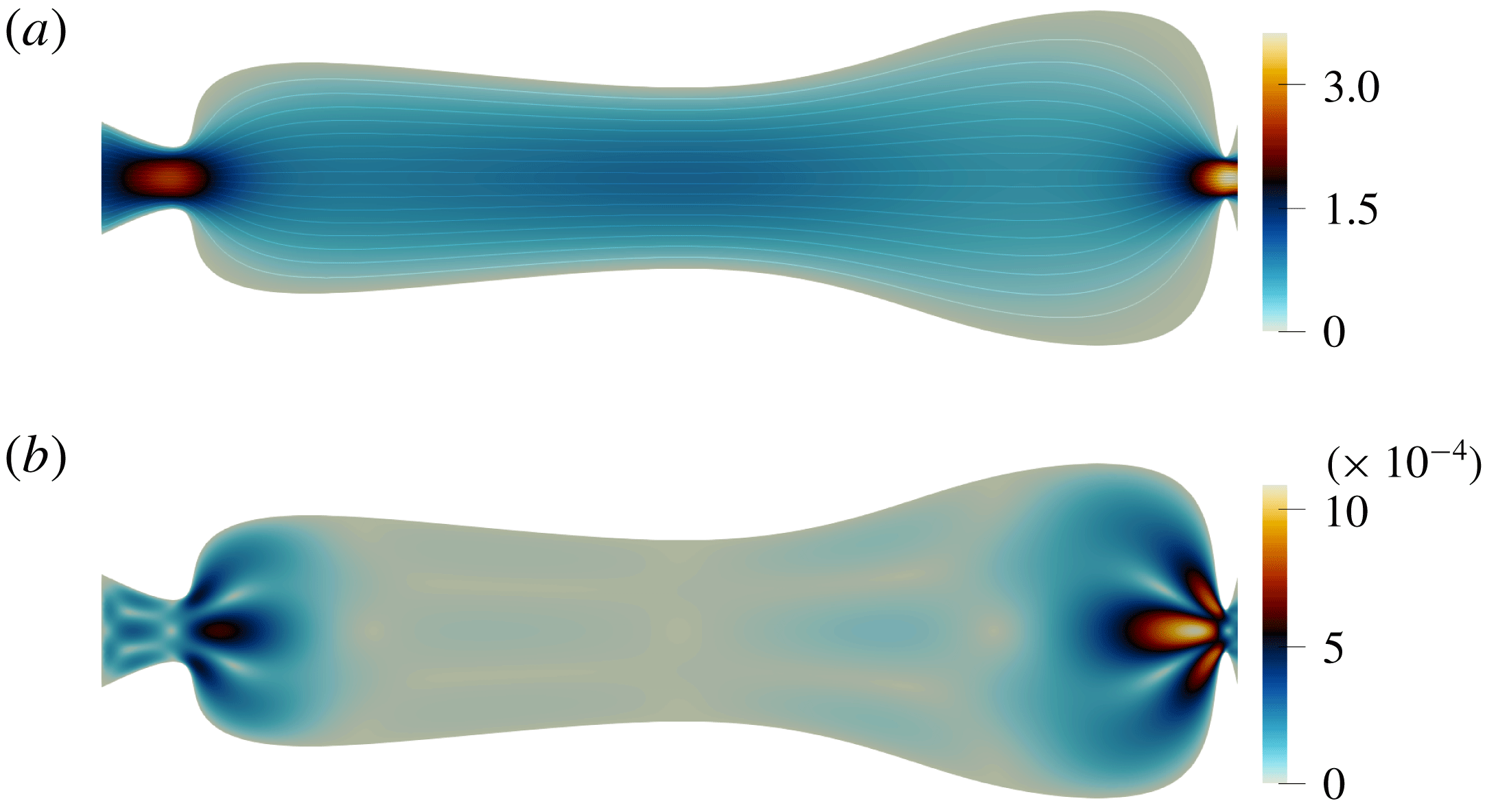
Figure 4. Steady flow in the optimized channel at
 $\overline{Re}=0.1$
. (a) The direct steady flow
$\overline{Re}=0.1$
. (a) The direct steady flow
 $|\bar{u}|$
velocity magnitude, with the streamlines indicated (solid lines). (b) The adjoint steady flow
$|\bar{u}|$
velocity magnitude, with the streamlines indicated (solid lines). (b) The adjoint steady flow
 $|\unicode[STIX]{x1D706}|$
velocity magnitude.
$|\unicode[STIX]{x1D706}|$
velocity magnitude.
As indicated in figure 3, the decay rate is less sensitive to shape modifications in the middle region of the channel at
 $0.3\leqslant x\leqslant 0.7$
, and has higher sensitivity on the outer region. We expect therefore, that the channel will expand in the middle and shrink around the free boundaries to increase the decay rate while keeping the steady flow viscous dissipation constant. This is also what we expect on physical grounds: the channels will constrict where the acoustic velocity is greater.
$0.3\leqslant x\leqslant 0.7$
, and has higher sensitivity on the outer region. We expect therefore, that the channel will expand in the middle and shrink around the free boundaries to increase the decay rate while keeping the steady flow viscous dissipation constant. This is also what we expect on physical grounds: the channels will constrict where the acoustic velocity is greater.
4.2.2 Optimized domain
The optimized configuration is found in 20 iterations and has the optimality coefficient (4.5) of
 $\unicode[STIX]{x1D6FC}_{p}=-0.98$
. The first eigenmode in the optimized channel is
$\unicode[STIX]{x1D6FC}_{p}=-0.98$
. The first eigenmode in the optimized channel is
 $s=-1.31+1.68i$
. In comparison to the initial solution, the decay rate objective function changes by almost 140 %, and the frequency (which is unconstrained) decreases by 40 %. The total area almost doubles and the channel’s shape loses symmetry around the
$s=-1.31+1.68i$
. In comparison to the initial solution, the decay rate objective function changes by almost 140 %, and the frequency (which is unconstrained) decreases by 40 %. The total area almost doubles and the channel’s shape loses symmetry around the
 $x=0.5$
vertical plane, while remaining symmetric in the horizontal plane. The channel constricts near
$x=0.5$
vertical plane, while remaining symmetric in the horizontal plane. The channel constricts near
 $x=0.07$
and
$x=0.07$
and
 $x=0.99$
, and the middle part of the channel expands, as expected.
$x=0.99$
, and the middle part of the channel expands, as expected.
Figure 4 shows the steady flow (a) and the adjoint flow (b) velocity magnitude
 $\bar{u}$
and
$\bar{u}$
and
 $\unicode[STIX]{x1D706}$
for the optimized channel. The lines correspond to the steady flow streamlines. The no-slip boundaries are smooth and the flow remains attached to the walls with no recirculation zones. Viscous dissipation in the optimized channel is the same as in the initial channel.
$\unicode[STIX]{x1D706}$
for the optimized channel. The lines correspond to the steady flow streamlines. The no-slip boundaries are smooth and the flow remains attached to the walls with no recirculation zones. Viscous dissipation in the optimized channel is the same as in the initial channel.
The steady flow velocity amplitude and velocity gradients as well as the adjoint velocity are highest in the constricted areas. This makes the constricted regions much more sensitive to shape changes than the expanded part, where the adjoint velocity magnitude is almost zero.
The decay rate production is initially located in the corner regions of the uniform-width channel. When the boundaries shift, this region shifts inside the channel towards the constrictions, as indicated in figure 5. The decay rate production strongly concentrates in the narrow parts of the channel, with the maximum at
 $x=0.99$
more than 10 000 times higher than the average value. It is almost zero between the constrictions.
$x=0.99$
more than 10 000 times higher than the average value. It is almost zero between the constrictions.

Figure 5. Spatial distribution of the absolute value of the decay rate production in the optimized channel (on a logarithmic scale),
 $\ln (-\unicode[STIX]{x1D70E}_{\unicode[STIX]{x1D6FA}})$
. Black lines correspond to the oscillating flow velocity magnitude isolines
$\ln (-\unicode[STIX]{x1D70E}_{\unicode[STIX]{x1D6FA}})$
. Black lines correspond to the oscillating flow velocity magnitude isolines
 $\hat{u} =\text{const.}$
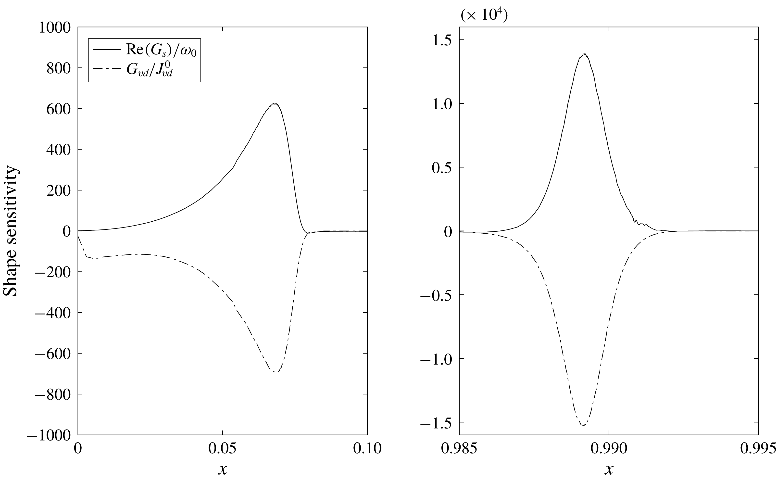
Figure 6. The decay rate shape sensitivity distribution (solid line) of the first oscillating mode in the optimized channel, and the steady flow viscous dissipation sensitivity (dotted line) normalized by viscous dissipation inside the channel.
Figure 6 illustrates the viscous dissipation
 $G_{vd}/J_{vd}^{0}$
(dash-dotted line) and the decay rate
$G_{vd}/J_{vd}^{0}$
(dash-dotted line) and the decay rate
 $\text{Re}(G_{s})/\unicode[STIX]{x1D714}_{0}$
(solid line) boundary sensitivities as functions of the longitudinal coordinate along the top boundary in the optimized channel. Both sensitivities reach their extreme values in the constricted areas and are much smaller in the intermediate region. They are almost equal and opposite to each other, showing that the design is almost optimal. Further improvements can still be made, for instance, by boundary re-parametrization or by introducing additional control points. However, this simple problem has achieved its purpose by showing that the optimization procedure can indeed increase acoustic dissipation while keeping the steady flow dissipation constant.
$\text{Re}(G_{s})/\unicode[STIX]{x1D714}_{0}$
(solid line) boundary sensitivities as functions of the longitudinal coordinate along the top boundary in the optimized channel. Both sensitivities reach their extreme values in the constricted areas and are much smaller in the intermediate region. They are almost equal and opposite to each other, showing that the design is almost optimal. Further improvements can still be made, for instance, by boundary re-parametrization or by introducing additional control points. However, this simple problem has achieved its purpose by showing that the optimization procedure can indeed increase acoustic dissipation while keeping the steady flow dissipation constant.
5 Shape optimization for a 2-D generic inkjet printhead
5.1 Generic geometry and shape parametrization

Figure 7. A 2-D generic printhead geometry with a piezo-electric actuator. The channel is connected to the ink supply manifolds via the inlet and outlet boundaries. Circles denote the B-spline boundary control points. All sizes are in
 $\unicode[STIX]{x03BC}\text{m}$
.
$\unicode[STIX]{x03BC}\text{m}$
.
Figure 7 shows a 2-D generic inkjet printhead chamber, which consists of a vertical inlet and outlet, connected to ink manifolds, and a horizontal main channel. The manifold cross-sections are much larger than the printhead cross-section. A
 $30~\unicode[STIX]{x03BC}\text{m}$
long conical printing nozzle, which has a
$30~\unicode[STIX]{x03BC}\text{m}$
long conical printing nozzle, which has a
 $20~\unicode[STIX]{x03BC}\text{m}$
outer diameter and a taper of
$20~\unicode[STIX]{x03BC}\text{m}$
outer diameter and a taper of
 $8^{\circ }$
, is located in the middle of the printhead. A flat piezo-electric membrane is located on the top boundary opposite the nozzle. In three dimensions, the channel has a depth of
$8^{\circ }$
, is located in the middle of the printhead. A flat piezo-electric membrane is located on the top boundary opposite the nozzle. In three dimensions, the channel has a depth of
 $60~\unicode[STIX]{x03BC}\text{m}$
into the page. For this study, we approximate the channel to be uniform in that direction and examine only 2-D deformations, as in § 4.2. We aim to increase the decay rate of the oscillating flow while keeping the steady flow viscous dissipation constant.
$60~\unicode[STIX]{x03BC}\text{m}$
into the page. For this study, we approximate the channel to be uniform in that direction and examine only 2-D deformations, as in § 4.2. We aim to increase the decay rate of the oscillating flow while keeping the steady flow viscous dissipation constant.
We parametrize the printhead walls by third-order B-splines with the control points indicated in figure 7. The inlet and the outlet points are fixed. The nozzle shape cannot change but it can move in the vertical direction. The bottom wall cannot extend below the nozzle tip.
We choose a characteristic length
 $L=100~\unicode[STIX]{x03BC}\text{m}$
. The steady flow Reynolds number is
$L=100~\unicode[STIX]{x03BC}\text{m}$
. The steady flow Reynolds number is
 $\overline{Re}=0.066$
and the Reynolds number based on the speed of sound is
$\overline{Re}=0.066$
and the Reynolds number based on the speed of sound is
 $\tilde{Re}=6000$
. The steady flow Mach number is
$\tilde{Re}=6000$
. The steady flow Mach number is
 $\unicode[STIX]{x1D707}=10^{-4}$
and the oscillating flow Mach number is
$\unicode[STIX]{x1D707}=10^{-4}$
and the oscillating flow Mach number is
 $\unicode[STIX]{x1D716}=10^{-5}$
. For the steady flow, the inlet has a fixed parabolic velocity profile, the outlet is an open end with stress-free boundary condition (2.14c
) and the walls are no-slip boundaries and the nozzle exit is modelled as a no-slip boundary because there is no flow through it. For the acoustic flow, the walls are adiabatic no slip, and the open boundaries, including the nozzle exit, are stress free and isothermal. In this study we neglect the surface tension at the nozzle exit.
$\unicode[STIX]{x1D716}=10^{-5}$
. For the steady flow, the inlet has a fixed parabolic velocity profile, the outlet is an open end with stress-free boundary condition (2.14c
) and the walls are no-slip boundaries and the nozzle exit is modelled as a no-slip boundary because there is no flow through it. For the acoustic flow, the walls are adiabatic no slip, and the open boundaries, including the nozzle exit, are stress free and isothermal. In this study we neglect the surface tension at the nozzle exit.
Figure 8 shows the steady flow direct
 $\bar{u}$
and adjoint
$\bar{u}$
and adjoint
 $\unicode[STIX]{x1D706}$
velocity magnitude in the initial geometry. The largest direct velocity magnitude is in the narrow horizontal channel. The adjoint velocity has highest value near the sharp corners at the channel entrance and the nozzle. These regions have the greatest influence on the steady flow viscous dissipation.
$\unicode[STIX]{x1D706}$
velocity magnitude in the initial geometry. The largest direct velocity magnitude is in the narrow horizontal channel. The adjoint velocity has highest value near the sharp corners at the channel entrance and the nozzle. These regions have the greatest influence on the steady flow viscous dissipation.
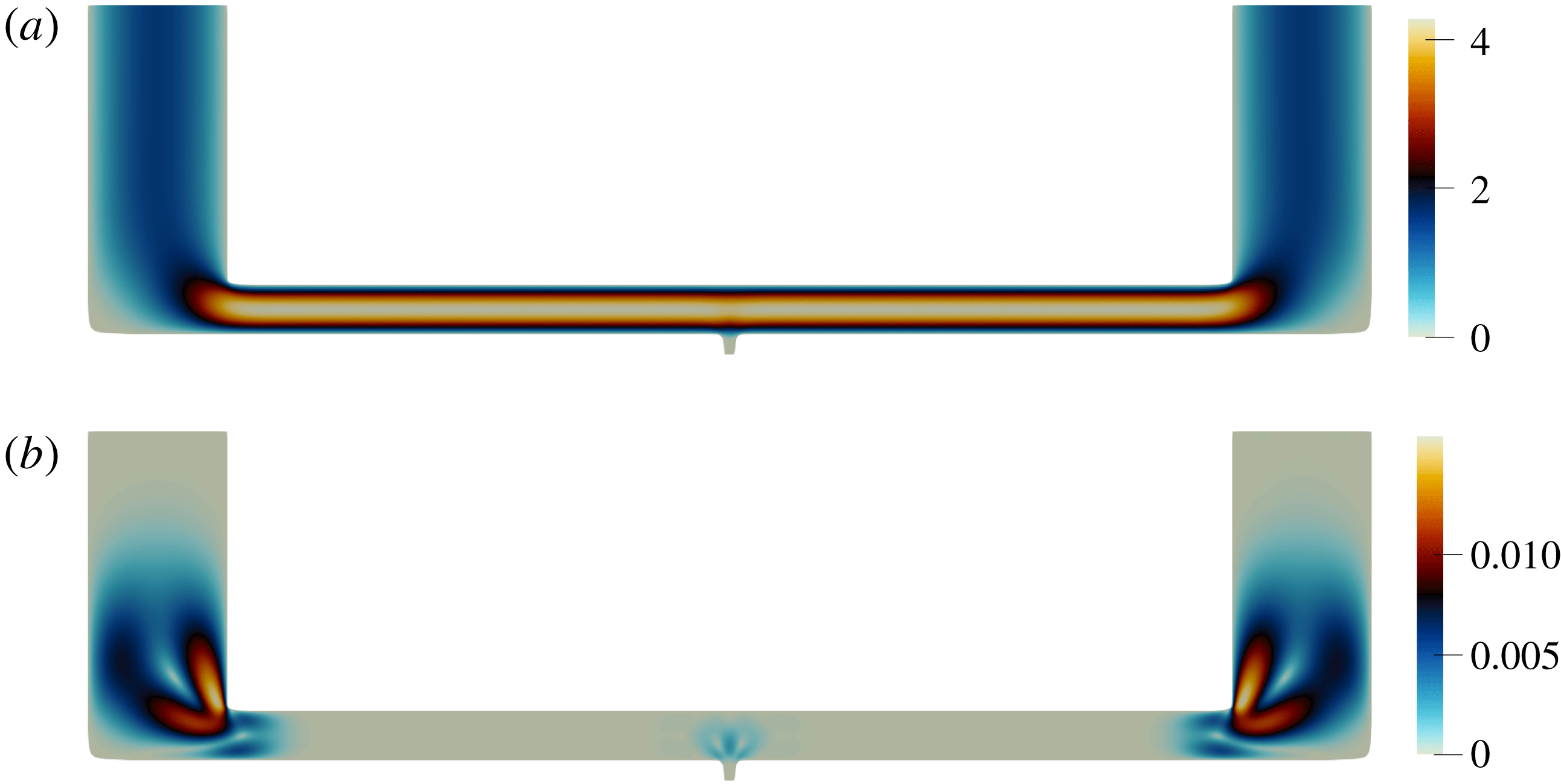
Figure 8. The direct velocity magnitude
 $\bar{u}$
(a) and the adjoint velocity magnitude
$\bar{u}$
(a) and the adjoint velocity magnitude
 $\unicode[STIX]{x1D706}$
(b) of the steady flow in the initial printhead channel at
$\unicode[STIX]{x1D706}$
(b) of the steady flow in the initial printhead channel at
 $\overline{Re}=0.066$
.
$\overline{Re}=0.066$
.
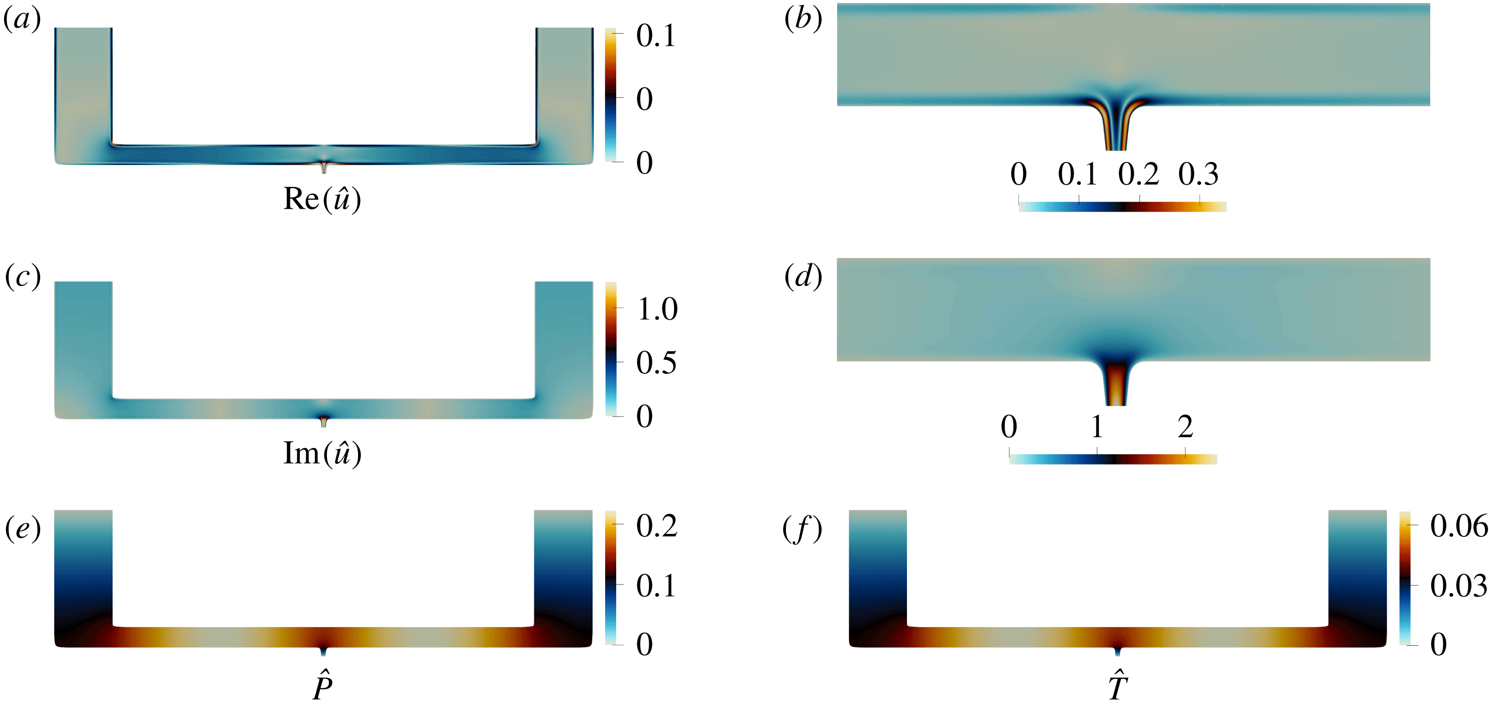
Figure 9. The first natural mode of the oscillating flow in the initial printhead geometry at
 $\tilde{Re}=6000$
. (a,b) The magnitude of the velocity mode real part
$\tilde{Re}=6000$
. (a,b) The magnitude of the velocity mode real part
 $\text{Re}(\hat{u} )$
in the entire domain (a) and near the nozzle (b); (c,d) the magnitude of the velocity mode imaginary part
$\text{Re}(\hat{u} )$
in the entire domain (a) and near the nozzle (b); (c,d) the magnitude of the velocity mode imaginary part
 $\text{Im}(\hat{u} )$
; (e) pressure mode
$\text{Im}(\hat{u} )$
; (e) pressure mode
 $\hat{P}$
; and (f) temperature mode
$\hat{P}$
; and (f) temperature mode
 $\hat{T}$
.
$\hat{T}$
.
The frequency of the first natural mode is
 $\text{Im}(s_{1}/2\unicode[STIX]{x03C0})=\unicode[STIX]{x1D714}/2\unicode[STIX]{x03C0}=0.342~\text{MHz}$
, and the decay rate is
$\text{Im}(s_{1}/2\unicode[STIX]{x03C0})=\unicode[STIX]{x1D714}/2\unicode[STIX]{x03C0}=0.342~\text{MHz}$
, and the decay rate is
 $\text{Re}(s_{1}/2\unicode[STIX]{x03C0})=\unicode[STIX]{x1D70E}/2\unicode[STIX]{x03C0}=0.0171~\text{MHz}$
. Figure 9 shows the mode shape, normalized by (3.12). The pressure and the temperature modes are zero on the stress-free boundaries and have antinodes in the middle of the channel. Since the walls are adiabatic, the thermal boundary layer is absent and the pressure and temperature gradients are tangential to the boundaries. The velocity magnitude is highest near the nozzle, as shown in figure 9, where the viscous boundary layers overlap. The decay rate production is shown in figure 10. It is concentrated in the nozzle region of the initial printhead configuration, in the viscous boundary layers along the no-slip walls, and around the corners.
$\text{Re}(s_{1}/2\unicode[STIX]{x03C0})=\unicode[STIX]{x1D70E}/2\unicode[STIX]{x03C0}=0.0171~\text{MHz}$
. Figure 9 shows the mode shape, normalized by (3.12). The pressure and the temperature modes are zero on the stress-free boundaries and have antinodes in the middle of the channel. Since the walls are adiabatic, the thermal boundary layer is absent and the pressure and temperature gradients are tangential to the boundaries. The velocity magnitude is highest near the nozzle, as shown in figure 9, where the viscous boundary layers overlap. The decay rate production is shown in figure 10. It is concentrated in the nozzle region of the initial printhead configuration, in the viscous boundary layers along the no-slip walls, and around the corners.

Figure 10. Spatial distribution of the absolute value of the decay rate production in the initial printhead channel (on a logarithmic scale),
 $\ln (-\unicode[STIX]{x1D70E}_{\unicode[STIX]{x1D6FA}})$
.
$\ln (-\unicode[STIX]{x1D70E}_{\unicode[STIX]{x1D6FA}})$
.
The parametric optimality coefficient for the initial printhead design is
 $\unicode[STIX]{x1D6FC}_{p}=0.017$
, which implies that the decay rate and the viscous dissipation gradient vectors are almost orthogonal. Therefore we expect to be able to obtain a noticeable improvement in the objective function.
$\unicode[STIX]{x1D6FC}_{p}=0.017$
, which implies that the decay rate and the viscous dissipation gradient vectors are almost orthogonal. Therefore we expect to be able to obtain a noticeable improvement in the objective function.
5.2 Optimization
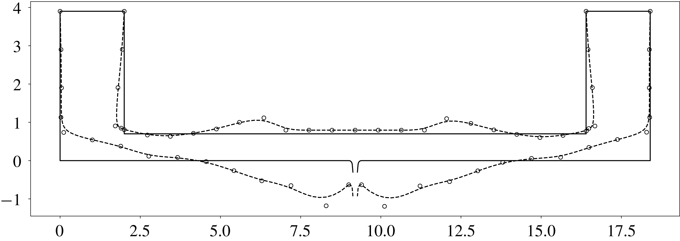
Figure 11. The initial (solid lines) and the optimized (dashed lines) printhead geometry. The inlet and the outlet boundaries remain fixed. The piezo-electric membrane and nozzle parts can move up and down but cannot change shape.
In this section we use the optimization algorithm in § 4.1.3 to update the control points until the relative improvement falls below the tolerance level of
 $\unicode[STIX]{x1D700}_{p}\leqslant 0.1$
. The optimized domain is shown in figure 11. The channel constricts near the corners of the top boundary, where the decay rate production had a local maximum. These constrictions increase the steady flow viscous dissipation there, but the central part of the channel expands to compensate. The new frequency of the first natural mode is
$\unicode[STIX]{x1D700}_{p}\leqslant 0.1$
. The optimized domain is shown in figure 11. The channel constricts near the corners of the top boundary, where the decay rate production had a local maximum. These constrictions increase the steady flow viscous dissipation there, but the central part of the channel expands to compensate. The new frequency of the first natural mode is
 $\text{Im}(s_{1}/2\unicode[STIX]{x03C0})=\unicode[STIX]{x1D714}/2\unicode[STIX]{x03C0}=0.264~\text{MHz}$
, and the decay rate increases to
$\text{Im}(s_{1}/2\unicode[STIX]{x03C0})=\unicode[STIX]{x1D714}/2\unicode[STIX]{x03C0}=0.264~\text{MHz}$
, and the decay rate increases to
 $\text{Re}(s_{1}/2\unicode[STIX]{x03C0})=\unicode[STIX]{x1D70E}/2\unicode[STIX]{x03C0}=0.0257~\text{MHz}$
, which is over 50 % higher than before. The steady flow viscous dissipation is the same as in the initial printhead. The parametric optimality coefficient of the optimized shape is
$\text{Re}(s_{1}/2\unicode[STIX]{x03C0})=\unicode[STIX]{x1D70E}/2\unicode[STIX]{x03C0}=0.0257~\text{MHz}$
, which is over 50 % higher than before. The steady flow viscous dissipation is the same as in the initial printhead. The parametric optimality coefficient of the optimized shape is
 $\unicode[STIX]{x1D6FC}_{p}=-0.94$
, showing that it is nearly optimal.
$\unicode[STIX]{x1D6FC}_{p}=-0.94$
, showing that it is nearly optimal.
Figure 12 shows the spatial distribution of the decay rate production
 $\ln (-\unicode[STIX]{x1D70E}_{\unicode[STIX]{x1D6FA}})$
inside the optimized domain. The viscous boundary layers overlap in the narrow parts of the channel, resulting in higher acoustic energy dissipation there. The highest amplitudes of decay rate production are around the nozzle. This shows that changes to the nozzle geometry are particularly influential.
$\ln (-\unicode[STIX]{x1D70E}_{\unicode[STIX]{x1D6FA}})$
inside the optimized domain. The viscous boundary layers overlap in the narrow parts of the channel, resulting in higher acoustic energy dissipation there. The highest amplitudes of decay rate production are around the nozzle. This shows that changes to the nozzle geometry are particularly influential.

Figure 12. Spatial distribution of the decay rate production absolute value in the optimized printhead channel (on a logarithmic scale),
 $\ln (-\unicode[STIX]{x1D70E}_{\unicode[STIX]{x1D6FA}})$
.
$\ln (-\unicode[STIX]{x1D70E}_{\unicode[STIX]{x1D6FA}})$
.
6 Conclusions
In this paper we perform constrained gradient-based shape optimization of a microchannel in an inkjet print head. Two Mach numbers are formed: one based on the steady flow and the other on the oscillating flow. Both Mach numbers are small, which allows us to separate the flow into (i) a steady flow with no oscillations (2.13) and (ii) oscillations with no steady flow (2.15). We then seek to control two objective functions by changing the shape of the boundaries. The objective functions are (i) the viscous dissipation of the first flow and (ii) a complex number that encapsulates the growth/decay rate and frequency of the second flow. We obtain expressions for the derivatives of the above objective functions with respect to boundary deformations in Hadamard form by deriving the adjoint equations for both flows.
These equations are general and could be used in many ways. We start by showing how they can be combined with an optimization algorithm in order to increase the viscous and thermal dissipation of oscillations in a channel without changing the viscous dissipation of the steady flow in the channel. This works by constricting the channel where the acoustic velocity is largest and enlarging the channel where the acoustic velocity is smallest. This result is straightforward and could have been obtained using physical intuition.
We then apply this technique to the same problem in a 2-D generic inkjet printhead. The printhead manufacturer would like to increase the decay rate of residual oscillations after a drop has been ejected, without changing the pressure drop required to continually flush ink through the head. Starting from a generic design and incorporating constraints such as the sizes of the nozzle and piezo-electric actuator, the algorithm converges to a design with a 50 % larger decay rate, but the same pressure drop, which we show to be nearly optimal. The final shape is not straightforward and would have been difficult to achieve through physical insight or trial and error. It could be improved further by adapting the parameters that describe the shape, but in this case the improvement would be small.
In this paper we derive and demonstrate a new way to optimize the shapes of channels that contain thermoviscous oscillating flows with (or without) steady flow. The main novelty is the cheap and accurate calculation of the shape gradients, using adjoint methods, which allows optimization with gradient-based algorithms. This is useful in two complementary ways. Firstly, these algorithms quickly converge to shapes that a human designer, using physical insight and trial and error, would probably not consider. Secondly, the adjoint methods provide physical insight into the mechanisms that influence the objective functions. It can be then used to alter the choice of shape parameters if it becomes apparent that the algorithm is missing a good shape due to a bad choice of shape parameters. The method in this paper is general and could be applied to many different applications in microfluidics. Its main requirements are that the steady flow Mach number and oscillating flow Mach number are small, and that dissipation is dominated by thermoviscous mechanisms.
Now that the technique has been proven on a 2-D geometry, the desirable next step is to apply it to 3-D geometries. For the adjoint methods and optimization algorithms, the extension from two to three dimensions is straightforward. For the shape parametrization, this extension is usually harder. In this case, however, the manufacturable 3-D shapes of inkjet print heads are severely constrained because they are etched into silicon wafers. Similar constraints apply to many microfluidic applications. These constraints, which require geometries to be close to two-dimensional, both render the 2-D analysis more relevant and make the 3-D shape parametrization more simple. Another extension, which is particularly relevant to inkjet printing, is to consider non-Newtonian fluids. Although these are challenging to model, it should be relatively straightforward to develop adjoints of these models. Another extension, which is the subject of our current work, is to use adjoint methods to optimize the droplet formation stage by varying the signal applied to the piezo-electric actuator.
Acknowledgements
We gratefully acknowledge the European Union’s Framework Programme for Research and Innovation Horizon 2020 under the Marie Skodowska-Curie Innovative Training Programme, H2020-MSCA-ITN-2015, for funding this project.
Appendix A
A.1 Derivation of the thermoviscous acoustic adjoint equations
The thermoviscous acoustic eigenvalue problem (2.20) can be written in terms of the velocity, pressure and temperature
 $\hat{\boldsymbol{q}}^{\text{T}}=(\hat{u} _{i},\hat{P},\hat{T})$
eigenvector and the complex eigenvalue
$\hat{\boldsymbol{q}}^{\text{T}}=(\hat{u} _{i},\hat{P},\hat{T})$
eigenvector and the complex eigenvalue
 $s$
in matrix form
$s$
in matrix form
 $sA\hat{\boldsymbol{q}}+B\hat{\boldsymbol{q}}=0$
:
$sA\hat{\boldsymbol{q}}+B\hat{\boldsymbol{q}}=0$
:
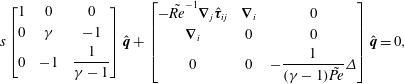 $$\begin{eqnarray}s\left[\begin{array}{@{}ccc@{}}1 & 0 & 0\\ 0 & \unicode[STIX]{x1D6FE} & -1\\ 0 & -1 & {\displaystyle \frac{1}{\unicode[STIX]{x1D6FE}-1}}\end{array}\right]\hat{\boldsymbol{q}}+\left[\begin{array}{@{}ccc@{}}-\tilde{Re}^{-1}\unicode[STIX]{x1D735}_{j}\hat{\unicode[STIX]{x1D749}}_{ij} & \unicode[STIX]{x1D735}_{i} & 0\\ \unicode[STIX]{x1D735}_{i} & 0 & 0\\ 0 & 0 & -{\displaystyle \frac{1}{(\unicode[STIX]{x1D6FE}-1)\tilde{Pe}}}\unicode[STIX]{x1D6E5}\end{array}\right]\hat{\boldsymbol{q}}=0,\end{eqnarray}$$
where
 $\hat{\unicode[STIX]{x1D749}}_{ij}$
denotes the viscous stress tensor differential operator,
$\hat{\unicode[STIX]{x1D749}}_{ij}$
denotes the viscous stress tensor differential operator,
 $\hat{\unicode[STIX]{x1D749}}_{ij}\hat{u} \equiv \hat{\unicode[STIX]{x1D70F}}_{ij}$
. The direct boundary conditions
$\hat{\unicode[STIX]{x1D749}}_{ij}\hat{u} \equiv \hat{\unicode[STIX]{x1D70F}}_{ij}$
. The direct boundary conditions
 ${\mathcal{N}}\hat{\boldsymbol{q}}=0$
satisfy the following equations:
${\mathcal{N}}\hat{\boldsymbol{q}}=0$
satisfy the following equations:
 $$\begin{eqnarray}\displaystyle & \displaystyle Z(s,x)\hat{u} _{i}=(-\hat{P}\unicode[STIX]{x1D6FF}_{ij}+\tilde{Re}^{-1}\hat{\unicode[STIX]{x1D70F}}_{ij})n_{j}, & \displaystyle\end{eqnarray}$$
 $$\begin{eqnarray}\displaystyle & \displaystyle \hat{T}=-\unicode[STIX]{x1D6FC}_{w}(s,x)\frac{\unicode[STIX]{x2202}\hat{T}}{\unicode[STIX]{x2202}n}. & \displaystyle\end{eqnarray}$$
There exists a corresponding adjoint state vector
 $\boldsymbol{q}^{+}=(u_{i}^{+},P^{+},T^{+})$
. We define the following volume and surface inner products:
$\boldsymbol{q}^{+}=(u_{i}^{+},P^{+},T^{+})$
. We define the following volume and surface inner products:
 $$\begin{eqnarray}\displaystyle & \displaystyle \langle \boldsymbol{a},\boldsymbol{b}\rangle =\int _{\unicode[STIX]{x1D6FA}}\boldsymbol{a}^{\ast }\boldsymbol{b}\,\text{d}\boldsymbol{x}, & \displaystyle\end{eqnarray}$$
 $$\begin{eqnarray}\displaystyle & \displaystyle \{\boldsymbol{a},\boldsymbol{b}\}=\int _{\unicode[STIX]{x2202}\unicode[STIX]{x1D6FA}}\boldsymbol{a}^{\ast }\boldsymbol{b}\,\text{d}s. & \displaystyle\end{eqnarray}$$
A Lagrangian functional of the system (A 1) with a objective function
 ${\mathcal{J}}$
is defined as
${\mathcal{J}}$
is defined as
 $$\begin{eqnarray}{\mathcal{L}}={\mathcal{J}}-\langle \boldsymbol{q}^{+},sA\hat{\boldsymbol{q}}+B\hat{\boldsymbol{q}}\rangle .\end{eqnarray}$$
The system’s eigenvalue sensitivity can be determined by setting
 ${\mathcal{J}}=s$
.
${\mathcal{J}}=s$
.
The optimality condition yields that the total variation of the Lagrangian with respect to the direct
 $\hat{\boldsymbol{q}},s$
, and the adjoint
$\hat{\boldsymbol{q}},s$
, and the adjoint
 $\boldsymbol{q}^{+}$
variables must be zero. The variation with respect to the adjoint variables gives the direct state equations. To determine the adjoint set of equations, we take the variation with respect to the direct variables and integrate the volume term in (A 4) by parts:
$\boldsymbol{q}^{+}$
variables must be zero. The variation with respect to the adjoint variables gives the direct state equations. To determine the adjoint set of equations, we take the variation with respect to the direct variables and integrate the volume term in (A 4) by parts:
 $$\begin{eqnarray}\frac{\unicode[STIX]{x2202}{\mathcal{L}}}{\unicode[STIX]{x2202}\hat{\boldsymbol{q}}}\unicode[STIX]{x1D6FF}\hat{\boldsymbol{q}}=0=\frac{\unicode[STIX]{x2202}{\mathcal{J}}}{\unicode[STIX]{x2202}\hat{\boldsymbol{q}}}\unicode[STIX]{x1D6FF}\hat{\boldsymbol{q}}-\langle s^{\ast }A^{+}\boldsymbol{q}^{+}+B^{+}\boldsymbol{q}^{+},\unicode[STIX]{x1D6FF}\hat{\boldsymbol{q}}\rangle -\{{\mathcal{N}}^{+}\boldsymbol{q}^{+},\unicode[STIX]{x1D6FF}\hat{\boldsymbol{q}}\}.\end{eqnarray}$$
The volume terms define the adjoint state equations, which in matrix form are:
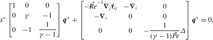 $$\begin{eqnarray}s^{\ast }\left[\begin{array}{@{}ccc@{}}1 & 0 & 0\\ 0 & \unicode[STIX]{x1D6FE} & -1\\ 0 & -1 & {\displaystyle \frac{1}{\unicode[STIX]{x1D6FE}-1}}\end{array}\right]\boldsymbol{q}^{+}+\left[\begin{array}{@{}ccc@{}}-\tilde{Re}^{-1}\unicode[STIX]{x1D735}_{j}\hat{\unicode[STIX]{x1D749}}_{ij} & -\unicode[STIX]{x1D735}_{i} & 0\\ -\unicode[STIX]{x1D735}_{i} & 0 & 0\\ 0 & 0 & -{\displaystyle \frac{1}{(\unicode[STIX]{x1D6FE}-1)\tilde{Pe}}}\unicode[STIX]{x1D6E5}\end{array}\right]\boldsymbol{q}^{+}=0,\end{eqnarray}$$
where
 $\hat{\unicode[STIX]{x1D749}}_{ij}\boldsymbol{q}^{+}=\unicode[STIX]{x1D70F}_{ij}^{+}\equiv \unicode[STIX]{x1D735}_{j}u_{i}^{+}+\unicode[STIX]{x1D735}_{i}u_{j}^{+}-2/3\unicode[STIX]{x1D6FF}_{ij}\,\text{div}\,u^{+}$
is the adjoint viscous stress tensor. The surface terms determine the adjoint boundary conditions
$\hat{\unicode[STIX]{x1D749}}_{ij}\boldsymbol{q}^{+}=\unicode[STIX]{x1D70F}_{ij}^{+}\equiv \unicode[STIX]{x1D735}_{j}u_{i}^{+}+\unicode[STIX]{x1D735}_{i}u_{j}^{+}-2/3\unicode[STIX]{x1D6FF}_{ij}\,\text{div}\,u^{+}$
is the adjoint viscous stress tensor. The surface terms determine the adjoint boundary conditions
 ${\mathcal{N}}^{+}\boldsymbol{q}^{+}=0$
:
${\mathcal{N}}^{+}\boldsymbol{q}^{+}=0$
:
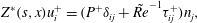 $$\begin{eqnarray}\displaystyle & \displaystyle Z^{\ast }(s,x)u_{i}^{+}=(P^{+}\unicode[STIX]{x1D6FF}_{ij}+\tilde{Re}^{-1}\unicode[STIX]{x1D70F}_{ij}^{+})n_{j}, & \displaystyle\end{eqnarray}$$
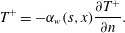 $$\begin{eqnarray}\displaystyle & \displaystyle T^{+}=-\unicode[STIX]{x1D6FC}_{w}(s,x)\frac{\unicode[STIX]{x2202}T^{+}}{\unicode[STIX]{x2202}n}. & \displaystyle\end{eqnarray}$$
Consideration of the direct (A 1) and adjoint (A 6) state equations, and the corresponding boundary conditions (A 2), (A 7) yields that the adjoint state can be expressed in terms of the direct state variables:
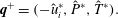 $$\begin{eqnarray}\boldsymbol{q}^{+}=(-\hat{u} _{i}^{\ast },\hat{P}^{\ast },\hat{T}^{\ast }).\end{eqnarray}$$
The variation of the Lagrangian with respect to the eigenvalue
 $\unicode[STIX]{x1D6FF}s$
gives the normalization condition:
$\unicode[STIX]{x1D6FF}s$
gives the normalization condition:
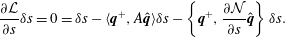 $$\begin{eqnarray}\frac{\unicode[STIX]{x2202}{\mathcal{L}}}{\unicode[STIX]{x2202}s}\unicode[STIX]{x1D6FF}s=0=\unicode[STIX]{x1D6FF}s-\langle \boldsymbol{q}^{+},A\hat{\boldsymbol{q}}\rangle \unicode[STIX]{x1D6FF}s-\left\{\boldsymbol{q}^{+},\frac{\unicode[STIX]{x2202}{\mathcal{N}}}{\unicode[STIX]{x2202}s}\hat{\boldsymbol{q}}\right\}\unicode[STIX]{x1D6FF}s.\end{eqnarray}$$
Taking into account the adjoint state representation in terms of the direct variables, the normalization condition is:
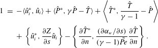 $$\begin{eqnarray}\displaystyle 1 & = & \displaystyle -\langle \hat{u} _{i}^{\ast },\hat{u} _{i}\rangle +\langle \hat{P}^{\ast },\unicode[STIX]{x1D6FE}\hat{P}-\hat{T}\rangle +\left\langle \hat{T}^{\ast },\frac{\hat{T}}{\unicode[STIX]{x1D6FE}-1}-\hat{P}\right\rangle \nonumber\\ \displaystyle & & \displaystyle +\,\left\{\hat{u} _{i}^{\ast },\frac{\unicode[STIX]{x2202}Z}{\unicode[STIX]{x2202}s}\hat{u} _{i}\right\}-\left\{\frac{\unicode[STIX]{x2202}\hat{T}^{\ast }}{\unicode[STIX]{x2202}n},\frac{(\unicode[STIX]{x2202}\unicode[STIX]{x1D6FC}_{w}/\unicode[STIX]{x2202}s)}{(\unicode[STIX]{x1D6FE}-1)\tilde{Pe}}\frac{\unicode[STIX]{x2202}\hat{T}}{\unicode[STIX]{x2202}n}\right\}.\end{eqnarray}$$
If the boundaries’ impedance and thermal accommodation coefficient are frequency independent, the surface terms in (A 10) vanish and the normalization condition is given by
 $$\begin{eqnarray}\langle \boldsymbol{q}^{+},A\hat{\boldsymbol{q}}\rangle =1.\end{eqnarray}$$
A.2 Oscillating flow shape sensitivity
We want to construct the eigenvalue shape sensitivity
 $G(\hat{\boldsymbol{q}},\boldsymbol{q}^{+})$
of the thermoviscous acoustic problem for a given shape displacement field
$G(\hat{\boldsymbol{q}},\boldsymbol{q}^{+})$
of the thermoviscous acoustic problem for a given shape displacement field
 $V$
. We take the variation of the Lagrangian (A 4) with respect to a shape perturbation
$V$
. We take the variation of the Lagrangian (A 4) with respect to a shape perturbation
 ${\mathcal{L}}^{\prime }[V]$
, and, due to the choice of the adjoint state (A 8), only the boundary terms do not vanish. This gives us the shape gradient
${\mathcal{L}}^{\prime }[V]$
, and, due to the choice of the adjoint state (A 8), only the boundary terms do not vanish. This gives us the shape gradient
 $$\begin{eqnarray}\displaystyle {\mathcal{L}}^{\prime }[V] & = & \displaystyle -\{{\mathcal{N}}^{+}\boldsymbol{q}^{+},\hat{\boldsymbol{q}}^{\prime }[V]\}=\{u_{i}^{+},(-\hat{P}^{\prime }[V]\unicode[STIX]{x1D6FF}_{ij}+\tilde{Re}^{-1}\hat{\unicode[STIX]{x1D70F}}_{ij}^{\prime }[V])n_{j}\}\nonumber\\ \displaystyle & & \displaystyle -\,\{(P^{+}\unicode[STIX]{x1D6FF}_{ij}+\tilde{Re}^{-1}\unicode[STIX]{x1D70F}_{ij}^{+})n_{j},\hat{u} _{i}^{\prime }[V]\}\nonumber\\ \displaystyle & & \displaystyle +\,\left\{T^{+},\frac{1}{(\unicode[STIX]{x1D6FE}-1)\tilde{Pe}}\frac{\unicode[STIX]{x2202}\hat{T}^{\prime }[V]}{\unicode[STIX]{x2202}n}\right\}-\left\{\frac{\unicode[STIX]{x2202}T^{+}}{\unicode[STIX]{x2202}n},\frac{1}{(\unicode[STIX]{x1D6FE}-1)\tilde{Pe}}\hat{T}^{\prime }[V]\right\}.\end{eqnarray}$$
For simplicity, we introduce the direct
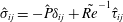 $\hat{\unicode[STIX]{x1D70E}}_{ij}=-\hat{P}\unicode[STIX]{x1D6FF}_{ij}+\tilde{Re}^{-1}\hat{\unicode[STIX]{x1D70F}}_{ij}$
and the adjoint
$\hat{\unicode[STIX]{x1D70E}}_{ij}=-\hat{P}\unicode[STIX]{x1D6FF}_{ij}+\tilde{Re}^{-1}\hat{\unicode[STIX]{x1D70F}}_{ij}$
and the adjoint
 $\unicode[STIX]{x1D70E}_{ij}^{+}=-P^{+}\unicode[STIX]{x1D6FF}_{ij}+\tilde{Re}^{-1}\unicode[STIX]{x1D70F}_{ij}^{+}$
force tensors. Also, we define the direct
$\unicode[STIX]{x1D70E}_{ij}^{+}=-P^{+}\unicode[STIX]{x1D6FF}_{ij}+\tilde{Re}^{-1}\unicode[STIX]{x1D70F}_{ij}^{+}$
force tensors. Also, we define the direct
 $\hat{q}_{i}=(1/(\unicode[STIX]{x1D6FE}-1)\tilde{Pe})\unicode[STIX]{x1D735}_{i}\hat{T}$
and adjoint
$\hat{q}_{i}=(1/(\unicode[STIX]{x1D6FE}-1)\tilde{Pe})\unicode[STIX]{x1D735}_{i}\hat{T}$
and adjoint
 $q_{i}^{+}=(1/(\unicode[STIX]{x1D6FE}-1)\tilde{Pe})\unicode[STIX]{x1D735}_{i}T^{+}$
heat fluxes, and their normal components
$q_{i}^{+}=(1/(\unicode[STIX]{x1D6FE}-1)\tilde{Pe})\unicode[STIX]{x1D735}_{i}T^{+}$
heat fluxes, and their normal components
 $\hat{q}_{i}n_{i}\equiv \hat{q}_{n}$
,
$\hat{q}_{i}n_{i}\equiv \hat{q}_{n}$
,
 $q_{i}^{+}n_{i}\equiv q_{n}^{+}$
.
$q_{i}^{+}n_{i}\equiv q_{n}^{+}$
.
On boundaries, the conditions (A 2) hold, resulting in the compliant and thermal boundary shape derivatives:
 $$\begin{eqnarray}\displaystyle 0=\text{d}(Z\hat{u} _{i}-\hat{\unicode[STIX]{x1D70E}}_{ij}n_{j})[V] & = & \displaystyle \text{d}Z[V]\hat{u} _{i}+Z\,\text{d}\hat{u} _{i}[V]-\text{d}\hat{\unicode[STIX]{x1D70E}}_{ij}[V]n_{j}-\hat{\unicode[STIX]{x1D70E}}_{ij}\,\text{d}n_{j}[V],\end{eqnarray}$$
 $$\begin{eqnarray}\displaystyle 0=\text{d}\left(\hat{T}+\unicode[STIX]{x1D6FC}_{w}\frac{\unicode[STIX]{x2202}\hat{T}}{\unicode[STIX]{x2202}n}\right)[V] & = & \displaystyle \text{d}\hat{T}[V]+\text{d}\unicode[STIX]{x1D6FC}_{w}[V]\frac{\unicode[STIX]{x2202}\hat{T}}{\unicode[STIX]{x2202}n}+\unicode[STIX]{x1D6FC}_{w}\,\text{d}n_{j}[V]\unicode[STIX]{x1D735}_{j}\hat{T}+\unicode[STIX]{x1D6FC}_{w}\frac{\unicode[STIX]{x2202}\,\text{d}\hat{T}[V]}{\unicode[STIX]{x2202}n}.\nonumber\\ \displaystyle & & \displaystyle\end{eqnarray}$$
 $$\begin{eqnarray}\displaystyle \text{d}\hat{u} _{i}[V] & = & \displaystyle \hat{u} _{i}^{\prime }[V]+(V\boldsymbol{\cdot }\unicode[STIX]{x1D735})\hat{u} _{i},\end{eqnarray}$$
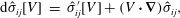 $$\begin{eqnarray}\displaystyle \text{d}\hat{\unicode[STIX]{x1D70E}}_{ij}[V] & = & \displaystyle \hat{\unicode[STIX]{x1D70E}}_{ij}^{\prime }[V]+(V\boldsymbol{\cdot }\unicode[STIX]{x1D735})\hat{\unicode[STIX]{x1D70E}}_{ij},\end{eqnarray}$$
 $$\begin{eqnarray}\displaystyle \text{d}\hat{T}[V] & = & \displaystyle \hat{T}^{\prime }[V]+(V\boldsymbol{\cdot }\unicode[STIX]{x1D735})\hat{T},\end{eqnarray}$$
 $$\begin{eqnarray}\displaystyle \text{d}(\unicode[STIX]{x1D735}_{j}\hat{T})[V] & = & \displaystyle \unicode[STIX]{x1D735}_{j}\hat{T}^{\prime }[V]+(V\boldsymbol{\cdot }\unicode[STIX]{x1D735})\unicode[STIX]{x1D735}_{j}\hat{T}.\end{eqnarray}$$
 $\text{d}Z[V]=0$
,
$\text{d}Z[V]=0$
,
 $\text{d}\unicode[STIX]{x1D6FC}_{w}[V]=0$
.
$\text{d}\unicode[STIX]{x1D6FC}_{w}[V]=0$
. The displacement vector field
 $V$
can be presented as a sum of its normal and tangential components,
$V$
can be presented as a sum of its normal and tangential components,
 $V=(V\boldsymbol{\cdot }\boldsymbol{n})\boldsymbol{n}+\sum _{i=1}^{d-1}(V\boldsymbol{\cdot }\unicode[STIX]{x1D749}_{i})\unicode[STIX]{x1D749}_{i}$
, where
$V=(V\boldsymbol{\cdot }\boldsymbol{n})\boldsymbol{n}+\sum _{i=1}^{d-1}(V\boldsymbol{\cdot }\unicode[STIX]{x1D749}_{i})\unicode[STIX]{x1D749}_{i}$
, where
 $\unicode[STIX]{x1D749}_{i}$
spans the (
$\unicode[STIX]{x1D749}_{i}$
spans the (
 $d-1$
)-dimensional space tangent to the surface. As shown in Sokolowski & Zolesio (Reference Sokolowski and Zolesio1992), a shape derivative vanishes in the tangential direction, since any boundary deformation in the tangential direction does not change the domain boundary. Therefore, for a domain boundary of sufficient smoothness the shape derivatives in the direction of the displacement field are equivalent to the shape derivatives in its normal projection. Therefore
$d-1$
)-dimensional space tangent to the surface. As shown in Sokolowski & Zolesio (Reference Sokolowski and Zolesio1992), a shape derivative vanishes in the tangential direction, since any boundary deformation in the tangential direction does not change the domain boundary. Therefore, for a domain boundary of sufficient smoothness the shape derivatives in the direction of the displacement field are equivalent to the shape derivatives in its normal projection. Therefore
 $V$
can be replaced with
$V$
can be replaced with
 $(V\boldsymbol{\cdot }\boldsymbol{n})\boldsymbol{n}$
and
$(V\boldsymbol{\cdot }\boldsymbol{n})\boldsymbol{n}$
and
 $(V\boldsymbol{\cdot }\unicode[STIX]{x1D735})$
with
$(V\boldsymbol{\cdot }\unicode[STIX]{x1D735})$
with
 $(V\boldsymbol{\cdot }\boldsymbol{n})\unicode[STIX]{x2202}/\unicode[STIX]{x2202}\boldsymbol{n}$
. By introducing the tangential gradient
$(V\boldsymbol{\cdot }\boldsymbol{n})\unicode[STIX]{x2202}/\unicode[STIX]{x2202}\boldsymbol{n}$
. By introducing the tangential gradient
 $\unicode[STIX]{x1D735}_{i}^{\unicode[STIX]{x1D6E4}}=\unicode[STIX]{x1D735}_{i}-n_{i}n_{j}\unicode[STIX]{x1D735}_{j}$
, the shape derivative of the boundary normal is (Sonntag, Schmidt & Gauger Reference Sonntag, Schmidt and Gauger2016)
$\unicode[STIX]{x1D735}_{i}^{\unicode[STIX]{x1D6E4}}=\unicode[STIX]{x1D735}_{i}-n_{i}n_{j}\unicode[STIX]{x1D735}_{j}$
, the shape derivative of the boundary normal is (Sonntag, Schmidt & Gauger Reference Sonntag, Schmidt and Gauger2016)
 $$\begin{eqnarray}\text{d}n_{i}[V]=-\unicode[STIX]{x1D735}_{i}^{\unicode[STIX]{x1D6E4}}(V\boldsymbol{\cdot }\boldsymbol{n}).\end{eqnarray}$$
Combining (A 13)–(A 15), the shape derivatives of the compliant boundary condition and the thermal boundary condition result in
 $$\begin{eqnarray}\displaystyle Z\hat{u} _{i}^{\prime }[V]-\hat{\unicode[STIX]{x1D70E}}_{ij}^{\prime }[V]n_{j} & = & \displaystyle -Z(V\boldsymbol{\cdot }\boldsymbol{n})\frac{\unicode[STIX]{x2202}\hat{u} _{i}}{\unicode[STIX]{x2202}n}+(V\boldsymbol{\cdot }\boldsymbol{n})n_{j}\frac{\unicode[STIX]{x2202}\hat{\unicode[STIX]{x1D70E}}_{ij}}{\unicode[STIX]{x2202}n}-\hat{\unicode[STIX]{x1D70E}}_{ij}\unicode[STIX]{x1D735}_{i}^{\unicode[STIX]{x1D6E4}}(V\boldsymbol{\cdot }\boldsymbol{n}),\end{eqnarray}$$
 $$\begin{eqnarray}\displaystyle \hat{T}^{\prime }[V]+\unicode[STIX]{x1D6FC}_{w}\frac{\unicode[STIX]{x2202}\hat{T}^{\prime }[V]}{\unicode[STIX]{x2202}n} & = & \displaystyle -(V\boldsymbol{\cdot }\boldsymbol{n})\frac{\unicode[STIX]{x2202}\hat{T}}{\unicode[STIX]{x2202}n}-\unicode[STIX]{x1D6FC}_{w}(V\boldsymbol{\cdot }\boldsymbol{n})n_{j}\frac{\unicode[STIX]{x2202}\unicode[STIX]{x1D735}_{j}\hat{T}}{\unicode[STIX]{x2202}n}+\unicode[STIX]{x1D6FC}_{w}\unicode[STIX]{x1D735}_{i}^{\unicode[STIX]{x1D6E4}}(V\boldsymbol{\cdot }\boldsymbol{n})\unicode[STIX]{x1D735}_{i}\hat{T}.\qquad\end{eqnarray}$$
 $$\begin{eqnarray}\displaystyle {\mathcal{L}}^{\prime }[V] & = & \displaystyle \{u_{i}^{+},\hat{\unicode[STIX]{x1D70E}}_{ij}^{\prime }[V]n_{j}-Z\hat{u} _{i}^{\prime }[V]\}-\left\{q_{n}^{+},\hat{T}^{\prime }[V]+\unicode[STIX]{x1D6FC}_{w}\frac{\unicode[STIX]{x2202}\hat{T}^{\prime }[V]}{\unicode[STIX]{x2202}n}\right\}\end{eqnarray}$$
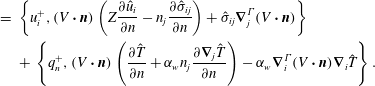 $$\begin{eqnarray}\displaystyle & = & \displaystyle \left\{u_{i}^{+},(V\boldsymbol{\cdot }\boldsymbol{n})\left(Z\frac{\unicode[STIX]{x2202}\hat{u} _{i}}{\unicode[STIX]{x2202}n}-n_{j}\frac{\unicode[STIX]{x2202}\hat{\unicode[STIX]{x1D70E}}_{ij}}{\unicode[STIX]{x2202}n}\right)+\hat{\unicode[STIX]{x1D70E}}_{ij}\unicode[STIX]{x1D735}_{j}^{\unicode[STIX]{x1D6E4}}(V\boldsymbol{\cdot }\boldsymbol{n})\right\}\nonumber\\ \displaystyle & & \displaystyle +\,\left\{q_{n}^{+},(V\boldsymbol{\cdot }\boldsymbol{n})\left(\frac{\unicode[STIX]{x2202}\hat{T}}{\unicode[STIX]{x2202}n}+\unicode[STIX]{x1D6FC}_{w}n_{j}\frac{\unicode[STIX]{x2202}\unicode[STIX]{x1D735}_{j}\hat{T}}{\unicode[STIX]{x2202}n}\right)-\unicode[STIX]{x1D6FC}_{w}\unicode[STIX]{x1D735}_{i}^{\unicode[STIX]{x1D6E4}}(V\boldsymbol{\cdot }\boldsymbol{n})\unicode[STIX]{x1D735}_{i}\hat{T}\right\}.\end{eqnarray}$$
 $A$
and a scalar field
$A$
and a scalar field
 $b$
:
$b$
: 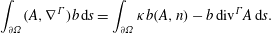 $$\begin{eqnarray}\int _{\unicode[STIX]{x2202}\unicode[STIX]{x1D6FA}}(A,\unicode[STIX]{x1D6FB}^{\unicode[STIX]{x1D6E4}})b\,\text{d}s=\int _{\unicode[STIX]{x2202}\unicode[STIX]{x1D6FA}}\unicode[STIX]{x1D705}b(A,n)-b\,\text{div}^{\unicode[STIX]{x1D6E4}}A\,\text{d}s.\end{eqnarray}$$
Here
 $\unicode[STIX]{x1D705}=\text{div}^{\unicode[STIX]{x1D6E4}}n$
describes the surface curvature. With
$\unicode[STIX]{x1D705}=\text{div}^{\unicode[STIX]{x1D6E4}}n$
describes the surface curvature. With
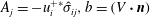 $A_{j}=-u_{i}^{+\ast }\hat{\unicode[STIX]{x1D70E}}_{ij},b=(V\boldsymbol{\cdot }\boldsymbol{n})$
, the transformation of the stress contribution (the first surface integral in (A 17b
)) to Hadamard form is given by
$A_{j}=-u_{i}^{+\ast }\hat{\unicode[STIX]{x1D70E}}_{ij},b=(V\boldsymbol{\cdot }\boldsymbol{n})$
, the transformation of the stress contribution (the first surface integral in (A 17b
)) to Hadamard form is given by
 $$\begin{eqnarray}u_{i}^{+\ast }\hat{\unicode[STIX]{x1D70E}}_{ij}\unicode[STIX]{x1D735}_{j}^{\unicode[STIX]{x1D6E4}}(V\boldsymbol{\cdot }\boldsymbol{n})=\unicode[STIX]{x1D705}(V\boldsymbol{\cdot }\boldsymbol{n})u_{i}^{+\ast }\hat{\unicode[STIX]{x1D70E}}_{ij}n_{j}-(V\boldsymbol{\cdot }\boldsymbol{n})\unicode[STIX]{x1D735}_{j}^{\unicode[STIX]{x1D6E4}}(u_{i}^{+\ast }\hat{\unicode[STIX]{x1D70E}}_{ij}),\end{eqnarray}$$
and using the definition of the tangential gradient, the tangential divergence in (A 19) combines with the following term and we obtain:
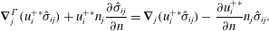 $$\begin{eqnarray}\unicode[STIX]{x1D735}_{j}^{\unicode[STIX]{x1D6E4}}(u_{i}^{+\ast }\hat{\unicode[STIX]{x1D70E}}_{ij})+u_{i}^{+\ast }n_{j}\frac{\unicode[STIX]{x2202}\hat{\unicode[STIX]{x1D70E}}_{ij}}{\unicode[STIX]{x2202}n}=\unicode[STIX]{x1D735}_{j}(u_{i}^{+\ast }\hat{\unicode[STIX]{x1D70E}}_{ij})-\frac{\unicode[STIX]{x2202}u_{i}^{+\ast }}{\unicode[STIX]{x2202}n}n_{j}\hat{\unicode[STIX]{x1D70E}}_{ij}.\end{eqnarray}$$
For the thermal contribution (the second surface integral in (A 17b
))
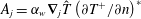 $A_{j}=\unicode[STIX]{x1D6FC}_{w}\unicode[STIX]{x1D735}_{j}\hat{T}\left(\unicode[STIX]{x2202}T^{+}/\unicode[STIX]{x2202}n\right)^{\ast }$
so the Hadamard form is:
$A_{j}=\unicode[STIX]{x1D6FC}_{w}\unicode[STIX]{x1D735}_{j}\hat{T}\left(\unicode[STIX]{x2202}T^{+}/\unicode[STIX]{x2202}n\right)^{\ast }$
so the Hadamard form is:
 $$\begin{eqnarray}\displaystyle & & \displaystyle \unicode[STIX]{x1D6FC}_{w}q_{n}^{+}\unicode[STIX]{x1D735}_{j}\hat{T}\unicode[STIX]{x1D735}_{j}^{\unicode[STIX]{x1D6E4}}(V\boldsymbol{\cdot }\boldsymbol{n})\nonumber\\ \displaystyle & & \displaystyle \quad =\unicode[STIX]{x1D705}(V\boldsymbol{\cdot }\boldsymbol{n})\unicode[STIX]{x1D6FC}_{w}q_{n}^{+\ast }\frac{\unicode[STIX]{x2202}\hat{T}}{\unicode[STIX]{x2202}n}-(V\boldsymbol{\cdot }\boldsymbol{n})\unicode[STIX]{x1D735}_{j}^{\unicode[STIX]{x1D6E4}}(\unicode[STIX]{x1D6FC}_{w}q_{n}^{+\ast }\unicode[STIX]{x1D735}_{j}\hat{T})\nonumber\\ \displaystyle & & \displaystyle \quad =(V\boldsymbol{\cdot }\boldsymbol{n})\left(\unicode[STIX]{x1D705}\unicode[STIX]{x1D6FC}_{w}q_{n}^{+\ast }\frac{\unicode[STIX]{x2202}\hat{T}}{\unicode[STIX]{x2202}n}-\unicode[STIX]{x1D6FC}_{w}q_{n}^{+\ast }\left(\unicode[STIX]{x0394}\hat{T}-n_{j}\frac{\unicode[STIX]{x2202}\unicode[STIX]{x1D735}_{j}\hat{T}}{\unicode[STIX]{x2202}n}\right)-\unicode[STIX]{x1D735}_{j}^{\unicode[STIX]{x1D6E4}}(\unicode[STIX]{x1D6FC}_{w}q_{n}^{+\ast })\unicode[STIX]{x1D735}_{j}^{\unicode[STIX]{x1D6E4}}\hat{T}\right)\!.\qquad\end{eqnarray}$$
After rearranging the terms in (A 17), the shape derivative in Hadamard form is given by the surface integral of the normal displacement and the sum of the stress and thermal sensitivity functionals,
 $G_{s}^{str}$
and
$G_{s}^{str}$
and
 $G_{s}^{th}$
:
$G_{s}^{th}$
:
 $$\begin{eqnarray}s^{\prime }[V]={\mathcal{L}}^{\prime }[V]=\int _{\unicode[STIX]{x2202}\unicode[STIX]{x1D6FA}}(V\boldsymbol{\cdot }\boldsymbol{n})(G_{s}^{str}(\hat{\boldsymbol{q}},\boldsymbol{q}^{+})+G_{s}^{th}(\hat{\boldsymbol{q}},\boldsymbol{q}^{+})),\end{eqnarray}$$
where the functionals are defined as
 $$\begin{eqnarray}\displaystyle G_{s}^{str}(\hat{\boldsymbol{q}},\boldsymbol{q}^{+}) & = & \displaystyle \frac{\unicode[STIX]{x2202}\hat{u} _{i}}{\unicode[STIX]{x2202}n}n_{j}\unicode[STIX]{x1D70E}_{ij}^{+\ast }+\frac{\unicode[STIX]{x2202}u_{i}^{+\ast }}{\unicode[STIX]{x2202}n}n_{j}\hat{\unicode[STIX]{x1D70E}}_{ij}+\unicode[STIX]{x1D705}\hat{u} _{i}\unicode[STIX]{x1D70E}_{ij}^{+\ast }n_{j}-\unicode[STIX]{x1D735}_{j}(u_{i}^{+\ast }\hat{\unicode[STIX]{x1D70E}}_{ij}),\end{eqnarray}$$
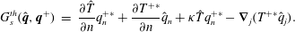 $$\begin{eqnarray}\displaystyle G_{s}^{th}(\hat{\boldsymbol{q}},\boldsymbol{q}^{+}) & = & \displaystyle \frac{\unicode[STIX]{x2202}\hat{T}}{\unicode[STIX]{x2202}n}q_{n}^{+\ast }+\frac{\unicode[STIX]{x2202}T^{+\ast }}{\unicode[STIX]{x2202}n}\hat{q}_{n}+\unicode[STIX]{x1D705}\hat{T}q_{n}^{+\ast }-\unicode[STIX]{x1D735}_{j}(T^{+\ast }\hat{q}_{j}).\end{eqnarray}$$
Finally, considering (A 8), the eigenvalue sensitivity functionals can be derived:
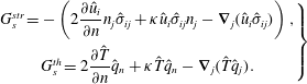 $$\begin{eqnarray}\left.\begin{array}{@{}c@{}}G_{s}^{str}=-\left(2{\displaystyle \frac{\unicode[STIX]{x2202}\hat{u} _{i}}{\unicode[STIX]{x2202}n}}n_{j}\hat{\unicode[STIX]{x1D70E}}_{ij}+\unicode[STIX]{x1D705}\hat{u} _{i}\hat{\unicode[STIX]{x1D70E}}_{ij}n_{j}-\unicode[STIX]{x1D735}_{j}(\hat{u} _{i}\hat{\unicode[STIX]{x1D70E}}_{ij})\right),\\ G_{s}^{th}=2{\displaystyle \frac{\unicode[STIX]{x2202}\hat{T}}{\unicode[STIX]{x2202}n}}\hat{q}_{n}+\unicode[STIX]{x1D705}\hat{T}\hat{q}_{n}-\unicode[STIX]{x1D735}_{j}(\hat{T}\hat{q}_{j}).\end{array}\right\}\end{eqnarray}$$
Two special cases, the no-slip and stress-free boundaries, simplify the viscous sensitivity functional to
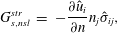 $$\begin{eqnarray}\displaystyle G_{s,nsl}^{str} & = & \displaystyle -\frac{\unicode[STIX]{x2202}\hat{u} _{i}}{\unicode[STIX]{x2202}n}n_{j}\hat{\unicode[STIX]{x1D70E}}_{ij},\end{eqnarray}$$
 $$\begin{eqnarray}\displaystyle G_{s,free}^{str} & = & \displaystyle \unicode[STIX]{x1D735}_{j}(\hat{u} _{i}\hat{\unicode[STIX]{x1D70E}}_{ij}),\end{eqnarray}$$
 $$\begin{eqnarray}\displaystyle G_{s,iso}^{th} & = & \displaystyle \frac{\unicode[STIX]{x2202}\hat{T}}{\unicode[STIX]{x2202}n}\hat{q}_{n},\end{eqnarray}$$
 $$\begin{eqnarray}\displaystyle G_{s,ad}^{th} & = & \displaystyle -\unicode[STIX]{x1D735}_{j}(\hat{T}\hat{q}_{j}).\end{eqnarray}$$