


1 Introduction
Subjects in laboratory experiments consistently deviate from equilibrium behavior (Camerer Reference Camerer2003). Many models of bounded rationality try to explain these deviations through errors in belief formation (e.g., Nagel Reference Nagel1995; Ho et al. Reference Ho, Camerer and Weigelt1998; Weizsäcker Reference Weizsäcker2003). Another explanation is that subjects fail to fully understand the structure of the game (Chou et al. Reference Chou, McConnell, Nagel and Plott2009 refer to this as an absence of “game form recognition”). Generally, when analyzing deviations from equilibrium behavior, one would expect both of these effects to play a role. However it is typically hard (if not impossible) to distinguish between the two, as correct belief formation crucially depends on a correct understanding of the structure of the game. With the help of a novel one-player guessing game experiment, we are able to disentangle these two effects, thus improving the understanding of why subjects deviate from equilibrium behavior.
An extensive literature has attempted to analyze both belief formation and understanding the structure of the game. Costa-Gomes and Crawford (Reference Costa-Gomes and Crawford2006) present subjects with a series of two-player dominance-solvable games and conclude that most subjects understand the games, but play non-equilibrium strategies due to their “simplified models of others’ decisions.” In Costa-Gomes and Weizsäcker (Reference Costa-Gomes and Weizsäcker2008) the authors look at subject’s actions and their stated beliefs, and find that subjects rarely best respond to their stated beliefs. However, Rey-Biel (Reference Rey-Biel2009) observes that in simplified versions of the games studied in Costa-Gomes and Weizsäcker (Reference Costa-Gomes and Weizsäcker2008), Nash Equilibrium is a better predictor of subject behavior than any other model based on level-K reasoning.
Another strand of the literature focuses on whether subjects understand the structure of the game. Using two-player guessing games, Chou et al. (Reference Chou, McConnell, Nagel and Plott2009) find that subjects are surprisingly unable to understand the experimental setup they are participating in. By using different sets of instructions for the same game, and by introducing hints, they show that subjects do not deviate from equilibrium because of cognitive biases, but rather because of a lack of game form recognition, which they define as the relationships between possible choices, outcomes, and payoffs. Fragiadakis et al. (Reference Fragiadakis, Knoepfle and Niederle2016) let subjects play a two-player guessing game repeatedly against random opponents, and subsequently ask subjects to replicate or best respond to their previous choices. They find that while behavior of only 30% of subjects is consistent with a set of commonly used models (including equilibrium play and level-K), they also identify subjects who play strategically but are not identified by commonly used models. Finally, Agranov et al. (Reference Agranov, Caplin and Tergiman2015) develop an experimental protocol that allows them to track the decision-making process of subjects in a beauty contest game. The results show that around 45% of subjects consider playing weakly dominated strategies at some point in their decision-making process.
In this experiment, we use a one-player guessing game which allows to measure how well subjects understand the structure of the two-player guessing game (Grosskopf and Nagel Reference Grosskopf and Nagel2008). In this “game” subjects play the role of both players in a two-player guessing game. That is, they are asked to pick not one but two numbers between 0 and 100, and are paid according to the proximity of each of their choices to two thirds of the average of both choices. This setup switches off the belief channel, but still demands subjects to understand the structure of the game.Footnote 1 By comparing their actions in a two-player guessing game to the choices made in the one-player guessing game we can disentangle the effects of beliefs from “game form recognition,” and analyze to what extent understanding the structure of the game determines their belief formation and their best-responses.Footnote 2
Our experimental results show that a majority of subjects fails to fully solve the one-player guessing game, and that subjects with a better understanding of the structure of the one-player guessing game play values closer the Nash Equilibrium in the two-player guessing game. This implies that an important part of non-equilibrium play is likely due to the inability of subjects to fully understand the structure of the game. Additionally, we observe that subjects with a better understanding of the one-player guessing game form more accurate beliefs, are better at best-responding to their own beliefs, and tend to better adjust their beliefs according to the population they face. These results confirm the intuition that understanding the structure of the game is crucial for belief formation.
2 Experimental design
The experiment consists of four different parts: Subjects first play the one-player guessing game (1PG), followed by the two-player guessing game (2PG). After this, we elicit subjects’ beliefs about other subjects’ two-player guessing game choices. A subset of subjects then participated in an additional belief elicitaton task (“What-if” belief elicitation). At the end of the experiment, all subjects are asked to answer a battery of cognitive ability tests. In the following we describe each part of the experiment in more detail.
2.1 The one-player guessing game (1PG)
The one-player guessing game, first introduced in Bosch-Rosa et al. (Reference Bosch-Rosa, Meissner and Bosch-Domènech2018), allows to test whether subjects can solve the two-player guessing game introduced by Grosskopf and Nagel (Reference Grosskopf and Nagel2008) free of any strategic concerns.Footnote 3
In essence, subjects play the role of both players in a two-player guessing game, i.e. they play the two player guessing game “against themselves.” Accordingly, each subject (i) picks two numbers
 and
and
 and is paid depending on the absolute distance of each chosen number to the “target value” which is two thirds of the average of both numbers. The further away each chosen number is from this target value, the lower is the payoff. Formally the experimental payoff for choosing number
 and
and
 is:
is:
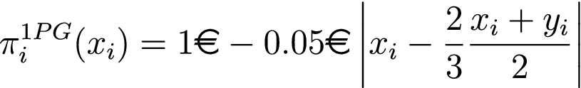
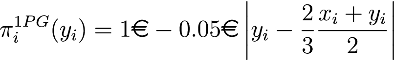
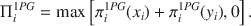
Subjects are paid for both choices, so their combined payoff is:
The payoff function is maximized at
 . This solution can be found through logical induction by starting with a random value
 , and then calculating the “best response” which is
 . Following this, a “best response to the best response” can be calculated (
 ) and so on until reaching the fixed point (
 ,
,
 ).
).
By turning the two-player guessing game into an algebraic problem with no strategic uncertainty, we can separate those subjects who can solve the mathematical problem associated with the guessing game from those who cannot.Footnote 4
2.2 The two-player guessing game (2PG)
The two-player guessing game that we use is an adaptation of the one presented in Grosskopf and Nagel (Reference Grosskopf and Nagel2008) and Nagel et al. (Reference Nagel, Bühren and Frank2016). Subjects are matched in pairs and asked to simultaneously pick a number
 . In Grosskopf and Nagel (Reference Grosskopf and Nagel2008) the winner is whoever picks the number closer to 2/3 of the average of both numbers, so unlike in games with
 subjects, now
 is a (unique) weakly dominant strategy. In our version of the 2PG, the payments are based on the (absolute) distance of each individual pick to 2/3 of the average of both numbers. Formally, the payment for player i depends on the choices of player j and her own in the following way:Footnote 5
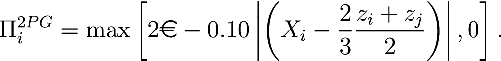
This small change in payoffs dramatically changes the game as now the equilibrium is reached through iterated deletion of strictly dominated strategies, and zero is no longer a weakly dominant strategy. Now the best response is to choose 1/2 of the number a player believes the other player chooses.Footnote 6
We opted for this modification of the original game for two reasons. First, it allows us to de facto ask subjects for a point estimate of their belief about the other subject’s choice, and secondly, and more important, it makes the game comparable to the 1PG. Note that while certainly not standard, distance-based payoff structures are widely used in the literature. Güth et al. (Reference Güth, Kocher and Sutter2002) first utilized such a payoff structure, arguing that it more closely resembles the financial decision-making situations that beauty contests are often intended to emulate. Since then a number of experiments have used distance-based beauty contests.Footnote 7 Most relevant for our experiment is Nagel et al. (Reference Nagel, Bühren and Frank2016), who directly compare distance-based and tournament incentives in two player guessing games and find no significant differences across the choices of subjects.
2.3 Belief elicitation
After subjects had played the 1PG and the 2PG (with no feedback in both cases) we elicited their beliefs about the other players’ decisions in the 2PG. Similar to Lahav (Reference Lahav2015), subjects were asked to distribute a total of 19 “tokens” into 20 “bins”.
Each token represented a subject in the session (each session consisted of 20 subjects), and each bin had a range of 4 integers that players could play in the 2PG (i.e. the first bin had the range [0,4], the second [5,9], and so on). See Fig. 11 in "Electronic supplementary material Appendix C" for a screen-shot of the experimental interface.
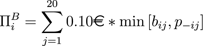
To incentivize subjects, we used a linear scoring rule that paid €0.10 for each token that overlapped with the choice of any other subject in the 2PG. For instance, if a subject put three tokens in the bin “5–9” and in her session only 2 subjects had actually played any value within this range, then she would receive a total of 20 cents for the tokens allocated in that bin. If, on the other hand, she placed 5 token in the bin “0–4” and 10 subjects had played a value in this range, then she would be paid 50 cents for the tokens allocated in that bin.
Formally, define
 as the number of tokens that subject i deposited in bin j, and
 as the number of subjects other than player i that chose a value that falls within bin j in the 2PG. Then the payoff for belief formation for subject i is:
The resulting distribution of beliefs provides an estimate of what subjects think about other subjects’ choices, and allows us to analyze how subject best-respond to their own beliefs.Footnote 8
2.3.1 “What if” belief elicitation
Since playing the 1PG could have an influence on the beliefs subjects form in the 2PG, we asked a subset of 40 subjects to additionally guess the choices of players in a 2PG who had not previously taken part in the 1PG.Footnote 9 The incentives for this elicitation task are the same as the ones described above, and the data came from a random pick of 19 subjects from a sample of 80 subjects who we had invited two weeks earlier to participate in a 2PG without previously taking part in the 1PG.
2.4 Cognitive ability
Gill and Prowse (Reference Gill and Prowse2016) show that subjects who score higher in a Raven Test (Raven Reference Raven1960) choose numbers closer to equilibrium, earn more, and converge quicker to equilibrium in a three-player guessing game.Footnote 10 Since we are interested in studying the ability of subjects to solve the guessing game, we also tested the cognitive ability of our subjects. In particular, all subjects answered a Raven Test and played “Race-to-60,” a variant of the Race game (see e.g. Gneezy et al. Reference Gneezy, Rustichini and Vostroknutov2010; Levitt et al. Reference Levitt, List and Sally2011).Footnote 11 The Raven Test is a multiple choice test in which subjects must pick an element that best completes a missing element in a matrix of geometrical shapes (see an example in Fig. 12 of "Electronic supplementary material Appendix C"). The score of this test has been found to correlate with measures of strategic sophistication and the ability of subjects to solve novel problems (Carpenter et al. Reference Carpenter, Just and Shell1990). It is increasingly used in economic research due to its simplicity and the lack of required technical skills.
Since logical induction is a central element of the guessing games, we test this ability with the “Race-to-60” game. In this game, each participant and a computerized player sequentially choose numbers between 1 and 10, which are added up. Whoever is first to push the sum to or above 60 wins the game. The game is solvable by backward induction, and the first mover can always win by picking numbers such that the common pool adds up to the sequence : [5; 16; 27; 38; 49; 60]. Subjects always move first and therefore, independent of the computer’s backward induction ability, can always win the game.Footnote 12
3 Results
A total of 80 subjects participated in this experiment. All subjects were recruited through ORSEE (Greiner Reference Greiner2015) and were mostly undergraduate students with a variety of backgrounds, ranging from anthropology to electrical engineering or architecture. Sessions lasted one and a half hours and were run at the Experimental Economics Laboratory of the Technische Universität Berlin. Subjects who had previously participated in guessing game experiments were not invited. The experiment was programmed and conducted using z-Tree (Fischbacher Reference Fischbacher2007). For detailed results on the cognitive ability tests, see "Electronic supplementary material Appendix A"
3.1 The one player guessing game
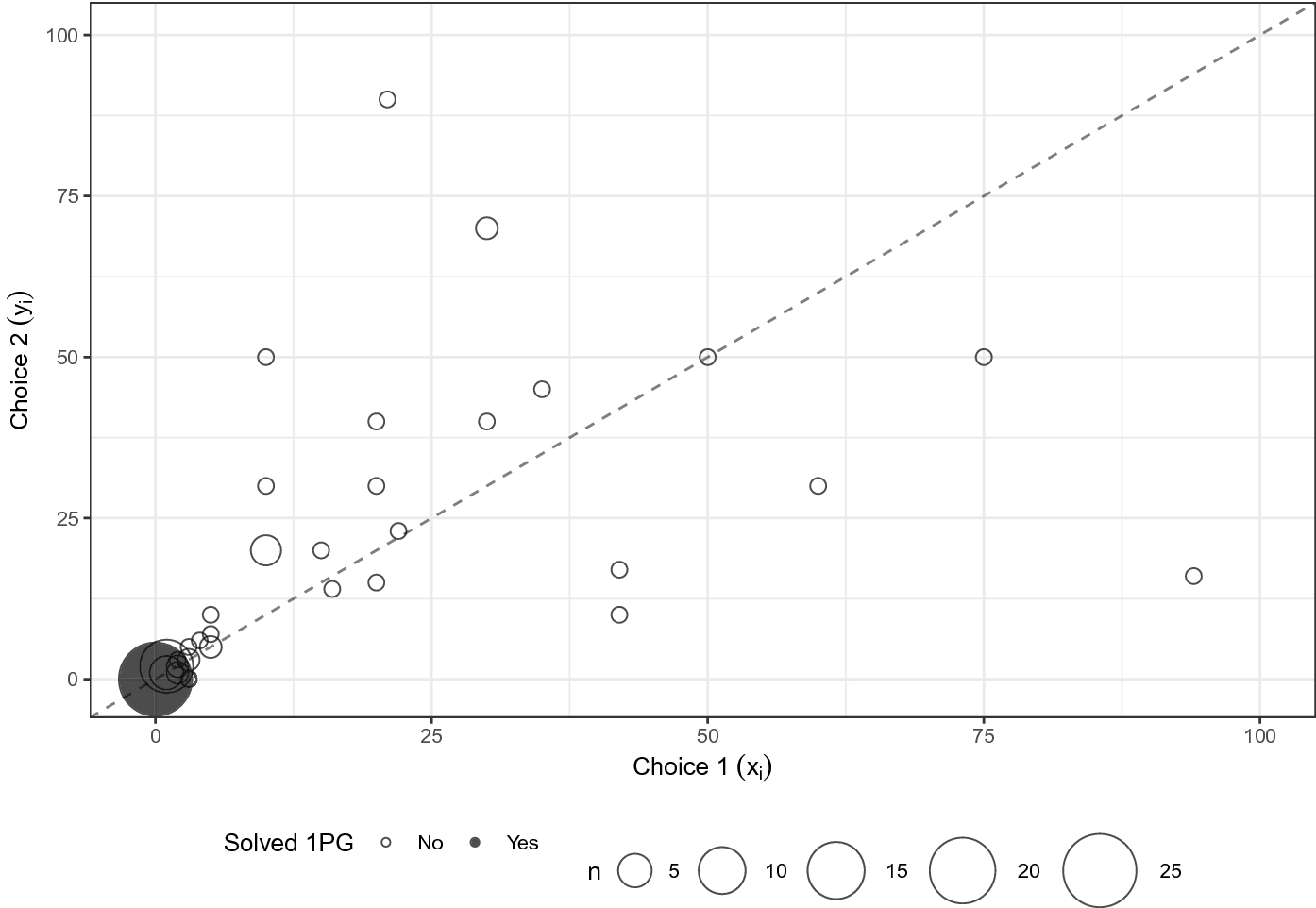
Fig. 1 Scatter plot of the choices made by each subject. Darker dots refer to subjects that fully solved the game (0,0). See Fig. 13 in "Electronic supplementary material Appendix C" for a zoom in plot depicting only the choices from [0,50]
In Fig. 1 we present the results of the 1PG in a scatter plot. Recall that in this case subjects have to pick two numbers,
 ; the first number is depicted on the horizontal axis, the second on the vertical axis. The diagonal dashed line marks the points where a subject picked the same number for
 and
and
 . The solid circle indicates subjects who fully solved the game (0,0).
As can be seen, only a minority (
 ) of subjects is able to fully solve the 1PG, i.e., pick zero for both numbers. In the remainder of this paper we will use this ability to fully solve the game as our primary measure of understanding of the structure of the guessing game.
Result 1
Only 31% of our subjects fully understand the one-player guessing game.
Another interesting observation in Fig. 1 is that subjects who play numbers closer together also play numbers closer to the origin. This is relevant, as in the 1PG there are two ways in which a subject (who has not fully solved the game) can improve her payoffs: by picking numbers closer to zero, and/or by picking numbers that are closer to each other. A Spearman test confirms the correlation between higher average of both choices and the distance between them (Spearman
 , p value
 ). As subjects with high payoffs played both numbers that were close to each other, and to zero, one could interpret the payoffs of the 1PG as a measure of (partial) understanding of the structure of the guessing game. Therefore, we will use the payoffs of the 1PG as a secondary measure to complement to our primary measure of understanding, “Solved 1PG”/“Not solved 1PG”.
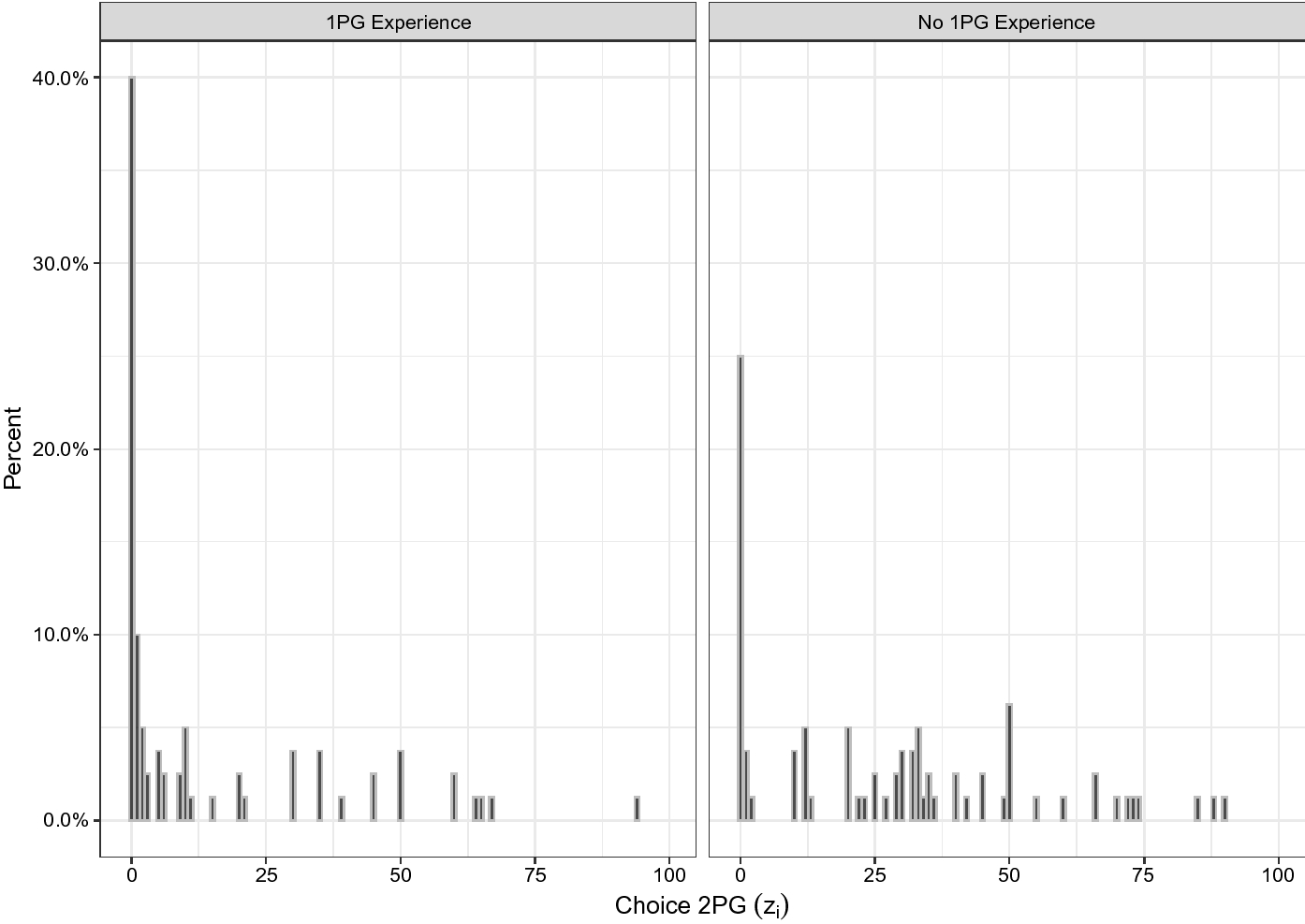
Fig. 2 Distribution of choices in the 2PG with and without 1PG experience
3.2 The two player guessing game
The left panel of Fig. 2 shows the distribution of choices in the 2PG, for subjects who have played the 1PG before. The distribution appears to be quite different from the typical distribution one sees with guessing game “first timers.” The mass of the distribution is close to zero with 50% of subjects playing Nash Equilibrium.Footnote 13 The mean is 13.47 and the median choice is 2. As mentioned in Sect. 2.3.1 we also collected data on 80 subjects who played the 2PG without previously taking part in the 1PG. Choices of these subjects are presented in the right panel of Fig. 2. While a relatively large number of subjects with no prior 1PG experience also play Nash Equilibrium (28.75%), the overall distribution of 2PG choices for those subjects is significantly shifted to the right compared to that of subjects with prior 1PG experience (Kolmogorov Smirnov test, p value
 , see Fig. 14 in "Electronic supplementary material Appendix C" for cumulative density plots). This shift results in a mean and median choice without 1PG experience of 27.8 and 26 respectively.
The difference in behavior between both groups could be the result of two phenomena: introspective learning from having played the 1PG (Weber Reference Weber2003), or a change in the beliefs of subjects that previously played the 1PG given that they are facing a more “experienced” pool of subjects (Agranov et al. Reference Agranov, Potamites, Schotter and Tergiman2012).Footnote 14 In Sect. 3.4.1 we show that shifts of beliefs are relatively small. Therefore, we attribute most of the difference in behavior to introspective learning. So, while most subjects are not able to fully solve the 1PG, there appears to be some learning that carries over to the 2PG.
3.3 Relationship between the 1PG and the 2PG
Figure 3 shows the decisions of subjects in the 2PG on the vertical axis, and their payoffs for the 1PG on the horizontal axis. Subjects who fully solved the 1PG (solid circles) mostly chose zero in the 2PG (24/25, 96%), and picked significantly lower numbers in the 2PG than subjects who did not fully solve the 1PG (Mann–Whitney U Test, p value
 ). In line with this, we also observe that subjects who earn higher payoffs in the 1PG play lower numbers in the 2PG (Spearman
 , p value
 )
)
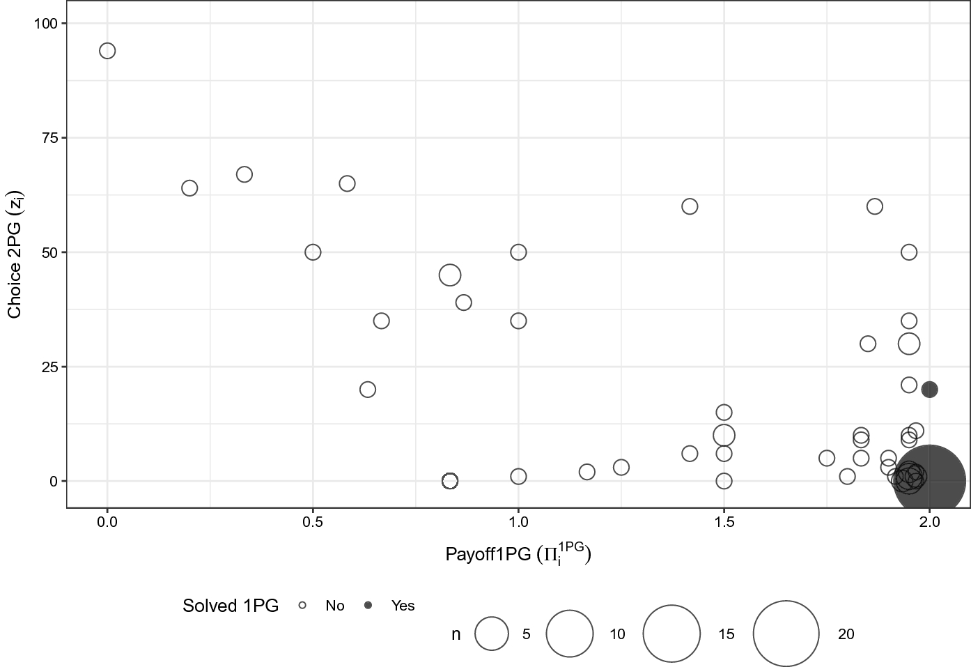
Fig. 3 Distribution of choices in the 2PG (vertical axis) and payoff in the 1PG (horizontal axis)
Result 2
Subjects with a better understanding of the structure of the one-player guessing game play numbers closer to the Nash Equilibrium in the two-player guessing game.
But, is playing numbers near the Nash Equilibrium the best strategy in the 2PG? To answer this question we construct
 . This variable represents the payoff that each subject i would have gotten had she played against the average choice of all other subjects j except herself (i.e.,
 ). Formally
 is defined as:
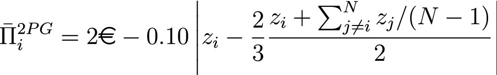
Figure 4 illustrates the relationship of
 with both, the payoffs of the 1PG (
 , left panel) and choice in the 2PG (
 , right panel). Interestingly, subjects who fully solved the 1PG don’t have the highest
 . This is because they play Nash Equilibrium, when payoffs would have been maximized by playing a number close to 9 as can be seen in the right plot. Overall, subjects who fully solved the game did not earn a significantly different payoff compared to subjects who did not fully solve the game (Mann–Whitney U test p value
 ).
).
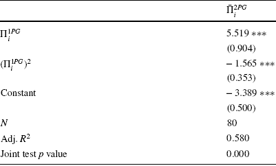
Analyzing our secondary measure of understanding of the structure of the game (
 ) reveals a more nuanced pattern: it appears that there is a non-monotonic relationship between understanding of the structure of the game and expected payoffs in the 2PG (see Fig. 15 in "Electronic supplementary material Appendix C" for a close-up of Fig. 4.). Regressing
 on
on
 and
and
 yields coefficients that are significantly positive and negative respectively. This gives statistical support to the fitted quadratic function in the left panel of Fig. 4, implying that increased understanding leads to increased expected payoffs, but that this relationship reverses for very high levels of understanding.
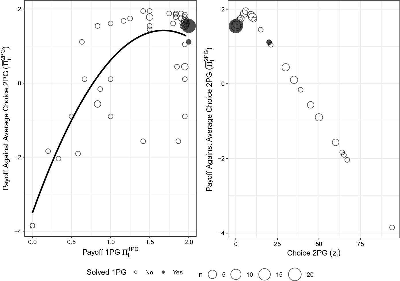
Fig. 4 Relationship of payoff in the 1PG (
 ) and
) and
 (left panel). The line in the left panel is a fitted quadratic function. The right panel shows the relationship of choice in the 2PG (
 ) and
) and
 . In both panels the darker dots indicate subjects who fully solved the 1PG
Table 1 Regression of
 on the payoff in the 1PG (
 ) and its square value

|
|
|
|---|---|
|
|
|
|
(0.904) |
|
|
|
|
|
(0.353) |
|
|
Constant |
|
|
(0.500) |
|
|
|
80 |
|
Adj.
|
0.580 |
|
Joint test p value |
0.000 |


Standard errors in parentheses
*p < 0.05; **p < 0.01; ***p < 0.001
Result 3
The relationship between understanding of the structure of the one-player guessing game and payoffs in the two-player guessing game follows a non-monotonic pattern.
3.4 Subjective beliefs
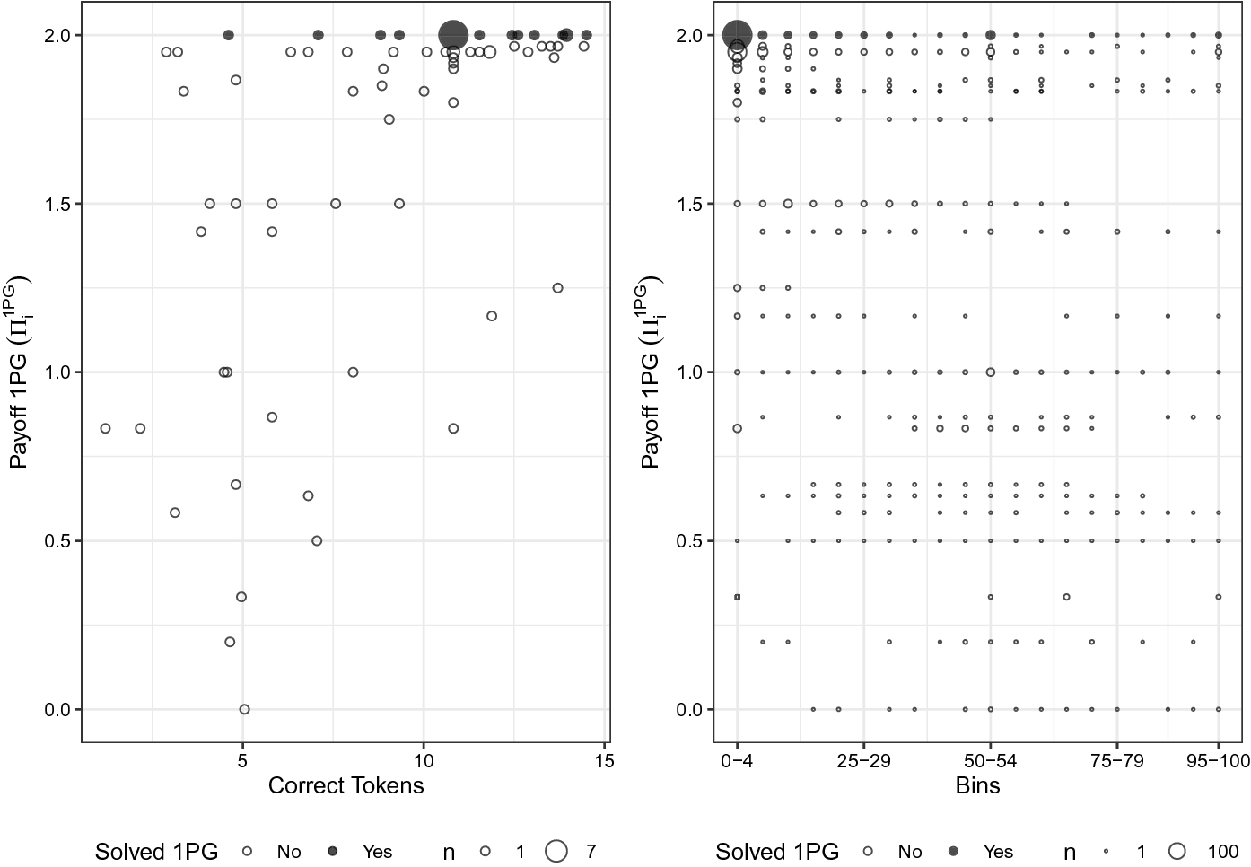
Fig. 5 Relationship between the payoff in the 1PG (
 ) and number of correct tokens deposited in the belief elicitation phase (left panel) and distribution of tokens across bins (right panel). Darker dots refer to subjects who fully solved the 1PG
On the left panel of Fig. 5, we plot the number of tokens subjects have placed correctly in the belief elicitation task against the payoff in the 1PG. Subjects who fully solved the 1PG placed a larger number of tokens correctly (Mann–Whitney U test, p value
 ).Footnote 15 This result is confirmed by the strong correlation that we observe between the 1PG payoff and the number tokens placed correctly (Spearman
 , p value < 0.001). On the right panel of Fig. 5 we plot the distribution of tokens (horizontal axis) against the payoff in the 1PG (vertical axis). While subjects who did not fully solve the 1PG spread out their tokens across most of the strategy space, subjects who fully solved the 1PG expect their counterparts to play numbers closer to the Nash Equilibrium (Mann–Whitney U test, p value
 ). Again, the correlation between the distance of tokens to NE and payoffs in the 1PG confirms this result (Spearman
 with p value
 ) (Table 1).
To test how the accuracy of beliefs relates to the understanding of the structure of the game, we plot the mean of the belief distribution of each subject against their payoff in the 1PG (vertical axis) on the left panel of Fig. 6.Footnote 16 The vertical dotted line marks the mean choice across all subjects in the 2PG (13.63). The right panel of Fig. 6 plots the absolute distance of individual mean beliefs to mean 2PG play against earnings in the 1PG. Two things are clear from the graph: First, the mean beliefs of some subjects differ quite a bit from mean actual play in the 2PG. Second, subjects who fully solved the 1PG have a lower absolute difference of their mean beliefs and mean choice of all subjects in the 2PG (Mann–Whitney U test p value
 ). This result is supported using our secondary measure of understanding (Spearman
 with p value
 ).
).
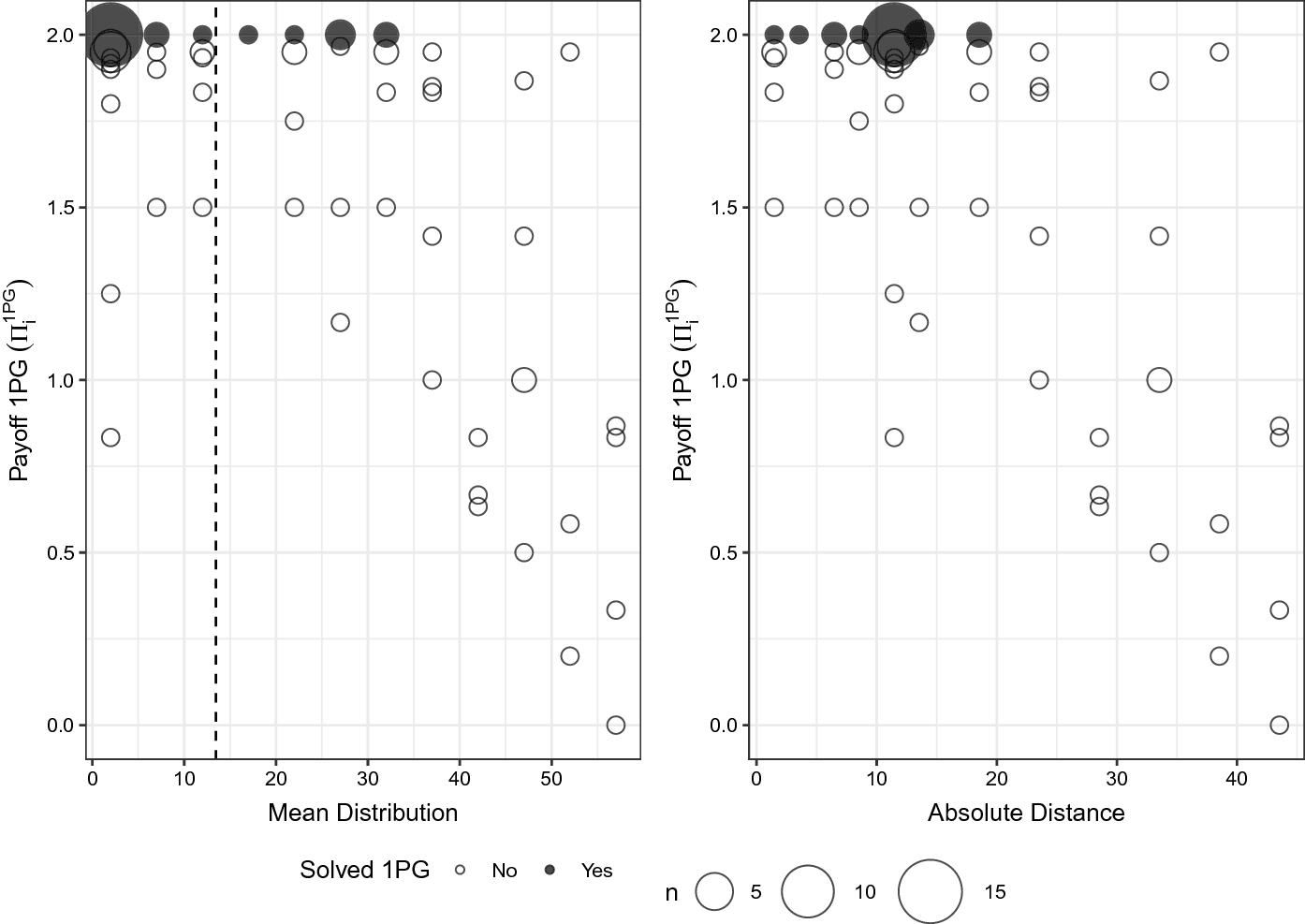
Fig. 6 In the left panel we present the relationship between the payoff in the 1PG (
 ) and the mean value of the distributed tokens (horizontal axis). The vertical dotted line marks the mean of all choices in the 2PG (which is 13.63). The right panel illustrates the relationship between the payoff in the 1PG (
 , vertical axis) and the absolute distance between mean choice of subjects in the 2PG and the mean value of the distributed tokens
Result 4
Subjects with a better understanding of the structure of the one-player guessing game form more accurate beliefs about their counterparts’ choices in the two-player guessing game.
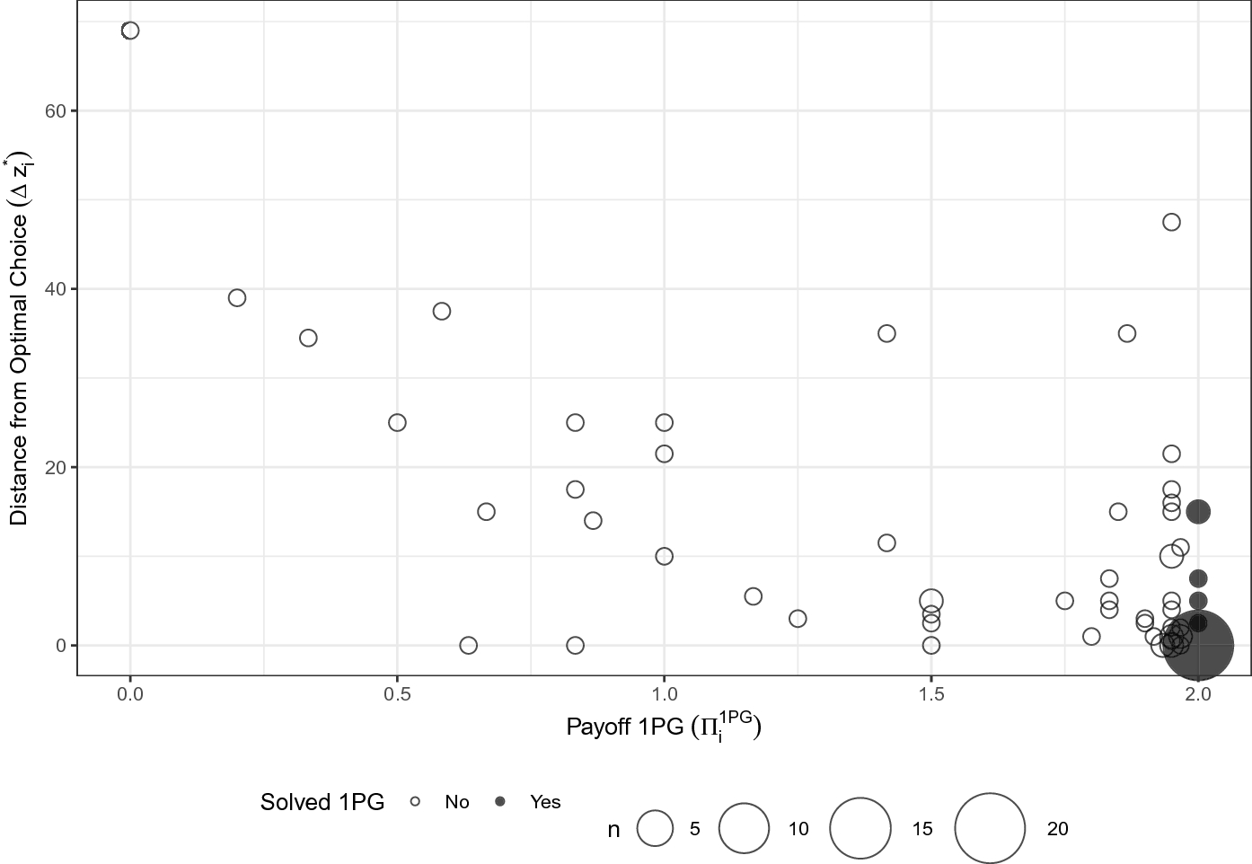
Fig. 7 Difference between actual choice and optimal choice conditional on beliefs (
 ) versus payoff in the 1PG (
 )
)
Additionally, we analyze whether choices in the 2PG are best responses to the stated beliefs (i.e., the token distribution). To do so we compute the choice in the 2PG that would maximize the payoff of a subject conditional on her stated beliefs being correct:
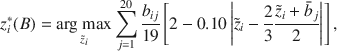
where
 is the choice of subject i that maximizes her payoffs given her beliefs
 ,
,
 is the number of tokens that subject i put in bin j, and
 is the average value of the bin (so for example, for the first bin [0,4],
 , for the second [5,9],
 , etc.).Footnote 17 We then create an individual variable
 which is the absolute difference between actual choice of subject i in the 2PG minus the optimal choice conditional on her stated beliefs. Figure 7 illustrates the relation of
 and the payoffs for the 1PG. It appears that subjects who fully solved the 1PG are better at best responding to their own beliefs and therefore have a lower
 (Mann–Whitney U test p value
 ). This is confirmed by a significantly negative correlation between 1PG payoffs and
 (Spearman
 , p value
 ). These results imply that better understanding of the structure of the guessing game improves the ability to best respond to own beliefs.
Result 5
Subjects with a better understanding of the structure of the one-player guessing game choose numbers closer to the best response of their beliefs in the two-player guessing game.
3.4.1 “What-if” beliefs
As there could be some influence of having played the 1PG on the beliefs in the 2PG, we asked 40 subjects to use 19 tokens to guess the choices of 19 subjects that had played the 2PG “a couple of weeks ago, without having previously played the 1PG”. We will refer to these distributions as “what-if” distributions, as opposed to the elicited distributions in the belief elicitation part of the experiment which we will refer to as “original” distributions.
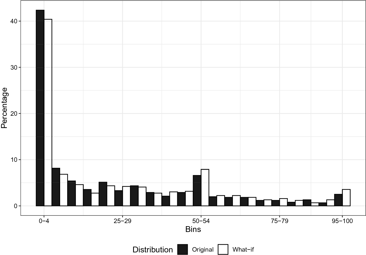
Fig. 8 Distribution of “original” and “what-if” beliefs for the 2PG
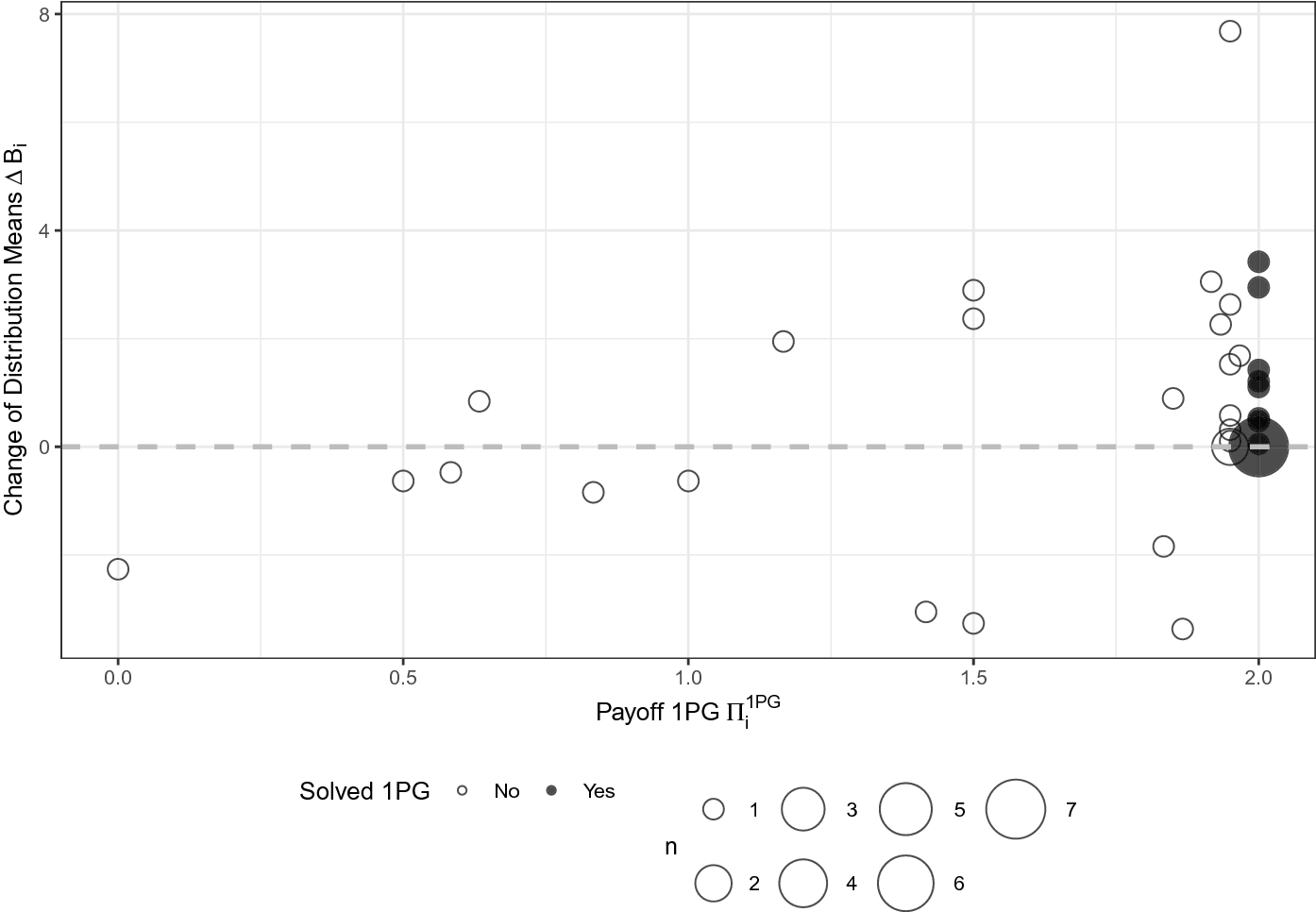
Fig. 9 Payoff in the 1PG on the horizontal axis, and change in the mean between belief distributions (
 ) on the vertical axis. Any value of
 above zero is a change in the mean away from the Nash Equilibrium
We plot the resulting aggregated distributions in Fig. 8. At first glance, the differences between what-if and original distributions appear to be small.Footnote 18 However, when comparing the means and variances of subjects’ individual distributions, we find that both mean and variance are significantly higher in the what-if distributions (Wilcoxon matched-pairs signed-ranks test, p value
 and p value
 for the difference in means and variance respectively). This indicates that subjects adjust their beliefs depending on the population they face.Footnote 19
To get a better understanding of how subjects change their beliefs in the 2PG when faced with different populations, we plot the difference in means between the what-if and original distributions (
 ) against the individual payoff from the 1PG (
 ) in Fig. 9. In this figure, any value above the horizontal dotted line indicates a shift of the what-if distribution, with respect to the original one, away from the NE.
As can be seen in Fig. 9, whenever subjects who fully solved the 1PG adjust their beliefs, they seem to do so in the right direction (i.e., away from the NE). However, we cannot reject the null hypothesis of no differences in the distribution means (
 ) between subjects who fully solved the 1PG and those who did not (Mann–Whitney U Test, p value
 ). Using our secondary measure of understanding, we find a significant correlation between payoffs in the 1PG and
 (Pearson
 , p value
 ), but we cannot reject the hypothesis that this relationship is not monotonic (Spearman
 , p value
 ). Therefore, if we interpret a higher payoff in the 1PG as a better understanding of the structure of the game, then it would appear that a better understanding is associated with better adjustment of beliefs in response to facing an inexperienced population.Footnote 20
Result 6
There is weak evidence suggesting that subjects with a better understanding of the structure of the one-player guessing game are better at adjusting their beliefs in response to facing an inexperienced population in the two-player guessing game.
4 Conclusion
In laboratory experiments, subjects often deviate from equilibrium play. These deviations can be the result of either subjects not understanding the structure of the underlying game or from not forming the correct beliefs about the strategies of their counterparts. One strand of the literature has tried to explain these deviations as errors in belief formation (e.g., Costa-Gomes and Crawford Reference Costa-Gomes and Crawford2006; Ho et al. Reference Ho, Camerer and Weigelt1998). Yet, some recent research shows that subjects might not fully understand the experimental environment.
In this paper we use an individual decision-making task that allows us to uncouple subjects’ understanding of the game from their belief formation, and thus to establish to what extent understanding of the structure of the game contributes to non-equilibrium play in our experiment.
We find that a majority of subjects fail to fully understand the structure of the game. Moreover, subjects who understand the structure of the game play closer to the Nash Equilibrium, are better at best-responding to their own beliefs, and seem to modify their beliefs (correctly) depending on the population they are facing. This result is inconsistent with models of the Level-K type (e.g., Costa-Gomes and Crawford Reference Costa-Gomes and Crawford2006) which assume that agents fully understand the structure of the game and only play out of equilibrium due to flaws in belief formation. Our findings suggest, otherwise, that out of equilibrium play is not only the result of a limited ability to form correct beliefs, but that it also results from the inability of subjects to fully understand the game’s structure.
In light of these results, we believe the 1PG could be a useful “quick and easy” test for researchers interested in, or aiming to control for, understanding of the structure of guessing games. More generally, we believe that the reduction of strategic games into one-player forms could be a useful tool in the analysis of other games too.Footnote 21 Such transformation would allow researchers to study the degree of understanding that subjects have of the structure of the game, and to control for any deviations from Nash equilibrium play independent of errors in belief formation.Footnote 22
Finally, a potential extension of this experiment could be to vary the number of selves subjects play in the 1PG and compare play to standard guessing games populated by the same number of strategic players. On the one hand, increasing the number of selves and strategic players increases the complexity of the game, and may therefore make understanding the structure of the game and belief formation more difficult. On the other hand, increasing the number of selves and strategic players may lead subjects to better understand the unraveling mechanic of the game. We leave it to future extensions of this work to test whether the general findings in this paper would also hold under such conditions.
Acknowledgements
Open Access funding provided by Projekt DEAL. The authors would like to thank David Freeman, Dan Friedman, Yoram Halevy, Frank Heinemann, Rosemarie Nagel, Luba Petersen, Pedro Rey Biel, Christian Seel, and especially Marina Agranov and Yves Breitmoser for their comments. Additionally, the authors acknowledge financial support from the Deutsche Forschungsgemeinschaft (DFG) through CRC 649 “Economic Risk”. The first author thanks the Deutsche Forschungsgemeinschaft (DFG) for funding through the CRC TRR 190 “Rationality and Competition”.


 Πi1PG
Πi1PG Π¯i2PG
 zi
zi Π¯i2PG
 Π¯i2PG
 Πi1PG
Πi1PG (Πi1PG)2
 Πi1PG
Πi1PG
 Πi1PG
Πi1PG Πi1PG
Πi1PG
 Δzi∗
Δzi∗ Πi1PG
Πi1PG

 ΔBi
ΔBi ΔBi
ΔBi


 Open access