


Nomenclature
- c
chord length of blade
- C d
drag coefficient of the aerofoil
- C lα
lift curve slope of blade
- C pk
inflow coupling matrix of wake bending
- C T , C H , C Y , C Q
thrust, backward, sideward forces and torque coefficients of rotor
- h
pylon length
-
 ${{\tilde{L}}} $
gain matrix relating to the skew angle-of-wake
- m s
the blade mass per unit length
- m w
the wing mass per unit length
- m p
the mass of pylon
- M
mass matrix in inflow state equations
- M tip
Mach number of blade tip
- N b
number of blade
- q
dynamic pressure
- q h , p h
longitudinal and lateral tilting angular velocity of pylon
-
$\bar{r}$
dimensionless radius of blade
- x p , y p , z p
translational deformation degrees of freedom of wing tip
- V
forward speed (forward speed V/ΩR)
-
$\overline{{V_{c} }} $
the component of forward speed along pylon
- V
mass flow parameter matrix
- w bi
normal velocity caused by blade motion
- α p
tilt angle-of-pylon
- α x , α y , α z
rotational deformation degrees of freedom of wing tip
-
$\alpha _{j}^{k} $
,
$\beta _{j}^{k} $
state variables of induced inflow
- β, ξ
flapping and lag angle-of-blade
- γ
Lock number of blade
- θ0, θ c , θ s
collective, longitudinal and lateral pitch
- κ′
wake bending influence coefficient
- λ w
vertical induced inflow velocity on the rotor disk
- ϕ
radial expand function
- ψ
azimuth angle
- ω
p
,
$\dot{\omega }_{p} $
tilting angular velocity and acceleration of pylon


1.0 INTRODUCTION
Tiltrotor aircraft has the flight capabilities of a helicopter and turboprop aircraft. The conversion flight between helicopter and turboprop aircraft can be achieved through by tilting the rotor pylon forward. While the pylon is in motion, the tilting rotor is in an unsteady aerodynamic environment and the rotor wake is undergoing bending, which makes the aeroelastic model of tiltrotor aircraft very complicated. Until now, the research on the dynamic stability of the tiltrotor aircraft has been mainly focused on the aeroelastic stability analysis in forward flight( Reference Kim 1 , Reference Kaza 2 ). Active and passive control methods( Reference Singh, Gandhi and Paik 3 , Reference Zhang and Smith 4 ), like wing-flaperon and winglet, aeroelastically tailored blades( Reference Nixon 5 ) and composite wings( Reference Slaby and Smith 6 , Reference Kim, Lim and Shin 7 ) were used to improve the maximum forward flight speed of tiltrotor aircraft. A more accurate rotor inflow model is needed to assess the effects of rotor wake bending while the pylon is undergoing conversion. The Peters–He generalized dynamic inflow theory( Reference He 8 ) takes into account the computational efficiency and accuracy, and has been applied in modelling of aeroelastic stability analysis for helicopters( Reference Venkatesan 9 – Reference Krothapallik, Prasad and Peters 11 ). The author thoroughly studied the dynamic inflow modelling and aeroelastic responses of a rotor undergoing tilting motion( Reference Yue and Xia 12 ), as well as the pylon whirl flutter and the divergent motion of wing of tiltrotor aircraft in forward flight( Reference Li and Xia 13 ). On this basis, combing the rotor wake bending unsteady dynamic inflow model( Reference Yue and Xia 12 ), the unsteady aerodynamic model( Reference Bertin and Smith 14 , Reference Saffman 15 ) and the consideration of structural coupling of rotor/pylon/wing, the nonlinear aeroelastic model of tiltrotor aircraft in conversion flight has been presented in this paper, and the rotor/pylon/wing aeroelastic stability of a tiltrotor aircraft in different flight conditions was calculated and analysed.
2.0 AEROELASTIC MODELLING OF TILTROTOR AIRCRAFT IN CONVERSION FLIGHT
2.1 Dynamic modelling of tiltrotor aircraft
Figure 1 shows the structural dynamic model of a tiltrotor aircraft in conversion flight used in this paper. A rigid-body pylon which can tilt forward and backward about the pivot point is connected to one end of the articulated rotor system, while the other end is mounted at the elastic wing tip (point P). α p is the tilt angle-of-pylon. The tiltrotor aircraft is in helicopter flight mode when the tilt angle is 0°, and in turboprop aircraft flight mode when the angle is 90°. ω p is the tilting angular velocity of pylon. The wing tip degrees of freedom contain three translational degrees of freedom x p , y p , z p and three rotational degrees of freedom α x , α y , α z . h represents the distance between the hub and the pivot point. The first-order modes of global flapping β0, β1c , β1s and global lag ξ0, ξ1c , ξ1s are considered in this paper. The wing of the tiltrotor aircraft is treated as a cantilever beam with concentrated mass installed at end of the beam. The rotor system, wing and pylon constitute a coupled dynamic structural system by structural and motion coupling. The rotor aerodynamic forces and moments are shown in Fig. 1, where T, H, Y and Q are thrust, backward force, sideward force and torque of rotor, respectively (the dimensionless forms are C T , C H , C Y and C Q ). Based on Hamilton’s generalized principle, fully considering the couplings among rotor, pylon and wing of tiltrotor, the equation for a non-conservative system is expressed as
 $${\rm \delta }\Pi {\equals}{\int}_{t_{1} }^{t_{2} } {({\rm \delta }U{\minus}{\rm \delta }T{\minus}{\rm \delta }W)} {\rm d}t{\equals}0$$
where δU, δT and δW are the variations of the elastic strain energy, the kinetic energy and the work done by non-conservative forces, respectively. The contributions to these energy expressions from the blades and wing can be summed as
 $${\rm \delta }U{\equals}\left( {\mathop{\sum}\limits_1^{N_{b} } {{\rm \delta }U_{b} } } \right){\plus}{\rm \delta }U_{W} $$
 $${\rm \delta }T{\equals}\left( {\mathop{\sum}\limits_1^{N_{b} } {{\rm \delta }T_{b} } } \right){\plus}{\rm \delta }T_{W} $$
 $${\rm \delta }W{\equals}\left( {\mathop{\sum}\limits_1^{N_{b} } {{\rm \delta }W_{b} } } \right){\plus}{\rm \delta }W_{W} $$
where the subscript b refers to the blade, W to the wing and N b to the number of blades. The followings are the derivations of the energy terms of wing and rotor.
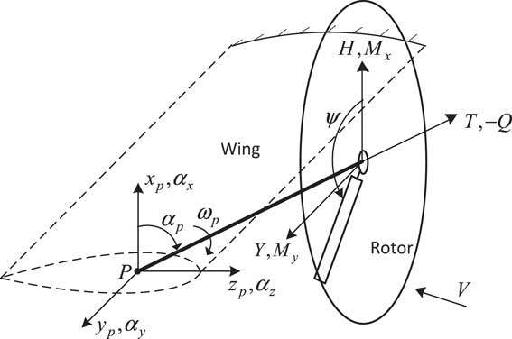
Figure 1 Structural dynamic model of tiltrotor aircraft in conversion flight.
2.2 Dynamic modelling of rotor
According to the positional relationships of each component shown in Fig. 1 and supposing the blade is rigid, the position vector R in inertial co-ordinate system of an arbitrary point on the cross-section at radius r of the ith blade can be expressed as
 $$\eqalignno{ R_{x} {\equals} & r\cos \alpha _{p} \cos \psi {\plus}h\sin \alpha _{p} {\plus}r\beta \sin \alpha _{p} {\plus}r\xi \cos \alpha _{p} \sin \psi {\plus}r\alpha _{x} \sin \alpha _{p} \sin \psi {\plus}h\alpha _{y} \cos \alpha _{p} \cr &{\minus}r\alpha _{y} \sin \alpha _{p} \cos \psi {\minus}r\alpha _{z} \sin \psi {\minus}r\xi \alpha _{x} \sin \alpha _{p} \cos \psi {\plus}r\beta \alpha _{y} \cos \alpha _{p} \cr &{\minus}r\xi \alpha _{y} \sin \alpha _{p} \sin \psi {\plus}r\xi \alpha _{z} \cos \psi {\plus}x_{p} \cr R_{y} {\equals} & r\sin \psi {\minus}r\xi \cos \psi {\minus}h\alpha _{x} {\plus}r\alpha _{z} \cos \alpha _{p} \cos \psi {\minus}r\beta \alpha _{x} {\plus}h\alpha _{z} \sin \alpha _{p} {\plus}r\beta \alpha _{z} \sin \alpha _{p} \cr &{\plus}r\xi \alpha _{z} \cos \alpha _{p} \sin \psi {\plus}y_{p} \cr R_{z} {\equals} & h\cos \alpha _{p} {\minus}r\sin \alpha _{p} \cos \psi {\plus}r\beta \cos \alpha _{p} {\minus}r\xi \sin \alpha _{p} \sin \psi {\plus}r\alpha _{x} \cos \alpha _{p} \sin \psi \cr &{\minus}r\alpha _{y} \cos \alpha _{p} \cos \psi {\minus}h\alpha _{y} \sin \alpha _{p} {\plus}z_{p} {\minus}r\xi \alpha _{x} \cos \alpha _{p} \cos \psi {\minus}r\beta \alpha _{y} \sin \alpha _{p} {\minus}r\xi \alpha _{y} \cos \alpha _{p} \sin \psi $$
where ψ is the azimuth angle, β and ξ are the flapping and the lag angle-of-blade, respectively. The flapping and lag motions of a single blade are transformed into the global flapping and lag motions of rotor by using the Fourier transformation( Reference Johnson 16 ), which are
 $$\beta {\equals}\beta _{0} {\plus}\beta _{{1c}} \cos \,\psi {\plus}\beta _{{1s}} \sin \,\psi $$
 $$\xi {\equals}\xi _{0} {\plus}\xi _{{1c}} \cos \psi {\plus}\xi _{{1s}} \sin \,\psi $$
The velocity of the point is determined by taking the time derivative of the position vector (5) and is given as
 $${\mib{V}} _{b} {\equals}{{\partial {\mib{R}} } \over {\partial t}}$$
The virtual kinetic energy variation of the ith blade is given by
 $${\rm \delta }T_{b} {\equals}{\int}_0^R {m_{s} {\mib{V}} _{b} \cdot {\rm \delta }{\mib{V}} _{b} dr} $$
where m s is the blade mass per unit length, R is the blade radius.
According to the description of rigid body kinematics, the virtual strain energy of the rotor is given by
 $$\delta U_{b} {\equals}K_{\beta } \beta \delta \beta {\plus}K_{\xi } \xi \delta \xi $$
where K β and K ξ flapping and lag stiffness of blade.
2.2 Dynamic modelling of wing and pylon
The structural dynamic model of an elastic wing is established by using finite element discretization method( Reference Nixon 5 ). As shown in Fig. 2, the three velocity components in an inertial co-ordinate system of the velocity V w at a point on the cross section located at x position from the wing root are given by
 $$\eqalignno{ & V_{{wx}} {\equals}\dot{u}_{w} \cr & V_{{wy}} {\equals}\dot{v}_{w} \cr & V_{{wz}} {\equals}\dot{w}_{w} {\plus}y\dot{\phi }_{w} $$
where u w , v w and w w are spanwise, chordwise and vertical translational deformation of wing, respectively, and ϕ w is the torsion of wing. y is the distance between the torsional axis of the wing and the centre of gravity of the section. The variation of virtual kinetic energy of wing is given by
 $${\rm \delta }T_{w} {\equals}{\int}_0^{y_{{tw}} } {m_{w} {\mib{V}} _{{\mib{w}} } \cdot {\rm \delta }{\mib{V}} _{{\mib{w}} } {\rm d}x{\plus}m_{p} {\mib{V}} _{{\mib{w}} } \cdot {\rm \delta }{\mib{V}} _{{\mib{w}} } } $$
where m w is the wing mass per unit length, m p is the rigid pylon mass and y tw is the wing length. The wing is treated as an elastic cantilever beam and modelled by using a finite element method. The variation of virtual strain energy δU w of wing can be found in Ref. 5.
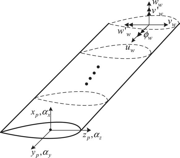
Figure 2 Structural dynamic model of wing.
3.0 UNSTEADY AERODYNAMIC MODEL
The ONERA unsteady aerodynamic model( Reference Bertin and Smith 14 , Reference Saffman 15 ) is used to calculate the unsteady aerodynamic forces in this paper. The aerodynamic forces components of blade aerofoil are shown in Fig. 3.
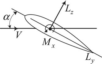
Figure 3 Aerodynamic forces components of blade aerofoil.
In Fig. 3, V is the airflow speed relative to the blade aerofoil, α is the angle-of-attack of the blade aerofoil, L y and L z are the chordwise and normal unsteady aerodynamic forces, respectively. According to the description of ONERA model( Reference Bertin and Smith 14 , Reference Saffman 15 ), the unsteady aerodynamic forces on the aerofoil include the circulation airloads, non-circulation airloads and drag forces, where the circulation airloads can be expressed as
 $$\eqalignno{ & L_{{yc}} {\equals}{\minus}qc{{w_{{b0}} {\minus}\lambda _{{w0}} } \over {v_{{2de}} }}{\mathop{\rm sgn}} (v)\left[ {c_{{l\alpha }} \sin \alpha {\minus}{{c_{{l\alpha }} w_{{b1}} } \over {2v_{{2de}} }}} \right] \cr & L_{{zc}} {\equals}qc{{\left| v \right|} \over {v_{{2de}} }}(c_{{l\alpha }} \sin \alpha ) \cr & M_{{xc}} {\equals}{1 \over 4}cL_{{zc}} {\mathop{\rm sgn}} (v) $$
where w bi (i=0,1,2,3) are normal velocities caused by the blade motions and include the vertical velocities produced by flapping and pitching of the blade, and the tilting of the pylon. λ w0 is the normal velocity component of the unsteady dynamic induced inflow λ w . c is the length of the blade chord, and q is the dynamic pressure. v 2de is the local resultant velocity of aerofoil. For rotor aerodynamic modelling, the reversed flow region cannot be neglected due to large forward flight speed in conversion flight. Therefore, it is necessary to consider the influence of blade chordwise velocity of blade on the magnitude and direction of aerodynamic forces, and terms sgn(v) and |v| in the aerodynamic forces expressions (13) are modified by considering the effects of reversed inflow region. While the rotor is tilting, the inflow produced by forward flight perpendicular to the rotor increases, leading to greater inflow angle of the blade. Therefore, it is necessary to consider the influence of stall on lift coefficient. For different aerofoils, the lift coefficients at different angles of attack can be determined by look-up table method( Reference Johnson 16 ). Since the tiltrotor aircraft can fly at a high speed, it is necessary to consider the stall effect for retreating blade and compressibility for advancing blade. According to Ref. 17, the aerodynamic model is modified by adjusting and substituting the proper lift and drag coefficients under different flight conditions in aerodynamic forces expressions.
The non-circulation aerodynamic forces of the aerofoil come from the airloads produced by the vibration of the aerofoil at the equilibrium position, which are given as
 $$\eqalignno{ & L_{{znc}} {\equals}{1 \over 4}\rho c^{2} \pi (\dot{w}_{{b0}} ) \cr & M_{{xnc}} {\equals}{\minus}{1 \over {64}}\rho c^{3} \pi (\dot{w}_{{b1}} ) $$
where
 $\dot{w}_{{b1}} \,\approx\,{1 \over 2}{\mathop{\rm sgn}} (v)c\ddot{\theta }_{T} .$
The drag forces of the aerofoil can be expressed by
 $$\eqalignno{ & L_{{xd}} {\equals}{1 \over 2}\rho cc_{d} uv_{{3d}} \cr & L_{{yd}} {\equals}{1 \over 2}\rho cc_{d} vv_{{3d}} \cr & L_{{zd}} {\equals}{1 \over 2}\rho cc_{d} wv_{{3d}} $$
where C
d
is the drag coefficients of the aerofoil. v
3d
is the resultant velocity of the aerofoil, and is calculated by
 $v_{{3d}} {\equals}\sqrt {u^{2} {\plus}v^{2} {\plus}w^{2} } $
.
$v_{{3d}} {\equals}\sqrt {u^{2} {\plus}v^{2} {\plus}w^{2} } $
.
The aerodynamic forces on a blade segment can be obtained by adding the circulation, non-circulation and drag aerodynamic airloads in each direction. The non-dimensional aerodynamic forces and moments on rotor shown in Fig. 1 are obtained through the following expressions:
 $$\eqalignno{ & {{M_{F} } \over {C_{{l\alpha }} c}}{\equals}{\int}_0^1 {r{{L_{z} } \over {C_{{l\alpha }} c}}dr} \cr & {{M_{L} } \over {C_{{l\alpha }} c}}{\equals}{\int}_0^1 {r{{L_{y} } \over {C_{{l\alpha }} c}}dr} \cr & {{C_{T} } \over {C_{{l\alpha }} \sigma }}{\equals}{1 \over {N_{b} }}\mathop{\sum}\limits_{i{\equals}1}^{N_{b} } {{\int}_0^1 {r{{L_{z} } \over {C_{{l\alpha }} c}}dr} } \cr & {{C_{Q} } \over {C_{{l\alpha }} \sigma }}{\equals}{\minus}{1 \over {N_{b} }}\mathop{\sum}\limits_{i{\equals}1}^{N_{b} } {{\int}_0^1 {r{{L_{y} } \over {C_{{l\alpha }} c}}dr} } \cr & {{C_{H} } \over {C_{{l\alpha }} \sigma }}{\equals}{1 \over {N_{b} }}\mathop{\sum}\limits_{i{\equals}1}^{N_{b} } {{\int}_0^1 {\left( {{{L_{y} } \over {C_{{l\alpha }} c}}\sin \psi _{i} {\plus}{{L_{x} } \over {C_{{l\alpha }} c}}\cos \psi _{i} } \right)} dr} \cr & {{C_{Y} } \over {C_{{l\alpha }} \sigma }}{\equals}{1 \over {N_{b} }}\mathop{\sum}\limits_{i{\equals}1}^{N_{b} } {{\int}_0^1 {{\minus}{{L_{y} } \over {C_{{l\alpha }} c}}\cos \psi _{i} {\plus}{{L_{x} } \over {C_{{l\alpha }} c}}\sin \psi _{i} } dr} \cr & {{M_{x} } \over {C_{{l\alpha }} c}}{\equals}{1 \over {N_{b} }}\mathop{\sum}\limits_{i{\equals}1}^{N_{b} } {{\int}_0^1 {r{{L_{z} \sin \psi _{i} } \over {C_{{l\alpha }} c}}} dr} \cr & {{M_{y} } \over {C_{{l\alpha }} c}}{\equals}{\minus}{1 \over {N_{b} }}\mathop{\sum}\limits_{i{\equals}1}^{N_{b} } {{\int}_0^1 {r{{L_{z} \cos \psi _{i} } \over {C_{{l\alpha }} c}}} dr} $$
where M F and M L are the flapping and the lag aerodynamic moments, respectively. C T , C H and C Y are thrust, backward force and sideward force coefficients on rotor, respectively. C Q , M x and M y are torque, hub moments in the x- and the y-axis direction due to flapping motion of blades. The aerodynamic forces and moments transmitted to the wing tip can be obtained by the following relationships:
 $$\left[ {\matrix{ {F_{x}^{p} } \hfill \cr {F_{y}^{p} } \hfill \cr {F_{z}^{p} } \hfill \cr {M_{x}^{p} } \hfill \cr {M_{y}^{p} } \hfill \cr {M_{z}^{p} } \hfill \cr } } \right]{\equals}\left[ {\matrix{ {\cos \alpha _{p} } & 0 & {\sin \alpha _{p} } & 0 & 0 & 0 \cr 0 & 1 & 0 & 0 & 0 & 0 \cr {{\minus}\sin \alpha _{p} } & 0 & {\cos \alpha _{p} } & 0 & 0 & 0 \cr 0 & {{\minus}h\cos \alpha _{p} } & 0 & {\cos \alpha _{p} } & 0 & {{\minus}\sin \alpha _{p} } \cr h & 0 & 0 & 0 & 1 & 0 \cr 0 & {{\minus}h\sin \alpha _{p} } & 0 & {\sin \alpha _{p} } & 0 & {\cos \alpha _{p} } \cr } } \right]\left[ {\matrix{ {C_{H} } \hfill \cr {C_{Y} } \hfill \cr {C_{T} } \hfill \cr {M_{x} } \hfill \cr {M_{y} } \hfill \cr {C_{Q} } \hfill \cr } } \right]$$
The virtual work done by external aerodynamic forces of each generalized degrees of freedom is given by
 $$\delta W_{b} {\equals}F_{x}^{p} \delta x_{p} {\plus}F_{y}^{p} \delta y_{p} {\plus}F_{z}^{p} \delta z_{p} {\plus}M_{x}^{p} \delta \alpha _{x} {\plus}M_{y}^{p} \delta \alpha _{y} {\plus}M_{z}^{p} \delta \alpha _{z} {\plus}M_{F} \delta \beta {\plus}M_{L} \delta \xi $$
The aerodynamic forces of wing are obtained by strip theory, and the detailed derivation of virtual work done by aerodynamic forces of wing can be found in Ref. 5.
4.0 WAKE BENDING DYNAMIC INFLOW MODEL OF TILTROTOR
To accurately establish the induced inflow model of a tiltrotor undergoing conversion, the wake bending dynamic inflow model( Reference Yue and Xia 12 ) is used. The model is based on the Peters–He generalized dynamic inflow model( Reference He 8 ) and the modification of rotor wake bending effects. In the wake bending unsteady inflow model, the vertical induced inflow velocity on the rotor disk can be described by a series form of arbitrary order harmonics and radial shape functions
 $${\rm \lambda }_{w} (\overline{r} ,{\rm \psi },t){\equals}\mathop{\sum}\limits_{r{\equals}0}^\infty {\mathop{\sum}\limits_{j{\equals}k{\plus}1,k{\plus}3,...}^\infty {\phi _{j}^{k} } } (\overline{r} )\left[ {{\rm \alpha }_{j}^{k} (t)\cos (k{\rm \psi }){\plus}{\rm \beta }_{j}^{k} (t)\sin (k{\rm \psi })} \right]$$
where λ
w
is the vertical induced inflow velocity on the rotor disk. α and β are the state variables of the induced inflow in the inflow model. k is the harmonic orders of induced inflow, and j is the number of shape functions. t represents time.
 $\bar{r}$
is the non-dimensional radius of the blade. ϕ is the radial expand function which is given as
$\bar{r}$
is the non-dimensional radius of the blade. ϕ is the radial expand function which is given as
 $$\phi _{j}^{k} (\overline{r} ){\equals}\sqrt {(2j{\plus}1)H_{j}^{k} } \mathop{\sum}\limits_{q{\equals}k,k{\plus}2...}^{j{\minus}1} {{{\overline{r} ^{q} ({\minus}1)^{{(q{\minus}k)\,/\,2}} (j{\plus}q)\,!!\,} \over {(q{\minus}k)\,!!\,(q{\plus}k)\,!!\,(j{\minus}q{\minus}1)\,!!\,}}} $$
where
 $H_{j}^{k} {\equals}{{(j{\plus}k{\minus}1)\,!!\,(j{\minus}k{\minus}1)\,!!\,} \over {(j{\plus}k)\,!!\,(j{\minus}k)\,!!\,}}$
.
$H_{j}^{k} {\equals}{{(j{\plus}k{\minus}1)\,!!\,(j{\minus}k{\minus}1)\,!!\,} \over {(j{\plus}k)\,!!\,(j{\minus}k)\,!!\,}}$
.
According to the Peters–He theoretical model, the dimensionless state equations of each cosine and sine state variable are given as,
 $$\eqalignno{ & {\bf{M}} _{c} \left\{ {\alpha _{j}^{k} } \right\}^{{\bullet}} {\plus}{\bf{V}} _{c} {{\tilde{L}}} _{c} ^{{{\minus}1}} \left\{ {\alpha _{j}^{k} } \right\}{\equals}{\bf \tau } _{c} \cr & {\bf{M}} _{s} \left\{ {\beta _{j}^{k} } \right\}^{{\bullet}} {\plus}{\bf{V}} _{s} {{\tilde{L}}} _{s} ^{{{\minus}1}} \left\{ {\beta _{j}^{k} } \right\}{\equals}{\bf \tau } _{s} $$
where M is the mass matrix, V is the mass flow parameter matrix and
 ${{\tilde{L}}} $
is the gain matrix relating to the skew angle-of-wake. τ is the aerodynamic forces’ coefficients on rotor disk. The subscripts c and s represent the cosine and sine terms, the analytical form of the mass matrix M is
${{\tilde{L}}} $
is the gain matrix relating to the skew angle-of-wake. τ is the aerodynamic forces’ coefficients on rotor disk. The subscripts c and s represent the cosine and sine terms, the analytical form of the mass matrix M is
 $$\left[ {\matrix{ \ddots & {} & {} \cr {} & {{{2H_{n}^{m} } \over \pi }} & {} \cr {} & {} & \ddots \cr } } \right]{\equals}\left\{ {\matrix{ {[{\bf{M}} _{{\mib{c}} } ]\matrix{ {} & {} & {m{\equals}0,1,2,...N} \cr } } \cr {[{\bf{M}} _{{\mib{s}} } ]\matrix{ {} & {} & {m{\equals}1,2,3,...N} \cr } } \cr } } \right.$$
The cosine and the sine part of the gain matrix are
 $$[\hskip3pt{{\bf{{\vskip-6pt\tilde}\hskip-2pt{L}}}_{{\mib{c}} } }}]{\equals}\left[ {\matrix{ {} & \vdots & {} \cr \cdots & {{\tilde{L}}}_{{jn}}^{{kmc}} ]} & \cdots \cr {} & \vdots & {} \cr } } \right]$$
and
$$[\hskip3pt{{\bf{{\vskip-6pt\tilde}\hskip-2pt{L}}}_{{\mib{c}} } }}]{\equals}\left[ {\matrix{ {} & \vdots & {} \cr \cdots & {{\tilde{L}}}_{{jn}}^{{kmc}} ]} & \cdots \cr {} & \vdots & {} \cr } } \right]$$
and
 $$[\hskip3pt{{\bf{{\vskip-6pt\tilde}\hskip-2pt{L}}}_{\mib{s}} } }}]{\equals}\left[ {\matrix{ {} & \vdots & {} \cr \cdots & {[{{\tilde{L}}}_{{jn}}^{{kms}} ]} & \cdots \cr {} & \vdots & {} \cr } } \right]$$
respectively, where
$$[\hskip3pt{{\bf{{\vskip-6pt\tilde}\hskip-2pt{L}}}_{\mib{s}} } }}]{\equals}\left[ {\matrix{ {} & \vdots & {} \cr \cdots & {[{{\tilde{L}}}_{{jn}}^{{kms}} ]} & \cdots \cr {} & \vdots & {} \cr } } \right]$$
respectively, where
 $$\eqalignno{ & \left[ {{\tilde{L}}}_{{jn}}^{{0m}} } \right]^{C} {\equals}X^{m} \left[ {\Gamma _{{jn}}^{{0m}} } \right] \cr & \left[ {{\tilde{L}}}_{{jn}}^{{rm}} } \right]^{C} {\equals}[X^{{\left| {m{\minus}k} \right|}} {\plus}({\minus}1)^{l} X^{{\left| {m{\plus}k} \right|}} ]\left[ {\Gamma _{{jn}}^{{km}} } \right] \cr & \left[ {{\tilde{L}}}_{{jn}}^{{km}} } \right]^{S} {\equals}[X^{{\left| {m{\minus}k} \right|}} {\minus}({\minus}1)^{l} X^{{\left| {m{\plus}k} \right|}} ]\left[ {\Gamma _{{jn}}^{{km}} } \right] $$
where
 $l{\equals}\min (k,m)$
,
$l{\equals}\min (k,m)$
,
 $X{\equals}\tan \left| {\chi \,/\,2} \right|$
, and if k+m is even,
$X{\equals}\tan \left| {\chi \,/\,2} \right|$
, and if k+m is even,
 $$\Gamma _{{jn}}^{{km}} {\equals}{{({\minus}1)^{{{{n{\plus}j{\minus}2k} \over 2}}} \cdot 2\sqrt {(2n{\plus}1)(2j{\plus}1)} } \over {\sqrt {H_{n}^{m} H_{j}^{k} } (n{\plus}j)(n{\plus}j{\plus}2)[(n{\minus}j)^{2} {\minus}1]}}$$
; if k+m is odd and j=n±1,
$$\Gamma _{{jn}}^{{km}} {\equals}{{({\minus}1)^{{{{n{\plus}j{\minus}2k} \over 2}}} \cdot 2\sqrt {(2n{\plus}1)(2j{\plus}1)} } \over {\sqrt {H_{n}^{m} H_{j}^{k} } (n{\plus}j)(n{\plus}j{\plus}2)[(n{\minus}j)^{2} {\minus}1]}}$$
; if k+m is odd and j=n±1,
 $\Gamma _{{jn}}^{{km}} {\equals}{{\pi \cdot {\mathop{\rm sgn}} (k{\minus}m)} \over {2\sqrt {H_{n}^{m} H_{j}^{k} (2n{\plus}1)(2j{\plus}1)} }}$
;if k+m is odd and j≠n±1,
$\Gamma _{{jn}}^{{km}} {\equals}{{\pi \cdot {\mathop{\rm sgn}} (k{\minus}m)} \over {2\sqrt {H_{n}^{m} H_{j}^{k} (2n{\plus}1)(2j{\plus}1)} }}$
;if k+m is odd and j≠n±1,
 $\Gamma _{{jn}}^{{rm}} {\equals}0$
.
$\Gamma _{{jn}}^{{rm}} {\equals}0$
.
In above expressions, χ=π/2−α w , where α w is the skew angle-of-wake, defined as
 $$\alpha _{w} {\equals}\tan ^{{{\minus}1}} \left( {{{\lambda _{0} {\plus}\overline{{V_{c} }} } \over {V\cos \alpha _{p} }}} \right)$$
where λ0 is the steady term of the axial inflow.
 $$\overline{{V_{c} }} $$
is the dimensionless velocity components of flight inflow perpendicular to the rotor plane, respectively.
$$\overline{{V_{c} }} $$
is the dimensionless velocity components of flight inflow perpendicular to the rotor plane, respectively.
The mass flow parameter matrix
V
includes
 ${\mib{V}} _{{\mib{c}} } {\equals}\left[ {\matrix{ {V_{m} } & {} \cr {} & {\bar{V}} \cr } } \right]$
and
${\mib{V}} _{{\mib{c}} } {\equals}\left[ {\matrix{ {V_{m} } & {} \cr {} & {\bar{V}} \cr } } \right]$
and
 ${\mib{V}} _{s} {\equals}\left[ {\bar{V}} \right]$
, where V
m
is the parameter associated with the time average inflow, given as
${\mib{V}} _{s} {\equals}\left[ {\bar{V}} \right]$
, where V
m
is the parameter associated with the time average inflow, given as
 $V_{m} {\equals}\sqrt {\mu ^{2} {\plus}(\lambda _{0} {\plus}\overline{V} _{c} )^{2} } $
and
$V_{m} {\equals}\sqrt {\mu ^{2} {\plus}(\lambda _{0} {\plus}\overline{V} _{c} )^{2} } $
and
 $\overline{V} $
is the high order mass flow parameter, defined as
$\overline{V} $
is the high order mass flow parameter, defined as
 $\overline{V} {\equals}[\mu ^{2} {\plus}(\lambda _{0} {\plus}\overline{V} _{c} )(2\lambda _{0} {\plus}\overline{V} _{c} )]\,/\,V_{m} $
.
$\overline{V} {\equals}[\mu ^{2} {\plus}(\lambda _{0} {\plus}\overline{V} _{c} )(2\lambda _{0} {\plus}\overline{V} _{c} )]\,/\,V_{m} $
.
In conversion flight, the incoming airstream does not generally flow perpendicular (through the disk). Also, the pylon is simultaneously tilting, which makes the wake bending occur simultaneously with the tilting of the rotor. According to the vortex tube theory model( Reference Keller 18 ) and considering the rotor wake bending effects, the state equations for each inflow variable are written as
 $$\eqalignno{ & {\bf{M}} _{c} \left\{ {\alpha _{j}^{k} } \right\}^{{\bullet}} {\plus}{\bf{V}} _{c} {{\tilde{L'}}} _{c} ^{{{\minus}1}} \left\{ {\alpha _{j}^{k} } \right\}{\equals}{\bf \tau } _{c} \cr & {\bf{M}} _{s} \left\{ {\beta _{j}^{k} } \right\}^{{\bullet}} {\plus}{\bf{V}} _{s} {{\tilde{L'}}} _{s} ^{{{\minus}1}} \left\{ {\beta _{j}^{k} } \right\}{\equals}{\bf \tau } _{s} $$
where the cosine part
 $${{\tilde{L'}}} _{c} _{{}}^{{}} $$
and sine part
$${{\tilde{L'}}} _{c} _{{}}^{{}} $$
and sine part
 $${{\tilde{L'}}} _{s} _{{}}^{{}} $$
of gain matrix are,
$${{\tilde{L'}}} _{s} _{{}}^{{}} $$
of gain matrix are,
 $$\eqalignno{ & {{\tilde{L'}}} _{c} {\rm {\equals}}{{\tilde{L}}} _{c} {\plus}{\bf{C}} _{{pk}} \kappa _{c} \cr & {{\tilde{L'}}} _{s} {\rm {\equals}}{{\tilde{L}}} _{s} {\plus}{\bf{C}} _{{pk}} \kappa _{s} $$
where C pk is the inflow coupling parameter matrix of wake bending. κ c and κ s are the longitudinal and lateral bending coefficients of wake, which are
 $$\eqalignno{ & \kappa _{c} {\equals}{{q_{h} {\minus}\dot{\beta }_{{1c}} } \over {\lambda _{0} {\plus}\bar{V}_{c} }} \cr & \kappa _{s} {\equals}{{p_{h} {\minus}\dot{\beta }_{{1s}} } \over {\lambda _{0} {\plus}\bar{V}_{c} }} $$
where q
h
and p
h
are the longitudinal and the lateral tilting angular velocity of rotor shaft, respectively.
 $\dot{\beta }_{{1c}} $
and
$\dot{\beta }_{{1c}} $
and
 $\dot{\beta }_{{1s}} $
are the longitudinal and lateral angular velocity of the flapping motion of the rotor disk respectively.
$\dot{\beta }_{{1s}} $
are the longitudinal and lateral angular velocity of the flapping motion of the rotor disk respectively.
The above detailed derivation can be found in Ref. 12.
5.0 ASSEMBLING OF ROTOR/PYLON/WING DYNAMIC MODELS
Substituting the above derived virtual kinetic, strain energy and work expressions into Equation (1) and combining the terms with identical variables, the following expression in matrix form can be obtained
 $${\bf{M}} _{1} {{\ddot{q}}} {\plus}{\bf{C}} _{1} {{\dot{q}}} {\plus}{\bf{K}} _{1} {\bf{q}} {\equals}{\bf{F}} $$
where the column vector q contains the rotor, wing and inflow variables, which is
 $${\mib{q}} {\equals}\{ \beta ,\xi ,x_{p} ,y_{p} ,z_{p} ,\alpha _{x} ,\alpha _{y} ,\alpha _{z} ,u_{w}^{1} ,w_{w}^{1} ,v_{w}^{1} ,\phi _{w}^{1} ,v'_{w}^{1} ,w'_{w}^{1} ,\,\ldots\,,u_{w}^{n} ,w_{w}^{n} ,v_{w}^{n} ,\phi _{w}^{n} ,v'_{w}^{n} ,w'_{w}^{n} ,\alpha _{j}^{k} ,\beta _{j}^{k} \} ^{T} $$
As shown in Fig. 2, the rotor is coupled with the pylon/wing system by six degrees of freedom between the hub and wing tip. Without considering of the wing sweep angle, the transformation relationship between the wing tip degrees of freedom and elastic beam degrees of freedom of wing is given by
 $$\left[ {\matrix{ {x_{p} } \cr {y_{p} } \cr {z_{p} } \cr {\alpha _{x} } \cr {\alpha _{y} } \cr {\alpha _{z} } \cr } } \right]{\equals}\left[ {\matrix{ {\cos \alpha _{p} } & 0 & {{\minus}\sin \alpha _{p} } & 0 & 0 & 0 \cr 0 & 1 & 0 & 0 & 0 & 0 \cr {\sin \alpha _{p} } & 0 & {\cos \alpha _{p} } & 0 & 0 & 0 \cr 0 & 0 & 0 & {\cos \alpha _{p} } & 0 & {{\minus}\sin \alpha _{p} } \cr 0 & 0 & 0 & 0 & 1 & 0 \cr 0 & 0 & 0 & {\sin \alpha _{p} } & 0 & {\cos \alpha _{p} } \cr } } \right]\left[ {\matrix{ 0 & 1 & 0 & h & 0 & 0 \cr 1 & 0 & 0 & 0 & {{\minus}h} & 0 \cr 0 & 0 & 1 & 0 & 0 & 0 \cr 0 & 0 & 0 & 0 & 1 & 0 \cr 0 & 0 & 0 & 1 & 0 & 0 \cr 0 & 0 & 0 & 0 & 0 & 1 \cr } } \right]\left[ {\matrix{ {u_{{tip}} } \cr {w_{{tip}} } \cr {v_{{tip}} } \cr {\phi _{{tip}} } \cr {v'_{{tip}} } \cr {w'_{{tip}} } \cr } } \right]$$
The differential equations of tiltrotor aircraft in conversion flight can be obtained by substituting and assembling Equation (29), the Fourier transformation expressions (6) and (7) into Equation (28), and combing with the inflow state equations (25)
 $${{M\ddot{\bf{x}}} {\plus}{\bf{C}} (\psi ){{\dot{\bf{x}}}} {\plus}{\bf{K}} (\psi ){\bf{x}} {\equals}{\bf{F}} $$
where M, C and K are the mass, damping and stiffness matrices of the system, respectively, and the damping and stiffness matrices are varied with the blade azimuth angle. x is the column vector consisting of the system variables. In this paper, taking articulated rotor with three blades, discretizing the elastic wing into six finite element nodes, adopting two harmonics of induced flow (r=2) and three shape functions for each harmonic (j=3), the vector x is defined as
 $$\eqalignno{ & {\mib{x}} {\equals}\{ {\mib{x}} _{{\mib{r}} } ,{\mib{x}} _{{\mib{w}} } ,{\mib{x}} _{\lambda } \} ^{T} {\equals}\{ \beta _{0} ,\beta _{{1c}} ,\beta _{{1s}} ,\xi _{0} ,\xi _{{1c}} ,\xi _{{1s}} ,u_{w}^{1} ,v_{w}^{1} ,\phi _{w}^{1} ,v'_{w}^{^1} ,w'_{w}^{^1} ,\,\ldots\,,\cr &u_{w}^{6} ,v_{w}^{6} ,\phi _{w}^{6} ,v'_{w}^{6} ,w'_{w}^{6} ,\alpha _{1}^{0} ,\alpha _{3}^{0} ,\alpha _{5}^{0} , \quad \alpha _{2}^{1} ,\alpha _{4}^{1} ,\alpha _{6}^{1} ,\alpha _{3}^{2} ,\alpha _{5}^{2} ,\alpha _{7}^{2} ,\beta _{2}^{1} ,\beta _{4}^{1} ,\beta _{6}^{1} ,\beta _{3}^{2} ,\beta _{5}^{2} ,\beta _{7}^{2} \} ^{T} $$
The size of coefficients matrices in Equation (30) is 51×51. The right side F of Equation (30) includes the external aerodynamic force terms, non-linear terms and constant terms independent of variables.
6.0 Solution for aeroelastic stability
6.1 Trim calculation
The trim calculation of the tiltrotor aircraft in conversion flight was carried out by the wind tunnel trim method( Reference Johnson 16 ). First, the flight condition is determined by the given tilt angle of the pylon and the forward speed. The trim control inputs are determined by calculating the response of each pitch input with time at specified lift coefficient of rotor( Reference Peters, Kim and Chen 19 ). The coefficient terms related to trim control inputs θ0, θ c and θ s are moved to the left side in Equation (30), and the trim control equations are introduced as
 $$\left[ {\matrix{ {\tau _{0} } & 0 & 0 \cr 0 & {\tau _{1} } & 0 \cr 0 & 0 & {\tau _{1} } \cr } } \right]\left( {\matrix{ {\theta _{0} } \cr {\theta _{s} } \cr {\theta _{c} } \cr } } \right)^{{ \cdot \cdot }} {\plus}\left( {\matrix{ {\theta _{0} } \cr {\theta _{s} } \cr {\theta _{c} } \cr } } \right)^{ \cdot } {\equals}\left[ {\matrix{ {K_{0} } & 0 & 0 \cr 0 & {K_{1} } & 0 \cr 0 & 0 & {K_{1} } \cr } } \right]\left[ {\matrix{ {{6 \over {C_{{l\alpha }} }}} & 0 & 0 \cr 0 & {{{8\left( {\upsilon _{\beta }^{2} {\minus}1} \right)} \over \gamma }} & {{\minus}1} \cr 0 & 1 & {{{8(\upsilon _{\beta }^{2} {\minus}1)} \over \gamma }} \cr } } \right]\left[ {\matrix{ {\bar{C}_{T} {\minus}C_{T} } \cr {\bar{\beta }_{s} {\minus}\beta _{s} } \cr {\bar{\beta }_{c} {\minus}\beta _{c} } \cr } } \right]$$
where τ0, τ1, K
0 and K
1 are parameters controlling the convergence speed of the trim calculation.
 $\overline{{C_{T} }} $
,
$\overline{{C_{T} }} $
,
 $\overline{{\beta _{c} }} $
and
$\overline{{\beta _{c} }} $
and
 $\overline{{\beta _{s} }} $
are objective values of trim parameters. The trim control dynamic equation is obtained by combing Equations (30) and (31)
$\overline{{\beta _{s} }} $
are objective values of trim parameters. The trim control dynamic equation is obtained by combing Equations (30) and (31)
 $${\bf{M}} _{c} \ddot{x}_{c} {\plus}{\bf{C}} _{c} \dot{x}_{c} {\plus}{\bf{K}} _{c} x_{c} {\equals}{\bf{F}} _{c} $$
where x c ={x r , x w , x λ , x θ }T and x θ ={θ0, θ c , θ s }T, in which θ0 is the collective pitch, θ c and θ s are the longitudinal and the lateral cyclic pitch, respectively. The trim control inputs are determined by calculating the responses of Equation (32) at zero initial conditions, and the responses of each variable are obtained by calculating the response of Equation (30) with the trimmed inputs.
6.2 Linearization of nonlinear equations
The nonlinear terms at the right side of Equation (30) need to be linearized about a trim point to facilitate the solution procedure for stability analysis. Unsteady aerodynamic forces produce oscillations about the equilibrium position of aerofoil in conversion flight. The small perturbation assumption method is used here, and each variable can be treated as small perturbation about the trimmed values, which are written as
 $$\eqalignno{ & {\bf{x}} _{R} {\equals}{\bf{x}} _{{R0}} {\plus}\Delta {\bf{x}} _{R} \cr & {\bf{x}} _{w} {\equals}{\bf{x}} _{{w0}} {\plus}\Delta {\bf{x}} _{w} \cr & {\bf{x}} _{\lambda } {\equals}{\bf{x}} _{{\lambda 0}} {\plus}\Delta {\bf{x}} _{\lambda } $$
The dynamic equations for aeroelastic stability analysis of tiltrotor can be obtained by substituting the expression (33) into Equation (30), and eliminating the higher order perturbation terms, which are
 $${\bf{M}} \Delta {{\ddot{\bf{x}}}} {\plus}{\bf{C}} _{0} (\psi )\Delta {{\dot{\bf{x}}}} {\plus}{\bf{K}} _{0} (\psi )\Delta {\bf{x}} {\equals}0$$
where C 0 and K 0 are linearized damping and stiffness matrices.
6.3 Stability solution
In conversion flight, the damping and stiffness matrices in Equation (34) vary periodically with blade azimuth angle, and the matrices satisfy the relations
 $$\eqalignno{ & {\bf{C}} _{0} (\psi _{0} ){\equals}{\bf{C}} _{0} (\psi _{0} {\plus}2\pi ) \cr & {\bf{K}} _{0} (\psi _{0} ){\equals}{\bf{K}} _{0} (\psi _{0} {\plus}2\pi ) $$
The stability analysis of dynamic equations with periodic coefficients is carried out by using Floquet theory, and Equation (34) is transformed into a first-order differential equation in the state space, which is
 $$\dot{Y}{\equals}{\bf{A}} (\psi )Y$$
where
 $Y{\equals}\{ \Delta x_{R} ,\Delta \dot{x}_{R} ,\Delta x_{W} ,\Delta \dot{x}_{W} ,\Delta x_{\lambda } \} $
, and A(ψ) is the state matrix consisting of periodic coefficients. According to Floquet theory, the transition matrix [Φ(t, t
0)] is obtained by using the fourth-order Runge–Kutta method to calculate the total response of Equation (36) over one time period. The eigenvalues and eigenvectors of [Φ(t, t
0)] at the end point of one time period (t=t
0+2π) are also obtained. The negative real parts of the eigenvalues are the modal damping, and the system is unstable if any modal damping is less than 0.
$Y{\equals}\{ \Delta x_{R} ,\Delta \dot{x}_{R} ,\Delta x_{W} ,\Delta \dot{x}_{W} ,\Delta x_{\lambda } \} $
, and A(ψ) is the state matrix consisting of periodic coefficients. According to Floquet theory, the transition matrix [Φ(t, t
0)] is obtained by using the fourth-order Runge–Kutta method to calculate the total response of Equation (36) over one time period. The eigenvalues and eigenvectors of [Φ(t, t
0)] at the end point of one time period (t=t
0+2π) are also obtained. The negative real parts of the eigenvalues are the modal damping, and the system is unstable if any modal damping is less than 0.
7.0 STABILITY ANALYSIS OF TILTROTOR AIRCRAFT
The test model parameters of a tiltrotor aircraft( Reference Johnson 17 ) are used as the baseline study in this paper, and the main parameters of rotor and wing are listed in Table 1.
Table 1 Main parameters of rotor and wing
7.1 Trim analysis of tiltrotor aircraft
The variation of the tilt angle-of-pylon with time is shown in Fig. 4. In the first 2 s, the rotor is trimmed in helicopter flight mode, and no wake bending occurs since the pylon does not tilt. The pylon tilts from the second seconds to the 7th seconds at a constant angular velocity of 18° per second. The tilt angle of the pylon becomes 90° at the end of the seventh second, with the tiltrotor aircraft entering into aircraft flight mode and achieving an axial flow condition. According to the parameters listed in Table 1, the transient responses of collective θ0 and cyclic pitch θ c , θ s for rotor trim with time at different forward speeds are calculated when the pylon tilts continuously. The calculated results using wake bending unsteady dynamic inflow are compared with a uniform inflow assumption, as shown in Figs 5–10. In particular, Figs 5–7 show the variation of trimmed pitch values with time for a forward speed 0.3 and Figs 8–10 show a forward speed of 0.5. Together, these figures show that while the pylon tilts forward and the tiltrotor aircraft converts from the helicopter flight mode to aircraft flight mode, the velocity component of forward velocity along the rotor shaft direction increases, leading to an increase in the inflow angle of the blade section. Hence, the collective pitch is increased to manage the thrust. During the forward tilting of the pylon, the bending inflow distribution in conversion flight becomes a symmetric distribution in aircraft flight, and the cyclic pitch eventually becomes 0 in aircraft flight mode. The difference in trimmed control inputs between the assumptions of allowing wake bending unsteady dynamic inflow compared with the uniform inflow assumption is mainly seen in the lateral cyclic pitch θ c , indicating that the bending wake unsteady dynamic inflow is mainly trimmed by lateral cyclic pitch while the pylon is tilting. As the pylon tilts forward and the forward speed increases, the forward velocity component along the rotor shaft direction increases, becoming much larger than the unsteady induced inflow in magnitude, and the influence of wake bending unsteady dynamic inflow on the control inputs gradually reduces.
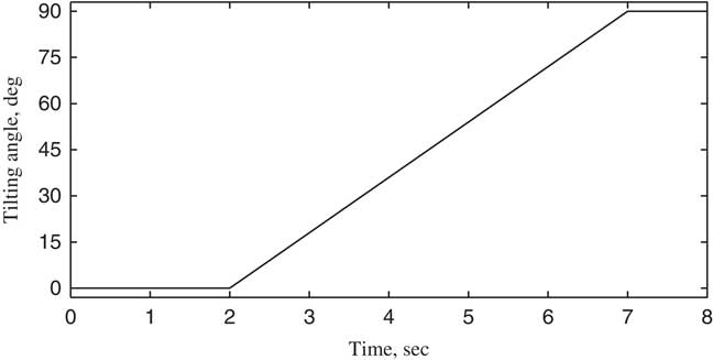
Figure 4 Tilt angle-of-pylon α p changing with time.
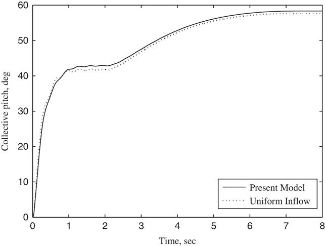
Figure 5 Collective pitch θ 0 changing with time (V/ΩR=0.3).
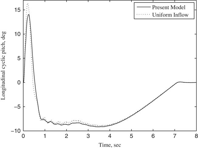
Figure 6 Longitudinal cyclic pitch θ s changing with time (V/ΩR=0.3).
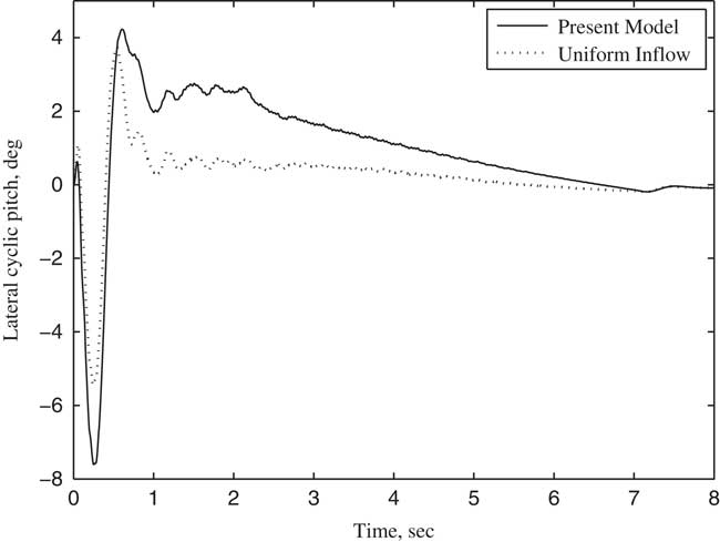
Figure 7 Lateral cyclic pitch θ c changing with time (V/ΩR=0.3).
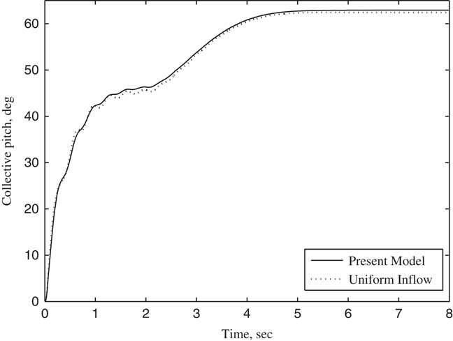
Figure 8 Collective pitch θ 0 changing with time (V/ΩR=0.5).
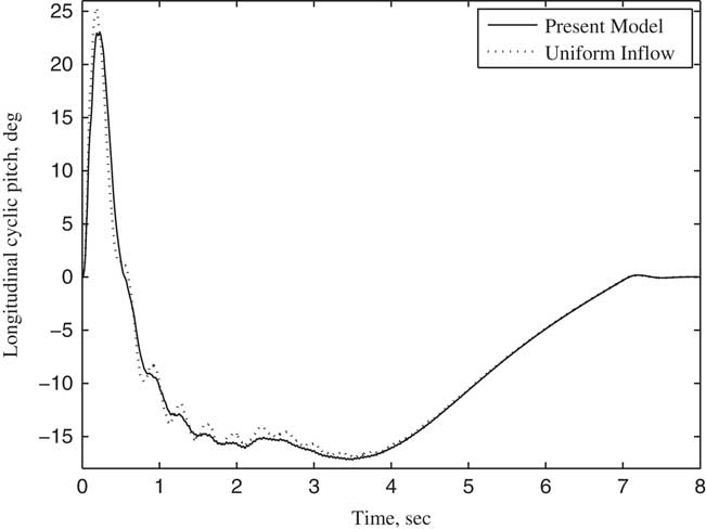
Figure 9 Longitudinal cyclic pitch θ s changing with time (V/ΩR=0.5).
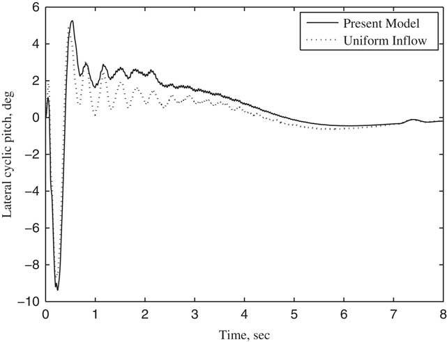
Figure 10 Lateral cyclic pitch θ c changing with time (V/ΩR=0.5).
7.2 Stability analysis of tiltrotor aircraft in conversion flight
The non-linear dynamic equations were linearized on the basis of the steady response of each variable by using trimmed control inputs, and the stability analysis of tiltrotor aircraft in conversion flight was conducted in this paper. According to Ref. 20, the tiltrotor aircraft usually enters into the conversion flight at the forward speed between 0.3 and 0.5. Therefore, the stability analysis is investigated by calculating the variations of modal damping with the tilt angle-of-pylon at the forward speed of 0.3 and 0.5, respectively, which are shown in Figs 11–16. The terms p, q 1 and q 2 represent, respectively, the first order torsional, vertical bending and chordwise bending modes of the wing. It can be seen from Figs 11–14, when the pylon tilts forward, more collective pitch is needed for trimming, which aggravates the structural coupling between flapping and lag of blade, leading a decrease in the frequencies of lag modes ξ s , ξ c and a slight increase in the frequencies of flapping modes β0, β c , β s , and the changing in frequencies of flapping and lag modes with tilt angle become more obvious as the forward speed increases. The unsteady wake bending dynamic inflow produces a slight influence on the frequencies of the blade flapping modes, but has little influence on the frequencies of lag modes and wing modes. As shown in Figs 12–15, the damping of flapping modes reduces with the consideration of the wake bending unsteady dynamic inflow, indicating that the unsteady inflow has significant influence on rotor lift. It can be seen in Figs 13–16, that while the pylon is in motion, tilting to horizontal and forward, which makes damping of the wing first vertical bending mode q 1 less and while increasing the damping of the wing first chordwise bending mode q 2 with the forward tilting of pylon. When the frequency of ξ c and q 2 approaches, abrupt changes of corresponding modal damping occur. When the forward speed is 0.5, the damping of the wing first chordwise bending mode q 2 is negative as the pylon tilts about 23°, making the wing first chordwise bending mode q 2 unstable. Since the aerodynamic forces of rotor and wing increase with the increase of forward speed, the coupling between the modes makes the instability more prone to occur at higher forward speed for the given conditions.
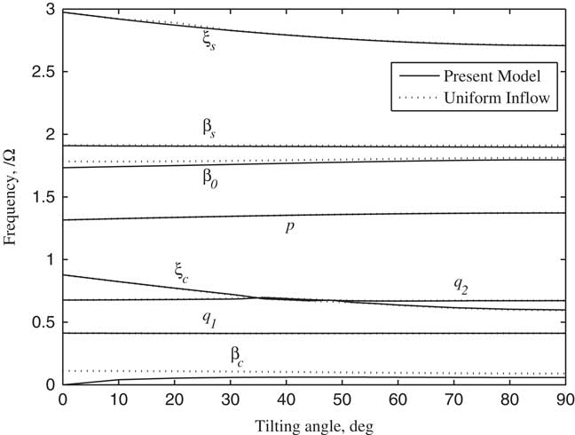
Figure 11 Frequencies of rotor and wing modes changing with tilt angle-of-pylon (V/ΩR=0.3).
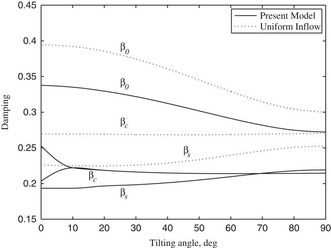
Figure 12 Damping of flapping modes changing with tilt angle-of-pylon (V/ΩR=0.3).
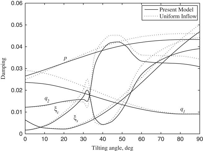
Figure 13 Damping of lag and wing modes changing with tilt angle-of-pylon (V/ΩR=0.3).
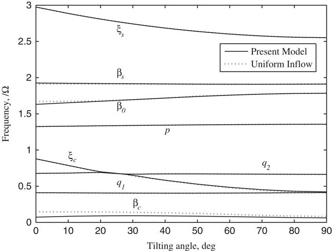
Figure 14 Frequencies of rotor and wing modes changing with tilt angle-of-pylon (V/ΩR=0.5).
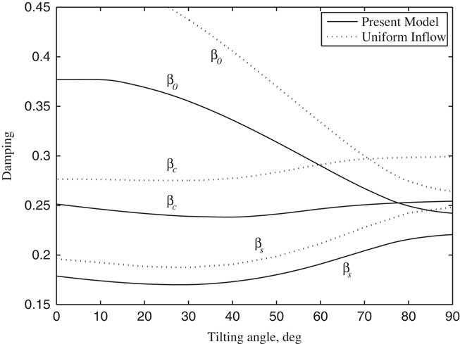
Figure 15 Damping of flapping modes changing with tilt angle-of-pylon (V/ΩR=0.5).
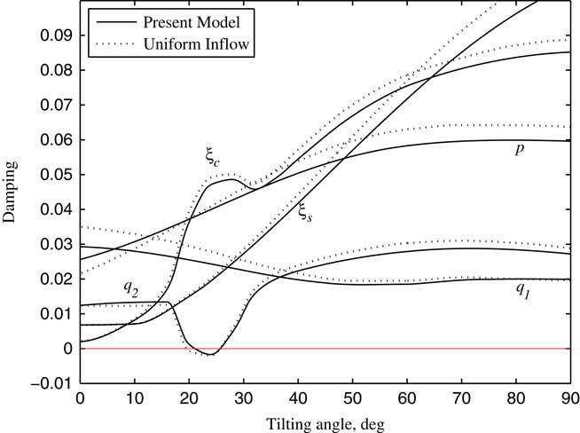
Figure 16 Damping of lag modes and wing bending modes changing with tilt angle-of-pylon (V/ΩR=0.5).
According to the above analysis, the system instability is mainly due to the coupling between the lag modes of the rotor and the bending/torsional modes of the wing. To analyse the aeroelasticity of tiltrotor aircraft at different tilt angles, the variations of each cyclic lag and wing modal frequency and damping with forward flight speed at different tilt angle-of-pylon are calculated and plotted in Figs 17–24, in which the calculations without wake bending dynamic inflow assumption are also shown for comparison. From Figs 17–22, the figures show the helicopter flight mode and the conversion flight mode in which the shown maximum forward speeds are V/ΩR=0.6. Figures 23 and 24 show the turboprop aircraft flight mode in which the shown maximum forward speeds are V/ΩR=1.5. It can be seen from Fig. 17 that the tilt angle-of-pylon is 0° for helicopter flight, where the pylon does not tilt and no wake bending effect on rotor occurs. The frequency of β c mode gradually increases at a high forward speed due to the rotor pitch/flap coupling coefficient. The aerodynamic forces on the rotor plane increase as the forward speed increases, in which the thrust perpendicular to the rotor plane increases, leading to an increase on the damping of the wing first vertical bending mode q 1, and aerodynamic moments produced by the forces parallel to the rotor plane increase, leading to a decrease on the damping of the wing first torsional mode p. According to the above analysis, the wake bending dynamic inflow reduces the aerodynamic forces on the rotor plane, which causes a decrease in the damping of the wing first vertical bending mode q 1 and an increase in the damping of the wing first torsional mode p.
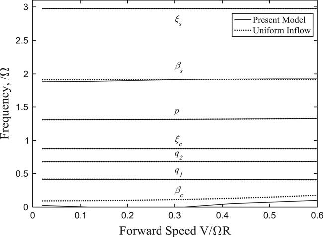
Figure 17 Frequencies of rotor and wing modes changing with forward speed (α p =0°).
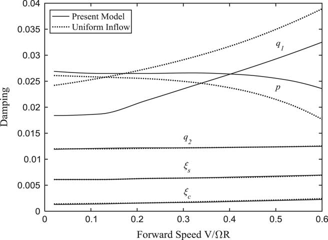
Figure 18 Damping of lag and wing modes changing with forward speed (α p =0°).
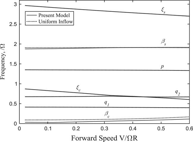
Figure 19 Frequencies of rotor and wing modes changing with forward speed (α p =30°).
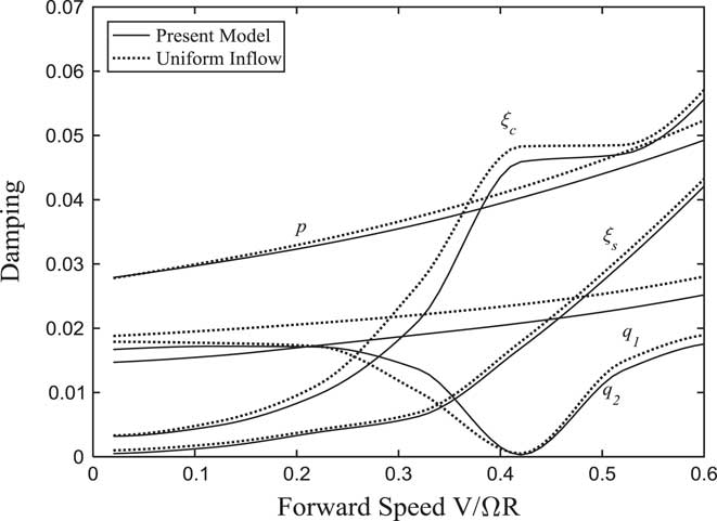
Figure 20 Damping of lag and wing modes changing with forward speed (α p =30°).

Figure 21 Frequencies of lag and wing modes changing with forward speed (α p =60°).
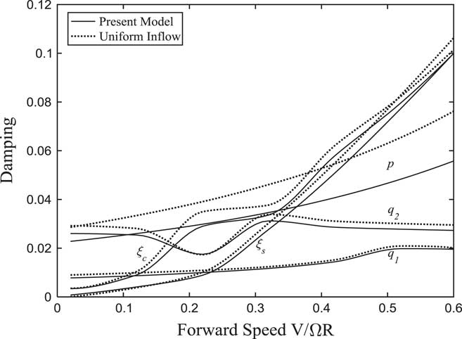
Figure 22 Damping of lag and wing modes changing with forward speed (α p =60°).
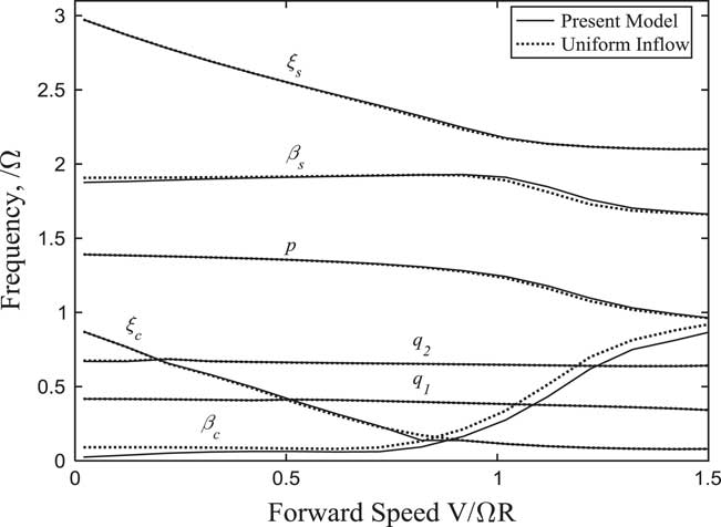
Figure 23 Frequencies of rotor and wing modes changing with forward speed (α p =90°).
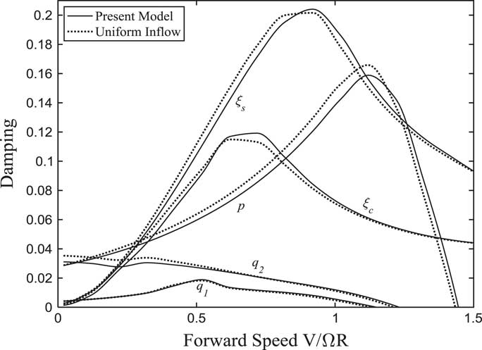
Figure 24 Damping of lag and wing modes changing with forward speed (α p =90°).
The variations of each modal frequency and damping with forward flight speed in conversion flight are plotted in Figs 19–22. It can be seen that the forward tilting motion of pylon causes the frequencies of lag modes to decrease as the forward velocity increases. When the frequency of ξ c is close to the frequency of the wing first vertical bending mode q 1 and chordwise bending mode q 2, a sudden change in damping for corresponding modes and obvious couplings between the modes appear. This can be seen in Fig. 20, when the tilt angle-of-pylon is 30° and the forward speed is 0.41, the damping of the wing first chordwise bending mode q 2 is very close to 0. Since the component of forward velocity along the rotor shaft direction is much greater than unsteady induced inflow in high-speed flight, the influence of wake bending dynamic inflow on the system stability becomes insignificant.
When the tilt angle-of-pylon is 90°, the tiltrotor aircraft is in turboprop aircraft flight mode. In this case, the rotor is in axial flight and no wake bending occurs. The variations of each modal frequency and damping with forward flight speed are plotted in Figs 23 and 24. It can be seen from Fig. 24 that the component of forward velocity along the rotor shaft direction is much greater than wake bending unsteady dynamic inflow, thus the influence of dynamic inflow is not obvious. The damping of the wing first vertical bending mode q 1 is less than 0 and the system is unstable at the forward speed 1.12. The instability form is the divergent vertical motion of wing tip, which is consistent with stability analysis in forward flight( Reference Nixon 5 ).
8.0 CONCLUSION
In this paper, an aeroelastic stability analysis model for a tiltrotor aircraft in conversion flight has been proposed by using a rotor wake bending model, an unsteady dynamic inflow model, an unsteady aerodynamic model, and the structural coupling of rotor/pylon/wing. The results indicate that (1) compared with the uniform inflow model, the unsteady wake bending dynamic inflow is mainly trimmed by lateral cyclic pitch θ c ; (2) the unsteady wake bending dynamic inflow has significant influence on rotor flapping modes, decreasing the damping of each flapping mode, and the influence of unsteady inflow on lag and wing modes is insignificant; (3) in conversion flight, when the pylon tilts at a high forward speed, the instability occurs in chordwise bending mode of wing; (4) in turboprop aircraft flight mode, the unsteady wake bending dynamic inflow has little influence on the stability of tiltrotor aircraft in forward flight.


