


1. Introduction
Emulsions are encountered in a variety of environments, such as multiphase flow through fibrous materials, packed beds with complex pellet shapes and tortuous subsurface settings. Fields ranging from separations processes to oil recovery to microfluidics stand to profit from understanding of Stokes-flow droplet behaviour near complex surfaces. Efforts toward high-resolution microscale numerical models of non-wetting emulsions in complex environments have been stymied, chiefly due to the extremely close approach of fluid–fluid interfaces to solid surfaces. The intervening lubrication layer critically influences the interfacial dynamics, making it difficult to use a simplifying theory for these regions, while also presenting formidable challenges for numerical methods. To overcome some of these limitations, we introduce an extension to the boundary-integral method that leverages both adaptive meshing and high-order singularity subtraction to allow simulation of tight-squeezing drop motion between arbitrarily shaped smooth solid surfaces.
Although a common model for porous media is an ensemble of spherical particles packed in space, several interesting classes of material fall outside this description, such as packed beds of pellets or extrudates, fibrous material or experimental set-ups such as planar constrictions. Probing detailed flow behaviour in such cases is difficult, but there is a growing focus on pore-scale resolution (Blunt et al. Reference Blunt, Bijeljic, Dong, Gharbi, Iglauer, Mostaghimi, Paluszny and Pentland2013). Experimental velocimetry methods, such as magnetic resonance or X-ray tomography (Al-Abduwani et al. Reference Al-Abduwani, Farajzadeh, van den Broek, Currie and Zitha2005; Huang et al. Reference Huang, Mikolajczyk, Küstermann, Wilhelm, Odenbach and Dreher2017), for visualizing and quantifying confined flows are continually improving, strengthening the relationship with computational studies that can provide direct comparisons. For example, Zarikos et al. (Reference Zarikos, Terzis, Hassanizadeh and Weigand2018) used particle-tracking velocimetry to track the interface as well as internal circulation of non-wetting drops as they are trapped and remobilized within porous media. Krummel et al. (Reference Krummel, Datta, Münster and Weitz2013) and Oughanem et al. (Reference Oughanem, Youssef, Bauer, Peysson, Maire and Vizika2015) investigated the recovery of trapped oil, based on capillary number and oil ganglia size distribution, and they were able to resolve individual drops using confocal microscopy and high-resolution micro-computed tomography, respectively. Using similar techniques, Pak et al. (Reference Pak, Butler, Geiger, van Dijke and Sorbie2015) identified a new single-pore mechanism of drop fragmentation. Herring et al. (Reference Herring, Harper, Andersson, Sheppard, Bay and Wildenschild2013) demonstrate the dramatic effect that pore geometry has on the shape and connectivity of the non-wetting phase (e.g. see figure 9 therein). Typically these experiments involving porous media cover length scales beyond the reach of simulation, while resolving small-scale flow and interfacial behaviour remains the territory of high-resolution numerical models.
Simulation techniques for large-scale multiphase systems include the lattice-Boltzmann, volume of fluid and boundary-integral methods, each of which occupy a niche within the field of computational fluid dynamics. Lattice-Boltzmann techniques represent a powerful simulation tool for large-scale flows interacting with complex boundaries; the following four examples utilized various lattice-Boltzmann methods to model the behaviour of the non-wetting phase within porous media. Mantle, Sederman & Gladden (Reference Mantle, Sederman and Gladden2001) provide exact comparisons between magnetic resonance imaging results and lattice-Boltzmann simulations for Stokes flow in a packed bed of pellets, after scanning the experimental matrix and reconstructing it for their computer model. Pan, Hilpert & Miller (Reference Pan, Hilpert and Miller2004) demonstrated the application of three-dimensional (3-D) lattice-Boltzmann methods to large-scale, confined multiphase flow between spherical particles or within spherical cavities. Hao & Cheng (Reference Hao and Cheng2010) calculated the relative permeabilities of a packed-sphere bed, as well as that of carbon paper, modelled as a matrix of high-aspect-ratio fibres. They concluded that, for this anisotropic fibrous matrix, flow direction has negligible effect on the relative permeability. Finally, Yiotis, Talon & Salin (Reference Yiotis, Talon and Salin2013) showed the existence of several flow regimes depending on Bond number for liquid blobs within realistic 2-D pore structures. The volume of fluid method has also been used to model drop breakup when flowing between cylinders, such as the 2-D study of Dietsche & Neubauer (Reference Dietsche and Neubauer2009). Ardekani, Dabiri & Rangel (Reference Ardekani, Dabiri and Rangel2009) used this method to demonstrate that a drop may become perforated when pinched between two particles in shear flow. When implementing any of these techniques, a persistent problem is precisely capturing the evolution of the fluid–fluid interfaces, especially in the proximity of the solid phase. The boundary-integral method resolves these interfaces explicitly, by reformulating the multiphase Stokes problem such that collocation points need only exist on boundaries as pioneered by Rallison & Acrivos (Reference Rallison and Acrivos1978). The deformation and near breakup of drops confined between parallel plates was simulated by Janssen & Anderson (Reference Janssen and Anderson2008), demonstrating drop breakup modes consistent with experiment. Zinchenko & Davis (Reference Zinchenko and Davis2013) simulated many (50–100) clean drops in pressure-driven flow through a bed of randomly packed spheres, including treatment of cascading drop breakup.
The boundary-integral method (BIM) is a powerful tool for low-Reynolds-number flow, and utilizes an integral formulation of the Stokes equations to explicitly resolve interfaces. BIM allows for efficient calculation of interfacial motion at high orders of accuracy, but it comes at the cost of highly singular boundary integrals wherever two interfaces approach each other closely, as is certainly the case for tight-squeezing drops. This formidable numerical issue is typically addressed with adaptive meshing (see Kropinski (Reference Kropinski1999) for an example in two dimensions) or singularity subtraction techniques that rely on analytical expressions for various contributions to the potential (Rallison & Acrivos Reference Rallison and Acrivos1978). For example, Fan, Phan-Thien & Zheng (Reference Fan, Phan-Thien and Zheng1998) use a completed double-layer formulation to allow simulation of solid-sphere suspensions that can approach each to within 5 % of their radius. Zinchenko & Davis (Reference Zinchenko and Davis2006) were able to stably simulate drops trapped between solid particles with drop–solid spacing 1 % of the particle size, by constructing analytical expressions to desingularize the single- and double-layer contributions from spherical and spheroidal particles. Obtaining these closed-form expressions is non-trivial even for simple shapes; for spheroids, infinite series involving spheroidal harmonics are required. In the case of prolate and oblate spheroids, these expressions were shown to be fast convergent. Analytical desingularization of BIM is also successful for tight drop squeezing through a torus using the tool of toroidal harmonics (Ratcliffe, Zinchenko & Davis Reference Ratcliffe, Zinchenko and Davis2010). For more complex shapes, however, analytical BIM desingularizations are unlikely to be available. Therefore we introduce two methods, one of which is semi-analytical but limited to drop squeezing between axisymmetric shapes (in arbitrary 3-D orientations, though), and the second one is general for boundary-integral simulations of drops squeezing between arbitrary Lyapunov surfaces.
The general problem formulation, non-dimensional form and description of particle shapes are provided in § 2. The boundary-integral equations and additional implementation details are discussed in § 3. Two distinct methods for high-accuracy calculation of desingularization integrals over various classes of particles are introduced in § 4. The objective of devising these methods was to overcome a fundamental limitation of the boundary-integral method, namely its numerical breakdown when fluid interfaces closely approach solid surfaces, in cases where analytical or extrapolation techniques are not suitable. Using either of these methods in conjunction with the suite of high-order desingularization techniques outlined by Zinchenko & Davis (Reference Zinchenko and Davis2006), generalizes high-accuracy BIM simulations to previously untenable multiphase systems. One method is semi-analytical and applies to axisymmetric particles. The other, termed the multimesh method, is purely numerical but can accommodate arbitrary smooth shapes. Close agreement is observed between the two desingularization methods, for drop squeezing between cylindrical particles over a range of parameters. The semi-analytical method is considerably faster, and both methods are susceptible of parallelization. To achieve stable simulations over the full range of desired particle shapes, particularly those with high curvature, a coordinated adaptive remeshing scheme for the droplet was also devised, capable of economically maintaining the high resolution of an unstructured mesh within a specific spatial region. In §§ 5 and 6, we report the simulated behaviour of drops squeezing between several general classes of particle shapes.
2. Problem formulation
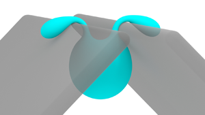
Consider a single freely suspended, neutrally buoyant drop within a uniform far-field flow, approaching one or more complex-shaped particles fixed in space; Newtonian quasi-steady Stokes flow is assumed inside and outside the drop. The boundary-integral formulation assumes all surfaces have smoothly varying normals. Still, the class of smooth, closed surfaces is an infinite parameter space; herein we focus on rounded cylinders (capsules) and thin, rounded cuboids (plates), as models for common experimental set-ups as well as fibrous and other porous media. Several well-defined asymmetric constrictions and particles are also considered (§§ 5.4 and 5.5), in order to elicit more complex drop behaviour. For spheres, capsules and derivative particles, the characteristic length  $L$ is a radius of the solid particle (figure 1). In the case of rounded plates,
  $L$ is defined as the gap between two plates forming a constriction. The drop centre is initially placed
  $10L$ upstream from the particles’ basal plane, unless noted otherwise. The ratio of the drop viscosity (
 $\mu _d$) and external medium viscosity (
 $\mu _e$) is
  $\lambda = \mu _d/\mu _e$ and the uniform far-field velocity carrying the drop towards the constriction is
  $\boldsymbol {u}_{\infty }$. The capillary number is defined as
 \begin{equation} Ca = \frac{\mu_e |\boldsymbol{u}_{\infty}|}{\sigma} \frac{\tilde{a}}{L}, \end{equation}
where  $\tilde {a}$ is the non-deformed drop radius and
  $\sigma$ is the constant surface tension of the surfactant-free drop interface.

Figure 1. Particle shapes used to construct constrictions (as well as individual-particle obstacles, in the case of the capsule). The capsule is a cylinder capped with hemispheres on either end. The half-capsule is a capsule cut in half lengthwise, and then capped with a bevel of radius  $0.2L$. The flat plate is a simple
  $4\times 8\times 0.2L$ rectangular prism with bevelled edges. Particles not shown to scale.
Other important metrics used to quantify drop dynamics include the drop–particle gap and the drop velocity. The gap between the drop and each solid particle is defined as the minimum distance between the two mesh polyhedra, assuming flat triangulation. The high-resolution solid-particle meshes were used for increased accuracy of the gap calculation. The instantaneous drop velocity  $\boldsymbol {U}$, defined as the volume-averaged fluid velocity
  $\boldsymbol {u}$ inside the drop, can be calculated through the divergence theorem as
 \begin{equation} \boldsymbol{U} = \langle \boldsymbol{u} \rangle = \frac{1}{\tilde{V}} \int_{\tilde{S}}(\boldsymbol{u}\boldsymbol{\cdot}\boldsymbol{n}) (\boldsymbol{x}-\tilde{\boldsymbol{x}}^{c})\, \textrm{d} S, \end{equation}
where  $\tilde {V}$ is the drop volume,
  $\boldsymbol {n}$ are outward surface unit normals at points
  $\boldsymbol {x}$ on the surface and
  $\tilde {\boldsymbol {x}}^{c}$ is the drop centroid. In what follows,
  $U$ is the component of
  $\boldsymbol {U}$ along
  $\boldsymbol {u}_{\infty }$.
The solid particles used to build constrictions are shown in figure 1. A capsule, or spherocylinder, is a round cylinder capped with hemispheres, with a maximum dimension  $\mathcal {L}$. A range of lengths
  $\mathcal {L}$ are tested; however, a default of
  $\mathcal {L}=6$ is used for parametric studies. A half-capsule is constructed by dividing a capsule (
 $\mathcal {L}=6$) in half lengthwise, and capping the resulting sharp edge with a circular bevel of radius
  $0.2L$. As shown below, constrictions are formed by two parallel capsules or half-capsules, separated by a minimum gap of
  $0.5L$. A plate is a rectangular prism bevelled to preserve its original maximal dimensions. The plate dimensions are
  $4\times 8\times 0.2L$, where
  $L$ is the minimum distance between two plates forming a constriction. In addition to satisfying the assumption of smooth surfaces in the boundary-integral formulation below, rounding sharp edges on solids also serves to preserve a finite lubrication layer between the drop and solid and prevent excessive local deformation of the drop interface.
3. Desingularized boundary-integral formulation
The present boundary-integral formulation for drops interacting with arbitrary smooth particles utilizes the suite of desingularization methods detailed by Zinchenko & Davis (Reference Zinchenko and Davis2006), but replaces all involved analytical desingularization integrals with semi-analytical or numerical integrals. The semi-analytical desingularization for axisymmetric particles and the numerical method for arbitrary surfaces are outlined in § 4. The Hebeker representation is used for each solid-particle contribution as a linear combination of single-layer and double-layer potentials, and the interfacial stress contribution is desingularized for both drop self-interactions and drop–solid contributions. The resulting Fredholm integral equations of the second kind are well behaved for tight-squeezing drops, for which drop–solid separation distances can be several orders of magnitude smaller than the system's characteristic length.
Let  $\tilde {N}$ be, for generality, the number of drops in the system (with the same viscosity ratio
  $\lambda$),
  $\tilde {S}$ be the surfaces of these drops,
  $\hat {N}$ be the number of solid particles and
  $\hat {S}$ be the surfaces of these particles. The no-slip boundary condition
  $\boldsymbol {u} = \boldsymbol {0}$ is enforced for the fluid velocity on the solid boundaries. The far-field velocity
  $\boldsymbol {u}_{\infty }(\boldsymbol {y})$ away from the particles and drops can be an arbitrary Stokes flow (although a uniform
  $\boldsymbol {u}_{\infty }$ was assumed in the present simulations). Standard Wielandt's deflation is beneficial to avoid ill conditioning at extreme viscosity ratios. To this end, the system is cast in terms of
  $\boldsymbol {w}=\boldsymbol {u}-\kappa \boldsymbol {u}'$, where
  $\kappa = (\lambda -1)/(\lambda +1)$ and
  $\boldsymbol {u}'$ is the rigid-body projection (see below) of
  $\boldsymbol {u}$ on a drop surface. At every time step, the following system of equations is solved for modified interface velocity
  $\boldsymbol {w}$ on drops and Hebeker density
  $\boldsymbol {q}$ on solid surfaces (Zinchenko & Davis Reference Zinchenko and Davis2006):
 \begin{align} \boldsymbol{w}(\boldsymbol{y}) &= \frac{2\boldsymbol{F}(\boldsymbol{y})}{\lambda+1} + \kappa \left[ 2 \sum_{\beta =1}^{\tilde{N}} \int_{\tilde{S}_\beta} \boldsymbol{w}(\boldsymbol{x}) \boldsymbol{\cdot} \boldsymbol{\tau} (\boldsymbol{r}) \boldsymbol{\cdot} \boldsymbol{n}(\boldsymbol{x}) \,\mbox{d} S_x - \boldsymbol{w}'(\boldsymbol{y}) + \frac{\boldsymbol{n}(\boldsymbol{y})}{\tilde{S}_\alpha} \int_{\tilde{S}_\alpha} \boldsymbol{w} \boldsymbol{\cdot} \boldsymbol{n} \,\mbox{d} S \right] \nonumber\\ &\quad +\frac{2}{\lambda + 1} \sum_{\beta =1}^{\hat{N}} \int_{\hat{S}_\beta} \boldsymbol{q}(\boldsymbol{x}) \boldsymbol{\cdot} [2\boldsymbol{\tau}(\boldsymbol{r})\boldsymbol{\cdot}\boldsymbol{n}(\boldsymbol{x}) + \eta \textbf{G}(\boldsymbol{r})]\,\mbox{d} S_x \end{align}
for  $\boldsymbol {y} \in \tilde {S}_\alpha \ (\alpha =1\cdots \tilde {N})$ and
 \begin{align} \boldsymbol{q}(\boldsymbol{y}) &= \boldsymbol{F}(\boldsymbol{y}) + (\lambda-1) \sum_{\beta =1}^{\tilde{N}} \int_{\tilde{S}_\beta} \boldsymbol{w}(\boldsymbol{x}) \boldsymbol{\cdot} \boldsymbol{\tau} (\boldsymbol{r}) \boldsymbol{\cdot} \boldsymbol{n}(\boldsymbol{x}) \,\mbox{d} S_x \nonumber\\ &\quad +\sum_{\beta =1}^{\hat{N}} \int_{\hat{S}_\beta} \boldsymbol{q}(\boldsymbol{x}) \boldsymbol{\cdot} [2\boldsymbol{\tau}(\boldsymbol{r}) \boldsymbol{\cdot}\boldsymbol{n}(\boldsymbol{x}) + \eta \textbf{G}(\boldsymbol{r})]\,\mbox{d} S_x \end{align}
on solid-particle surfaces ( $\boldsymbol {y}\in \hat {S}_{\alpha },\ \alpha =1\cdots \hat {N}$). Here,
  $\mbox {d} S_x$ is the surface element for the integration point
  $\boldsymbol {x}$,
  $\boldsymbol {r} = \boldsymbol {x}-\boldsymbol {y}$,
  $\boldsymbol {n}$ is the unit normal to a surface,
  $\eta >0$ is the Hebeker parameter (the choice of
  $\eta$ affects the algorithm robustness, but not the solution upon numerical convergence) and prime indicates rigid-body projection. The latter is calculated as
  $\boldsymbol {w}'(\boldsymbol {y})=\boldsymbol {A}+\boldsymbol {B}\times (\boldsymbol {y}-\tilde {\boldsymbol {x}}^{c}_\alpha )$, where
  $\boldsymbol {A}$ is the average of
  $\boldsymbol {w}$ over the drop surface
  $\tilde {S}_{\alpha }$,
  $\tilde {\boldsymbol {x}}^{c}_{\alpha }$ is the drop surface centroid and the vector
  $\boldsymbol {B}$ is calculated from the solution of a
  $3\times 3$ system with a positive–definite matrix (Zinchenko, Rother & Davis Reference Zinchenko, Rother and Davis1997):
 \begin{equation} \left\{ \int_{\tilde{S}_\alpha} [(\boldsymbol{x}-\tilde{\boldsymbol{x}}^{c}_\alpha)^{2}\boldsymbol{I}- (\boldsymbol{x}-\tilde{\boldsymbol{x}}^{c}_\alpha)(\boldsymbol{x}-\tilde{\boldsymbol{x}}^{c}_\alpha)]\,\mbox{d} S \right\} \cdot \boldsymbol{B} = \int_{\tilde{S}_\alpha} (\boldsymbol{x}-\tilde{\boldsymbol{x}}^{c}_\alpha) \times \boldsymbol{w} \,\mbox{d} S. \end{equation}
 The single-layer terms containing the Hebeker parameter  $\eta$ serve to complete the range of boundary-integral operators; without these terms, the double-layer boundary-integral contribution could not accommodate non-zero hydrodynamic forces or torques acting on the solid particles. The inhomogeneous term is
 \begin{equation} \boldsymbol{F}(\boldsymbol{y}) = \boldsymbol{u}_\infty(\boldsymbol{y}) + \frac{2\sigma}{\mu_e}\sum_{\beta =1}^{\tilde{N}} \int_{\tilde{S}_\beta} k(\boldsymbol{x}) \boldsymbol{n}(\boldsymbol{x}) \boldsymbol{\cdot} \textbf{G}(\boldsymbol{r}) \,\mbox{d} S_x, \end{equation}
where  $k$ is the mean surface curvature
  $k(\boldsymbol {x})=(k_1+k_2)/2$, with
  $k_1$,
  $k_2$ being the principal curvatures at
  $\boldsymbol {x}$. Normal vectors and curvatures are calculated using the high-order method introduced in Zinchenko & Davis (Reference Zinchenko and Davis2006), which provides accurate values even for very elongated drops; a validation of this method is provided in appendix C. Finally,
  $\textbf {G}(\boldsymbol {r})$ and
  $\boldsymbol {\tau }(\boldsymbol {r})$ are the free-space Green tensor and the corresponding fundamental stresslet, respectively
 \begin{equation} \textbf{G}(\boldsymbol{r}) ={-}\frac{1}{8{\rm \pi}}\left[ \frac{\boldsymbol{I}}{r} + \frac{\boldsymbol{r}\boldsymbol{r}}{r^{3}}\right], \quad \boldsymbol{\tau}(\boldsymbol{r}) = \frac{3}{4{\rm \pi}}\frac{\boldsymbol{r}\boldsymbol{r}\boldsymbol{r}}{r^{5}}. \end{equation}
 Despite the singularities in the kernels (3.5a,b) at  $r\to 0$, all self-integrals (3.1), (3.2) and (3.4) (i.e. when the observation point
  $\boldsymbol {y}$ lies on an integration surface) are convergent due to
  $\boldsymbol {\tau } \boldsymbol {\cdot } \boldsymbol {n} =O(1/r)$ (cf.
  $|\boldsymbol {\tau }|{\sim }1/r^{2}$). However, the singular and near-singular behaviour of the integrands (for droplet–droplet, droplet–particle and particle–particle interactions) must be alleviated, as described in the next section, for a successful numerical solution. After such desingularizations, (3.1) and (3.2) are solved by Generalized Minimal Residual (GMRES) iterations, and the drop node positions are time integrated using a second-order Runge–Kutta scheme. The time step is determined by the empirical formula introduced by Zinchenko & Davis (Reference Zinchenko and Davis2005)
 \begin{equation} {\rm \Delta} t = \frac{K_{{\rm \Delta} t} \mu_e}{\sigma} \min ({\rm \Delta} x, 0.7{\rm \Delta} x_2), \end{equation}
where
 \begin{equation} {\rm \Delta} x_2 = \min_{i,j} \left\Vert \boldsymbol{x}_j - \boldsymbol{x}_i \right\Vert,\quad \boldsymbol{x}_i \in \tilde{S},\enspace \boldsymbol{x}_j \in \hat{S} \end{equation}
is the minimum distance between mesh nodes on the drop and a solid surface, but excluding pairs ( $i$,
$i$, $j$) for which
  $\boldsymbol {x}_j$ is the solid-particle node closest to
  $\boldsymbol {x}_i$, or
  $\boldsymbol {x}_i$ is the drop node closest to
  $\boldsymbol {x}_j$. This exclusion is possible due to near-singularity subtractions, and the coefficient 0.7 is an empirical correction. A value of
  $K_{{\rm \Delta} t}=8.75$ was found to be economical and stable over a wide range of parameters. Mesh quality (roughly, the absence of nearly degenerate mesh triangles) is maintained using passive mesh stabilization, as in Zinchenko & Davis (Reference Zinchenko and Davis2006), and in some cases the customizable remeshing technique described in § 4.
4. Numerical method
4.1. General desingularization formulae
A repository of desingularization techniques that permit stable hydrodynamic interactions between drops and solid particles is provided by Zinchenko & Davis (Reference Zinchenko and Davis2006), including drop and solid self-interactions, solid–solid interaction, solid–drop and drop–solid contributions. In certain cases (solid self-interaction, solid–solid interaction and solid–drop contributions), additional integrals appear during the subtraction procedure that must be calculated with near-analytical accuracy to facilitate tight-squeezing simulations. The complete desingularization expressions and relevant ‘high-accuracy integrals’ in each case are listed below.
For solid self-interaction ( $\boldsymbol {y}\in \hat {S}_\alpha$), singularity subtraction is provided by
 \begin{align} & \int_{\hat{S}_\alpha} \boldsymbol{q}(\boldsymbol{x})\boldsymbol{\cdot}[2\boldsymbol{\tau} (\boldsymbol{r})\boldsymbol{\cdot}\boldsymbol{n}(\boldsymbol{x})+ \eta \boldsymbol{G}(\boldsymbol{r})] \,\mbox{d} S_x \nonumber\\ &\quad =\boldsymbol{q}(\boldsymbol{y}) + \int_{\hat{S}_\alpha} [\boldsymbol{q}(\boldsymbol{x})-\boldsymbol{q}(\boldsymbol{y})] \boldsymbol{\cdot}[2\boldsymbol{\tau}(\boldsymbol{r}) \boldsymbol{\cdot}\boldsymbol{n}(\boldsymbol{x})+\eta \boldsymbol{G}(\boldsymbol{r})] \, \mbox{d} S_x + \eta\boldsymbol{q}(\boldsymbol{y})\int_{\hat{S}_\alpha} \boldsymbol{G}(\boldsymbol{r}) \,\mbox{d} S_x, \end{align}
where the final integral on the right-hand side of (4.1) must be computed with high accuracy.
Solid–solid interactions are transformed slightly differently, but contain the same integral requiring near-analytical treatment
 \begin{align} & \int_{\hat{S}_\beta} \boldsymbol{q}(\boldsymbol{x})\boldsymbol{\cdot}[2\boldsymbol{\tau} (\boldsymbol{r})\boldsymbol{\cdot}\boldsymbol{n}(\boldsymbol{x})+ \eta \boldsymbol{G}(\boldsymbol{r})] \,\mbox{d} S_x \nonumber\\ &\quad =\int_{\hat{S}_\beta} [\boldsymbol{q}(\boldsymbol{x})-\boldsymbol{q}(\boldsymbol{x}^{*})] \boldsymbol{\cdot}[2\boldsymbol{\tau}(\boldsymbol{r})\boldsymbol{\cdot}\boldsymbol{n} (\boldsymbol{x})+\eta \boldsymbol{G}(\boldsymbol{r})] \,\mbox{d} S_x + \eta\boldsymbol{q}(\boldsymbol{x}^{*})\int_{\hat{S}_\beta}\boldsymbol{G}(\boldsymbol{r}) \,\mbox{d} S_x, \end{align}
where  $\boldsymbol {x}^{*} = \boldsymbol {x}^{*}(\boldsymbol {y},\beta )$ is the mesh node on
  $\hat {S}_\beta$ closest to
  $\boldsymbol {y}\in \hat {S}_\alpha \neq \hat {S}_\beta$.
Likewise, the single-layer part of the solid–drop contribution utilizes a simple regularization also involving  $\boldsymbol {G}(\boldsymbol {r})$
 \begin{equation} \int_{\hat{S}_\beta} \boldsymbol{q}(\boldsymbol{x})\boldsymbol{\cdot} \boldsymbol{G}(\boldsymbol{r})\,\mbox{d} S_x = \int_{\hat{S}_\beta} [\boldsymbol{q}(\boldsymbol{x})-\boldsymbol{q}(\boldsymbol{x}^{*})] \boldsymbol{\cdot}\boldsymbol{G}(\boldsymbol{r})\,\mbox{d} S_x + \boldsymbol{q}(\boldsymbol{x}^{*}) \int_{\hat{S}_\beta} \boldsymbol{G}(\boldsymbol{r})\,\mbox{d} S_x. \end{equation}
 Finally, the high-order near-singularity subtraction used for the solid–drop double-layer contribution was found to be especially critical for stable tight-squeezing simulations. To this end, for  $\boldsymbol {y}$ on a drop surface
  $\tilde {S}_{\alpha }$ and its nearest mesh node
  $\boldsymbol {x}^{*}$ on a solid surface
  $\hat {S}_{\beta }$, the density function
  $\boldsymbol {q}(\boldsymbol {x})$ near
  $\boldsymbol {x}^{*}$ is approximated by
  $\boldsymbol {q}(\boldsymbol {x^{*}})$ plus a linear function
  $\mathscr {L}(\boldsymbol {x}-\boldsymbol {x}^{*})$; the coefficients of the linear form
  $\mathscr {L}$ are found by least-squares fitting to the values of
  ${\rm \Delta} \boldsymbol {q}(\boldsymbol {x}^{j})=\boldsymbol {q}(\boldsymbol {x}^{j})-\boldsymbol {q}(\boldsymbol {x}^{*})$ in the solid mesh nodes
  $\boldsymbol {x}^{j}$ directly connected to
  $\boldsymbol {x}^{*}$. Subtracting
  $\boldsymbol {q}(\boldsymbol {x}^{*})+\mathscr {L}(\boldsymbol {x}-\boldsymbol {x}^{*})$ from
  $\boldsymbol {q}(\boldsymbol {x})$ completely desingularizes the double-layer part of the solid–drop contribution in (3.1), but gives rise to added-back integrals, which need to be handled either analytically (possible only for a few shapes), or, in general, numerically with high accuracy. This desingularization can be written as
 \begin{align} & \int_{\hat{S}_\beta} \boldsymbol{q}(\boldsymbol{x})\boldsymbol{\cdot}\boldsymbol{\tau}(\boldsymbol{r}) \boldsymbol{\cdot}\boldsymbol{n}(\boldsymbol{x}) \,\mbox{d} S_x \nonumber\\ &\quad =\int_{\hat{S}_\beta}\left[ \boldsymbol{q}(\boldsymbol{x})-\boldsymbol{q}(\boldsymbol{x}^{*})- \sum_{j\in\mathcal{A}(\boldsymbol{x}^{*})} (\boldsymbol{c}_j \boldsymbol{\cdot}(\boldsymbol{x}-\boldsymbol{x}^{*})){\rm \Delta}\boldsymbol{q}(\boldsymbol{x}^{j})\right] \boldsymbol{\cdot} \boldsymbol{\tau}(\boldsymbol{r}) \boldsymbol{\cdot} \boldsymbol{n}(\boldsymbol{x}) \,\mbox{d} S_x \nonumber\\ &\qquad +\sum_{j\in\mathcal{A}(\boldsymbol{x}^{*})} [\boldsymbol{c}_j{\rm \Delta}\boldsymbol{q}(\boldsymbol{x}^{j})]\boldsymbol{\cdot}\frac{3}{4{\rm \pi}} \int_{\hat{S}_\beta} \frac{[\boldsymbol{r}\boldsymbol{\cdot}\boldsymbol{n}(\boldsymbol{x})] \boldsymbol{r}\boldsymbol{r}\boldsymbol{r}}{r^{5}}\,\mbox{d} S_x, \end{align}
where  $\mathcal {A}(\boldsymbol {x}^{*})$ is the set of nodes directly connected to
  $\boldsymbol {x}^{*}$; the vector coefficients
  $\boldsymbol {c}_j$ depend only on the local mesh geometry near
  $\boldsymbol {x}^{*}$ and are pre-calculated as detailed in § 3 of Zinchenko & Davis (Reference Zinchenko and Davis2006).
So, high-accuracy computation of three integral terms is required. Up to a factor, we denote these terms as
 \begin{gather} G_1(\boldsymbol{y},\beta) \equiv \int_{\hat{S}_\beta}\frac{1}{r}\,\mbox{d} S_x,\quad \boldsymbol{G}_2(\boldsymbol{y},\beta) \equiv \int_{\hat{S}_\beta}\frac{\boldsymbol{r}\boldsymbol{r}}{r^{3}}\,\mbox{d} S_x, \end{gather}
 \begin{gather}\boldsymbol{\varPsi}(\boldsymbol{y},\beta) \equiv \int_{\hat{S}_\beta}\frac{(\boldsymbol{r}\boldsymbol{\cdot}\boldsymbol{n}(\boldsymbol{x})) \boldsymbol{r}\boldsymbol{r}\boldsymbol{r}}{r^{5}}\,\mbox{d} S_x. \end{gather}
It is advantageous that the second-rank tensor  $\boldsymbol {G}_2$ and the third-rank tensor
  $\boldsymbol {\varPsi }$ are fully permutable in their indices, thus reducing the amount of work to calculate these tensors.
4.2. Semi-analytical desingularization for axisymmetric particles
Axisymmetric particles permit semi-analytical calculation of the integrals (4.5a,b) and (4.6), by closed-form azimuthal integration around the particle axis of rotation, with external numerical integration along the particle half-contour. This kind of approach has been widely used in axisymmetric boundary-integral solutions (e.g. Rallison & Acrivos Reference Rallison and Acrivos1978; Lee & Leal Reference Lee and Leal1982; Davis Reference Davis1999; Ratcliffe et al. Reference Ratcliffe, Zinchenko and Davis2010) by reducing the azimuthal integration to elliptic integrals (as discussed in detail by Pozrikidis Reference Pozrikidis1992). In the present 3-D work, analytical azimuthal integration for the high-order subtraction tensor (4.6) is a more cumbersome, but still very efficient approach. As shown in figure 2, a representative integration circumference  $C$ is the perimeter of a representative disk of radius
  $\rho$, a sufficient number
 ![]() of which form an approximation to the axisymmetric volume. The surface integral of a function
of which form an approximation to the axisymmetric volume. The surface integral of a function  $f(\boldsymbol {x})$ is simply
 \begin{equation} \int_{\hat{S}_\beta} f(\boldsymbol{x})\,\mbox{d} S_x = \int \rho\,\mbox{d}s \left[\oint_{C}f(\boldsymbol{x})\,\mbox{d} \varPsi \right], \end{equation}
where  $\varPsi \in [-{\rm \pi} ,{\rm \pi} ]$ is the azimuthal angle of rotation around the particle axis, and
  $\mbox {d}s$ is the contour length element along the particle's half-contour.

Figure 2. An axisymmetric particle oriented as a surface of revolution  $\hat {S}_\beta$ around the
  $z$-axis. The single- and double-layer contributions of circular segments can be calculated analytically using elliptic integrals. For a given representative circle
  $C$, the origin
  $\boldsymbol {O}$ may be placed at its centre, with the
  $x$-axis in plane but oriented away from the observation point
  $\boldsymbol {x}_0$. Cylindrical coordinates (
 $\rho ,\psi ,z$) are used for deriving elliptic integral calculations.
Now, we outline derivations for closed-form expressions for the integrals (4.5a,b) and (4.6) over a representative circumference  $C$, in terms of complete elliptic integrals of the first and second kind. Let the origin
  $\boldsymbol {O}$ of the temporary coordinate system
  $(\rho \cos {\psi },\rho \sin {\psi },z)$ be at the centre of
  $C$, with its axis of revolution along the
  $z$-axis (figure 2). Without loss of generality, the
  $x$-axis can be defined as antiparallel to the shortest vector from the
  $z$-axis to the observation point
  $\boldsymbol {x}_0$. The observation point is then
  $\boldsymbol {x}_0 = (-\rho _0,0,z_0)$ and the vector
  $\boldsymbol {r}=\boldsymbol {x}-\boldsymbol {x}_0$ between
  $\boldsymbol {x}_0$ and a integration point
  $\boldsymbol {x}$ on
  $C$ is given by
 \begin{equation} \boldsymbol{r} = (\rho\cos{\psi}+\rho_0,\rho\sin{\psi},z-z_0), \end{equation}
and
 \begin{align} r^{2} = \left[(\rho+\rho_0)^{2}+(z-z_0)^{2}\right]\left[1-k^{2}\sin^{2}{\frac{\psi}{2}}\right],\quad \mbox{where}\ k^{2} = \frac{4\rho\rho_0}{(\rho+\rho_0)^{2}+(z-z_0)^{2}}. \end{align}
 The simplest contour integral over  $C$ relevant to computing
  $G_1$ may be expressed as
 \begin{equation} \int_{-{\rm \pi}}^{\rm \pi} \frac{1}{r} \mbox{d} \psi = c_0\int_{-{\rm \pi}}^{\rm \pi} \left[1-k^{2}\sin^{2}{\frac{\psi}{2}}\right]^{{-}1/2}\mbox{d} \psi = 4c_0F, \end{equation}
where  $c_0 = ((\rho +\rho _0)^{2}+(z-z_0)^{2})^{-1/2}$ and
  $F$ is the complete elliptic integral of the first kind with modulus
  $k$. The relevant integrals over
  $C$ for
  $\boldsymbol {G}_2$ and
  $\boldsymbol {\varPsi }$ can be derived in a similar manner and final expressions are provided in appendix A. Once
  $\boldsymbol {G}_2$ and
  $\boldsymbol {\varPsi }$ are computed in the special coordinate basis defined above, they are then transformed by usual tensor transformation rules to the global basis used in the squeezing simulation.
The present semi-analytical approach results in very fast and accurate calculation of single- and double-layer desingularization integrals (4.5a,b) and (4.6) for axisymmetric particles. Surface integrals calculated by (4.7) converge quickly with respect to ![]() (with second-order Euler external integration). For example, using a capsule (
(with second-order Euler external integration). For example, using a capsule ( $\mathcal {L}=6$) as a test particle and an observation point
  $0.01L$ away from the cylindrical section of particle surface, all
  $\boldsymbol {\varPsi }$ terms agree to within at least the fifth decimal point for
 ![]() values of 1000 and 10 000. The former corresponds to a representative disk width of 0.006. Further convergence tests and comparisons with the multimesh method are provided in § 5.1.
values of 1000 and 10 000. The former corresponds to a representative disk width of 0.006. Further convergence tests and comparisons with the multimesh method are provided in § 5.1.
4.3. Multimesh desingularization
Desingularization for arbitrarily shaped particles can be achieved with direct numerical calculation of  $G_1$,
  $\boldsymbol {G}_2$ and
  $\boldsymbol {\varPsi }$ (4.5a,b) and (4.6), if sufficiently high resolution meshes are used to discretize these surface integrals. Note that this ‘multimesh desingularization method’ still requires particles to have smoothly varying normals (i.e. to be Lyapunov surfaces). Extremely high resolutions are required for single- and double-layer contributions to approach exact values, in order to accurately and stably reproduce analytical or semi-analytical tight-squeezing results. Due to the singular nature of the integrals, accuracy is more sensitive to mesh resolution as the observation point approaches the particle surface; therefore, a hierarchy of embedded meshes is used for multimesh desingularization.
Two high-resolution auxiliary meshes are used to compute the desingularization integrals. The first high-resolution mesh typically has four times more triangles than the basic mesh used for BIM calculations. The second is an ultra-high-resolution mesh, typically 64 times denser than the basic mesh, as shown in figure 3(a,b). For particles with higher surface area, the ultra-high-resolution mesh may have in excess of 2.5 million triangles. Therefore, the two meshes are chained to each other: the indices of the 16 ultra-high-resolution triangles within each high-resolution triangle are pre-calculated and stored. In contrast to boundary-integral calculations for desingularized terms on the basic mesh, with mesh triangle contribution reassigned to vertices (a procedure due to Rallison (Reference Rallison1981) used in many prior simulations), such reassignment is disadvantageous for multimesh calculations of the desingularization tensors. A primitive form is used instead:
 \begin{equation} \int_{\hat{S}_\beta} f(\boldsymbol{x}) \,\mbox{d}S_x \approx \sum_i f(\boldsymbol{x}_i){\rm \Delta} S_i, \end{equation}
where the summation is over all triangles for a given triangulation of the surface  $\hat {S}_\beta$,
  $\boldsymbol {x}_i$ is the triangle centroid and
  ${\rm \Delta} S_i$ is the flat triangle area. This form makes it straightforward to use one mesh within a given cutoff distance
  $r_c$ from the observation point, and another one beyond that radius, as illustrated in figure 3(c). Specifically, the distance between a given observation point
  $\boldsymbol {x}_0$ and high-resolution triangle is determined using the triangle centroid. If this distance is greater than the prescribed distance cutoff
  $r_c$, then this triangle is used as an area element
  ${\rm \Delta} S_i$ of the surface integral in (4.11). Otherwise, the 16 corresponding ultra-high-resolution triangles are substituted to represent this triangle contribution to (4.11). The desingularization integrals for solid self-interaction and solid–solid interactions are calculated only once at the start of each simulation, so a high distance cutoff (
 $r_c=1.0L$) was used with a negligible penalty on total CPU time. The solid–drop contribution to the desingularization integrals is computed outside of GMRES iterations, but still represents the slowest operation of the multimesh method. A distance cutoff of
  $r_c=0.4L$ for the solid–drop contribution was found sufficient to stably model tight-squeezing or trapped drops with an accuracy approaching that of analytical methods, as discussed in § 5.1.

Figure 3. Solid-particle meshes used for the  $\mathcal {L}=4$ capsule by the multimesh desingularization method. (a) The high-resolution (
 $\hat {N}_{\triangle }=52\ \text {K}$) and ultra-high-resolution (
 $\hat {N}_{\triangle }=840\ \text {K}$) meshes used for numerical desingularization. The additional edges of the ultra-high-resolution mesh are coloured cyan. (b) The basic mesh (
 $\hat {N}_{\triangle }=13\ \text {K}$) used by the BIM simulation for desingularized terms. (c) A given observation point
  $\boldsymbol {x}_0$ calculates per-triangle values from the ultra-high-resolution mesh within a cutoff
  $r_c$.
Several technical issues arise due to the requirements of (i) quality meshing of arbitrary shapes, (ii) obtaining machine precision for node positions, (iii) memory requirements of ultra-high-resolution meshes and (iv) mesh chaining. An approximate mesh for each particle resolution was created using the powerful open-source software Blender, which has no limitation on mesh size and can easily handle meshes with  $N_{\triangle }>2.5\ \mbox {M}$, but uses single-precision floating-point format for coordinates (which may create unwanted numerical errors in tight-squeezing simulations). After node positions and connectivity are exported from Blender, coordinates are read into the BIM program and adjusted to double precision according to piecewise analytical functions that define a given particle shape. Similarly, the surface normals at each node are calculated using analytical formulae for a particular surface. A more general approach would be to use just node positions on the solid surfaces and calculate the normals by the same tools as we employ for the triangulated drop surface (appendix C), but such generality was not pursued in the present calculations. Due to memory considerations, only one instance of each desingularization mesh is saved in memory, and is translated and/or mirrored (see § 4.4) during calculations over a given particle. Finally, an efficient algorithm was written to chain two meshes to each other, i.e. to determine which ultra-high-resolution triangles lie within each high-resolution triangle. The algorithm requires knowledge only of the node positions and connectivity of the two meshes, assuming every high-resolution node coincides with an ultra-high-resolution node. Briefly, coinciding nodes between the meshes are determined by position, and a nearby ultra-high-resolution triangle is associated with a given high-resolution triangle if its centroid (projected along the surface normal) lies within the perimeter of the high-resolution triangle.
4.4. Additional numerical considerations
Two configurations, drop flow around a single capsule and between two flat plates, presented particular challenges regarding numerical stability and drop mesh quality. A useful extension of the commonly used triangle subdivision scheme introduced by Cristini, Bławzdziewicz & Loewenberg (Reference Cristini, Bławzdziewicz and Loewenberg2001) was developed, which is particularly effective when remeshing contiguous regions on a drop. The simple idea is, given a list of all triangles to be subdivided within a given region, a uniform mesh four times denser than the original can immediately result, by adding nodes at all edge midpoints and appropriately connecting them (see appendix B). Connectivity around the perimeter of this region can also be determined simply, e.g. in the manner of Cristini et al. (Reference Cristini, Bławzdziewicz and Loewenberg2001) (§ A.1.2. therein). Occasional node addition on regions of contiguous triangles had two benefits. First, a much cleaner mesh immediately resulted, such that further relaxation tangential to the drop surface was unneeded. Second, updating the mesh topology was required much less often, resulting in a more efficient algorithm. For example, in the case of a single drop approaching a single fibre, passive mesh stabilization alone (in the form of Zinchenko & Davis Reference Zinchenko and Davis2006) was found to be inadequate due to the large drop deformation. This simulation was greatly extended by defining an upper limit on triangle area, and whenever this limit was reached, executing node addition on all triangles within a cutoff distance of the triangle with maximal area. In this case, similar simulation times were reached by actively redistributing nodes using an advanced potential energy function (Zinchenko & Davis Reference Zinchenko and Davis2013). A fourth-order variation of the best-paraboloid method (Zinchenko & Davis Reference Zinchenko and Davis2006) was used to used to choose coordinates for the inserted nodes. Including the second- and third-level neighbours in the fit improved the local curvatures at inserted nodes, in areas of both low and high curvature, and allowed the simulation to continue stably without the intermediate step of relaxing inserted nodes. Note that a four-times-denser triangle mesh corresponds to mesh edges one half their original length; the tighter Courant stability limitation on the time step was not prohibitive for any systems presented herein. To maintain mesh quality on the whole drop, passive mesh stabilization (Zinchenko & Davis Reference Zinchenko and Davis2006) is also enforced for all nodes at every time step.
The above ‘coordinated adaptive remeshing’ scheme was extended to allow added nodes to be subsequently removed. In the case of a drop squeezing between thin plates, especially at low capillary numbers, it was necessary to include a spatially dependent remeshing scheme for the drop surface, with criteria defined to increase mesh resolution within near-contact regions of the drop (figure 4a,b). In this case, the drop does not experience particularly high deformation or curvatures, yet mesh stability greatly benefits from increased resolution in specific regions. This criteria-based local remeshing is achieved by remembering the original mesh connectivity, restoring it and re-evaluating the given criteria for refinement (every so many time steps). Therefore, the region of higher mesh resolution shown in figure 4 remains constant as the drop moves through the constriction. This technique was also necessary for certain half-capsule configurations at low capillary number.

Figure 4. Adaptive mesh schemes for droplet squeezing between plates. (a) Coordinated adaptive meshing of drop surface based on spatial criteria. By storing the original mesh connectivity and re-evaluating the criteria before every remeshing, the region of denser triangulation remains constant as the drop moves through the constriction. (b) Orthogonal view of the same drop, with solid particles hidden.
To prevent symmetry breaking during drop flow, it was necessary that individual solid-particle meshes were made symmetric with respect to all three orthogonal planes that pass through the constriction centre. Also, for the flat-plate system, a fixed adaptive mesh was used for solid particles to increase node density in near-contact regions. Mesh density within two unit lengths of the constriction centre was increased between four and sixteen times, depending on proximity to the constriction centre. This base mesh was refined to create the higher-resolution desingularization meshes. In order to maintain the aforementioned symmetry, while also storing only one copy of the higher-resolution meshes in memory, a value is associated with each particle to indicate whether or not to use the mirror image of a given mesh. Inverting a coordinate is not computationally intensive, allowing for symmetric systems with non-uniform meshes to be efficiently treated within the framework of the multimesh desingularization method.
5. Numerical results
All values from the numerical simulations of drop tight squeezing are reported in non-dimensional form. The characteristic length scale  $L$ is taken as the solid-particle radius
  $\hat {a}$ for capsules and derivative particles; for plates,
  $L$ is the gap between two particles. The velocity and times scales are
  $|\boldsymbol {u}_{\infty }|$ and
  $L/|\boldsymbol {u}_{\infty }|$, respectively. The Hebeker parameter
  $\eta$ in the boundary-integral formulation (3.2) and (3.1) is set to unity. The initial drop shape is spherical and far upstream from the constriction. The definitions of
  $Ca$ and
  $\lambda$ are provided in § 2. Hereafter,
  $\hat {N}_{\triangle }$ and
  $\tilde {N}_{\triangle }$ will refer to the number of triangles in each solid-particle and drop mesh, respectively. For brevity, the abbreviations 5, 8.6 and 11.5 K will be used for
  $\hat {N}_{\triangle } = 5120, 8640, 11\,520$. Higher solid-particle resolutions, whose nodes are typically not uniformly distributed, with be similarly rounded. Unless noted otherwise, the droplet resolution is 11 520 (
 $\tilde {N}_{\triangle }=11.5\ \text {K}$).Three meshes are used for each solid particle in the multimesh desingularization method. Their triangle counts are reported as a multiple of the basic mesh resolution. For example, if the high-resolution mesh is four times denser than the basic mesh, and the ultra-high-resolution is 16 times denser than the high-resolution mesh, all three triangles counts are reported as
  $\hat {N}_{\triangle }=8.6\ \text {K}\times 4\times 16$. Note that, due to the quasi-steady character of the Stokes equations, a drop initially placed at a large, but finite distance upstream, immediately feels the constriction presence, resulting in some deviation of the initial drop velocity from the far-field velocity. It is also worth noting that the disturbance of the far-field velocity field due to the constriction decays slowly, like the inverse distance from the constriction. Still, our initial vertical drop separation from the constriction was large enough, so that increasing the initial vertical drop offset, even twofold from
  $10L$ to
  $20L$ for figure 5(b) below, had no perceptible effect on the whole drop trajectory
  $U(t)$. Of course, such a comparison necessarily required a time shift to match the drop position at the
  $10L$ initial offset between the two simulations.

Figure 5. Convergence testing for the two-capsule constriction ( $\tilde {a}=0.5$,
  $\epsilon =0.5$,
  $\mathcal {L}=6$). (a) Drop velocity when squeezing between two capsules, with respect to solid-particle mesh resolution
  $\hat {N}_{\triangle }$ and number of characteristic disks
 ![]() used for semi-analytical desingularization (
used for semi-analytical desingularization ( $Ca=0.9$,
  $\lambda =4$). (b) Convergence testing at lower viscosity ratio (
 $Ca=1.5$,
  $\lambda =0.25$). At
  $\hat {N}_{\triangle }=20.2K$ the curve for
 ![]() (not shown) is indistinguishable from that for
(not shown) is indistinguishable from that for ![]() .
.
5.1. Convergence with mesh resolution and desingularization methods
Convergence of results for the default capsule length ( $\mathcal {L} = 6$) with respect to solid-particle mesh resolution is shown in figure 5. The
  $\hat {N}_{\triangle } = 35.6\ \text {K}$ mesh utilized adaptive resolution such that the mesh was four times denser within a distance of
  ${\approx }1.4$ from the constriction centre, compared to the
  $\hat {N}_{\triangle } = 20.2\ \text {K}$ mesh. Although
 ![]() was set throughout this work for the number of characteristic disks used in the semi-analytical method (increased for longer capsules to provide an equivalent linear density), figure 5 also shows that half that number produces reasonable results (resulting in an eight-times speedup for desingularization as compared to the multimesh method). Indeed, halving the number of characteristic disks (
was set throughout this work for the number of characteristic disks used in the semi-analytical method (increased for longer capsules to provide an equivalent linear density), figure 5 also shows that half that number produces reasonable results (resulting in an eight-times speedup for desingularization as compared to the multimesh method). Indeed, halving the number of characteristic disks (![]() ) results in agreement near the solution tolerance (
) results in agreement near the solution tolerance ( $1\times 10^{-5}$) for the majority of the squeezing process.
The multimesh implementation was validated against previous results that used analytical desingularization (Zinchenko & Davis Reference Zinchenko and Davis2006), and the multimesh and semi-analytical methods were compared against each other. As shown in figure 6, good agreement is seen for drops squeezing between spheres and spheroidal particles. These two-particle constrictions are prone to symmetry breaking and sensitive to mesh resolutions, so reproducing these tight-squeezing results efficiently and without analytical expressions was unexpected. In particular, the spheroidal system in figure 6(b) is metastable and undergoes symmetry breaking shortly after the minimum drop velocity, with one side of the drop advancing slightly farther downstream than the other, even for the analytical system. For these tests, each higher-resolution mesh was 16 times denser than the previous mesh in the hierarchy. Further increasing these desingularization-mesh densities negatively impacted performance while negligibly affecting droplet dynamics. As shown in figure 9, close agreement was also observed between the multimesh and semi-analytical desingularization techniques for drop squeezing between axisymmetric particles, even for tight squeezing.

Figure 6. Comparison between two types of desingularization methods ( $\tilde {N}_{\triangle }=8.6\ \text {K}$,
  $\hat {N}_{\triangle }=5\ \text {K}\times 16\times 16$). Insets shows snapshot of simulation at
  $U_{min}$. (a) Multimesh and analytical desingularization methods agree well for drop squeezing between two spheres (
 $\epsilon =0.5,\tilde {a}=0.9,Ca=0.63,\lambda =4.0$). (b) Drop squeezing between two parallel oblate spheroids with major and minor axes of 1 and 0.4, respectively (
 $\epsilon =0.5,\tilde {a}=0.75,Ca=0.4,\lambda =1.0$). (c) Absolute error for various methods of calculating the desingularization tensor
  $\boldsymbol {\varPsi }$, as compared to the analytical values for the oblate spheroid shown in (b). The semi-analytical method uses 3000 characteristic disks with adaptive resolution for the disk spacing.
The absolute error of the semi-analytical and multimesh methods for  $\boldsymbol {\varPsi }(\boldsymbol {y})$-calculation is shown in figure 6(c) for an oblate spheroid (one of those in the insert of figure 6b), with the error of the basic mesh (without desingularization) shown for comparison. This error is quantified through root-mean-square deviation of the components
  $\varPsi _{ijk}$ from the analytical values available for this shape (Zinchenko & Davis Reference Zinchenko and Davis2006). Unlike with the cylindrical particles discussed below,
  $\boldsymbol {\varPsi }$ is calculated for observation points
  $\boldsymbol {y}$ near characteristic disks with radii approaching zero, where the characteristic disk radius is indicated by the vertical height of the spheroid in figure 6(c). It was found that a higher density of characteristic disks is required when the radius is near zero. For example, when using 10 000 equally spaced disks for the oblate spheroid (disk width of
  $8\times 10^{-5}$), the semi-analytical method was conspicuously less accurate than the multimesh method, especially near the horizontal axis of figure 6(c). It was necessary to use an adaptive density of disks in this case, whose positions were defined by starting with 1500 points equally spaced on the vertical axis, and determining their (horizontal) location on the spheroid surface using the equation for the spheroid itself. This discretization resulted in 3000 total disks with a minimum width of
  $1.8\times 10^{-7}$ and a maximum width of
  $7.3\times 10^{-3}$ (near the top of the spheroid). The values for the arc lengths
  $\mbox {d}s$ in (4.7) were tabulated beforehand using incomplete elliptic integrals of the second kind. In short, the semi-analytical implementation herein is most efficient, and straightforward, when desingularization accuracy is not critical near the high-curvature solid-particle tips.
5.2. Single capsule
Capsules are presented as a prototype for fibrous material. First, consider a drop approaching a single capsule ( $\mathcal {L}=6$). Patel et al. (Reference Patel, Shaqfeh, Butler, Cristini, Bławzdziewicz and Loewenberg2003) introduced this configuration experimentally, defining the capillary number the same way as herein, and provided boundary-integral results for a drop approaching an infinitely long cylinder. Patel et al. avoided the Stokes paradox (due to an infinite cylinder extent in the third dimension) by using the flow field around the cylinder, which would exist in the absence of the drop, based on the Brinkman equation for an isotropic porous medium, to approximately model the far-field effect of the surrounding fibres in the dilute limit. The boundary-integral problem for the drop was then solved assuming that the drop is immersed into this field, without actual interaction with the cylinder. In the present case, we consider a capsule of finite length only, but solve the problem with full hydrodynamical interaction between the drop and the capsule. The effect of particle length is discussed in more detail in the context of the two-capsule constriction.
Patel et al. (Reference Patel, Shaqfeh, Butler, Cristini, Bławzdziewicz and Loewenberg2003) identified two modes of drop breakup: a grazing mechanism in which drop breakup occurs downstream from the fibre, and hairpin formation when the drop passes around either side, resulting in two bulbous ends, or lobes, connected by a thin filament. The mode of breakup primarily depends on the initial horizontal offset  ${\rm \Delta} y_o$ of the drop centre from the centreline of the capsule. In all cases for the present single-capsule study, system parameters are
  $Ca=3.0, \lambda =1.0$ and
  $\tilde {a}=1.5$, which are typical values used by Patel et al. (Reference Patel, Shaqfeh, Butler, Cristini, Bławzdziewicz and Loewenberg2003), and the drop is initially placed
  $10L$ upstream from the capsule. Hairpin formation was observed for
  ${\rm \Delta} y_o\leq 0.6$, the grazing breakup mechanism was observed for
  ${\rm \Delta} y_o = 0.7$ and the drop remains stable (separation without breakup) for
  ${\rm \Delta} y_o\geq 0.75$. The drop velocity
  $U$ corresponding to various mechanisms is shown vs. time in figure 7(a). Despite the apparent similarity between
  ${\rm \Delta} y_o = 0$ and
  ${\rm \Delta} y_o = 0.1$, overall drop behaviour is highly sensitive to the initial offset. For example, for an offset of
  ${\rm \Delta} y_o = 0.1$, 59 % of the drop (by volume) passes around one side of the capsule. Typical configurations during hairpin formation are shown in figure 7(b). As discussed further below, a large gap (
 ${\approx }0.2$) persists between the filament and the solid particle, even after the majority of drop has passed downstream. It is most noticeable for
  ${\rm \Delta} y_o = 0$ in figure 7(c), that the gap does not go to zero while the drop is able to stay wrapped around the capsule for a long time. The drop diameter, defined as the maximum distance between any points on the drop and normalized by drop radius, is shown in figure 7(d), highlighting the system's sensitivity to initial drop offset.

Figure 7. Droplet flow around a single capsule ( $Ca=3.0, \lambda =1.0, \tilde {a}=1.5, \mathcal {L}=6.0$). (a) Volume-averaged drop velocity
  $vs.$ time as a function of drop offset. The drop remains stable for
  ${\rm \Delta} y_o\geq 0.75$. (b) Typical configurations during the hairpin breakup mechanism. (c) Drop–particle gap as a function of time and drop offset. (d) Drop diameter is sensitive to offset. Length is the maximum distance between any two points on the drop normalized by the undeformed drop radius (curves for
  ${\rm \Delta} y_o = 0.6$ and
  $0.7$ are very similar to
  ${\rm \Delta} y_o = 0.5$).
The lubrication layer between the filament and the fibre influences the drop–particle gap, and this layer is affected by the shape of the filament. This effect is demonstrated using a drop offset of  ${\rm \Delta} y_o = 0.3$ as shown in figure 8(a), which results in a drop shape resembling those observed experimentally by Patel et al. (Reference Patel, Shaqfeh, Butler, Cristini, Bławzdziewicz and Loewenberg2003) (see figure 4 therein). As the filament initially nears the particle face, it spreads axially and an elongated dimple forms along the transverse direction. During this phase, the gap plateaus with respect to time, before decreasing abruptly as the filament thins. This decrease in separation corresponds to the flattening of the dimple into a convex filament. Cross sections of the filament directly above the capsule centre are shown as insets in figure 8(b). The dimple formation shown at
  $t=30$ is dependent on the capsule length; for example, using a capsule of length
  $\mathcal {L}=10$, the filament remains less concave at it approaches the cylindrical surface.

Figure 8. Droplet undergoing large deformation around a capsule ( $Ca=3.0$,
  $\lambda =1.0$,
  $\tilde {a}=1.5$,
  $\mathcal {L}=6.0$). (a) Droplet approaching breakup via the hairpin mechanism. (b) Rate of lubrication layer thinning correlates with the cross-sectional shape of the filament (cross-sectional plane indicated by grey line in (a)).
Our simulations have also revealed the importance of full hydrodynamical interactions for accurate prediction of the drop trajectories around the capsule. When  $\lambda =1$, neglecting the capillary contribution to (3.4) when
  $\boldsymbol {y}$ is on the solid surface, simply makes (3.2) and (3.1) the boundary-integral formulation for the solitary drop immersed in the flow field, which would exist around the solitary capsule. Such an approximation, though, is no longer accurate when the drop comes near a solid surface. For
  ${\rm \Delta} y_o=0.3$, large deviations in the drop shape, position, and velocity between the rigorous and approximate solutions were observed even at
  $t=19$, when the drop is just beginning to wrap around the capsule and the gap is still
  $O(1)$.
5.3. Two-capsule constriction
Consider a drop approaching two parallel capsules separated by a gap  $\epsilon =0.5$, where the non-deformed drop diameter is twice the gap and half the solid-particle diameter. In contrast to drop interactions with a single capsule in unconfined flow, the drop tends to remain compact throughout the squeezing process. An important binary property of this system is whether or not the drop will pass through the constriction; as shown in figure 9(a), the drop is trapped below a critical capillary number. There is excellent agreement between the multimesh (
 $\hat {N}_{\triangle }=20.2\ \text {K}\times 4\times 16$) and semi-analytical (
![]() ) methods, while the semi-analytical calculations were four to eight times faster. As observed for drops squeezing between spheres, the minimum drop–particle gap is almost insensitive to
) methods, while the semi-analytical calculations were four to eight times faster. As observed for drops squeezing between spheres, the minimum drop–particle gap is almost insensitive to  $Ca$ (figure 9b), although this separation remains slightly larger compared to drop squeezing through a three-sphere constriction (Zinchenko & Davis Reference Zinchenko and Davis2006). The tendency of the trailing end of the drop to approach the solid surface more closely as it is exiting, as compared to the majority of the squeezing process (gap decrease
  ${\approx }30\,\%$), is more pronounced for capsules than, e.g. drop squeezing between three spheres. Presumably, the differing nature of the lubrication layers is responsible for this effect; as discussed in § 5.5, the effect is even more pronounced for drops squeezing between flat plates. A snapshot of a supercritical drop when it is approximately centred in the constriction is shown in figure 9(c). The drop profile at the centre of the constriction is outlined by the dashed line in the inset. This dimple in the drop surface is less pronounced during the early and late stages of squeezing. A steady-state trapped drop is also shown from axial and transverse perspectives (figure 9d). The transverse drop profile is approximately circular, as is the case for supercritical drops at a similar position.

Figure 9. Droplet squeezing between two capsules ( $\lambda =4.0$,
  $\tilde {a}=0.5$,
  $\epsilon =0.5$,
  $\mathcal {L}=6.0$). (a) Droplet becomes trapped below a critical capillary number. An agreement is observed between semi-analytical and multimesh methods (
 $\hat {N}_{\triangle }=20.2\ \text {K}\times 4\times 16$). (b) The minimum drop–particle gap is very small for tight-squeezing simulations, and not sensitive to
  $Ca$. (c) Snapshot as drop passes through a two-capsule constriction above
  $Ca_{crit}$. Dashed line in inset outlines drop profile at constriction centre. Two orthogonal views shown. (d) Steady-state drop trapped between two capsules.
Drop squeezing is significantly affected by capsule length, even for long capsules with ends far from the drop. For example, repeating the two-sphere simulation above ( $\epsilon =0.5$,
  $\tilde {a}=0.9$,
  $Ca=0.63$,
  $\lambda =4.0$), but replacing the spheres with capsules of length
  $\mathcal {L}=4$, results in vastly different behaviour. As shown in figure 10(a), the minimum drop velocity
  $U_{min}$ is
  $5\,\%$ of far-field velocity for the two-sphere constriction, whereas the drop becomes trapped in the two-capsule constriction. A parametric study of the effect of cylinder length on droplet trapping was completed at
  $Ca=1.5$,
  $\lambda =4.0$,
  $\tilde {a}=0.5$ and
  $\epsilon =0.5$. One might expect drop velocities to converge relatively quickly after the capsules reach a certain length, due the diminishing end effects. However, a notable difference in drop velocities and squeezing times was observed between
  $\mathcal {L}$ values of 4, 6, 8 and 10, as seen in figure 10(b). This disparity was not significantly alleviated by rescaling the capillary number individually for each system, based on the flow velocity at the centre of the constriction (in an attempt to minimize the effect of the far-field flow
  $\boldsymbol {u}_{\infty }$). The lack of convergence is attributed to variations in the undisturbed (single-phase) flow and can be directly related to the size-effect problems that plague both experimental and numerical studies of the Stokes paradox for flow past long cylinders. For example, Khalili & Liu (Reference Khalili and Liu2017) demonstrate that, for 3-D cylinders, large aspect ratios are required for convergence of results as Reynolds number goes to zero. Furthermore, velocity fields do not converge with decreasing Reynolds number (although unintuitive, this lack of convergence is less surprising given there is no solution for unbounded Stokes flow around an infinite cylinder). Indeed, the aspect ratios of cylinders tractable for this study are orders of magnitude smaller than Khalili & Liu's recommendations for converging velocity and pressure fields. A related work is that of Smith (Reference Smith1990) on the Jeffery paradox (an unintuitive result that involves two cylinders in two dimensions, at least one of which is rotating). Smith came to a similar conclusion that, when attempting to approach this 2-D result using finite 3-D cylinders, cylinder aspect ratios must be many orders of magnitude before end effects become negligible. However, it is not the objective of this work to approximate drop squeezing between infinite cylinders, but rather to model a local environment within fibrous material. Furthermore, a model of porous media that consists of particles in a periodic simulation box, where the flow is either pressure-driven or constant flow rate, is no longer subject to the Stokes paradox, even for effectively infinite cylinders that connect across periodic boundaries. Such a simulation would allow for a more direct comparison to models of flow through porous media, such as the Brinkman equations. The default
  $\mathcal {L}=6$ herein was chosen as a compromise between capsule length and simulation speed.

Figure 10. Effect of capsule aspect ratio on drop squeezing. (a) Cylindrical particles, even at small aspect ratios ( $\mathcal {L}=4$), significantly enhance drop trapping (
 $Ca=0.63$,
  $\lambda =4.0$,
  $\tilde {a}=0.9$,
  $\epsilon =0.5$). (b) Drop trajectories do not converge with respect to capsule length,
  $\mathcal {L}=4$ to
  $10$ (
 $Ca=1.5$,
  $\lambda =4.0$,
  $\tilde {a}=0.5$).
Drop behaviour is also dependent on viscosity ratio  $\lambda$ and non-deformed droplet radius
  $\tilde {a}$. A parametric study of
  $\lambda$ at
  $Ca=1.5$ is shown in figure 11(a). At low
  $\lambda$ and high
  $Ca$, the drop undergoes greater variation in velocity during the squeezing process, and the overall trajectory is more symmetric with respect to time (including the appearance of two global minima for
  $U$). Although squeezing times increase with
  $\lambda$, there is no indication of switching from droplet pass through to trapping within reasonable
  $\lambda$ values. As observed for the three-sphere constriction (Zinchenko & Davis Reference Zinchenko and Davis2006), the drop–particle gap is sensitive to
  $\lambda$, decreasing from about 0.021 for
  $\lambda =10$, to 0.015 for
  $\lambda =0.25$. Drop velocity as a function of
  $Ca$ at low viscosity ratio (
 $\lambda = 0.25$) is shown in figure 11(b) (for comparison at
  $\lambda =4.0$, see figure 9a). Parametric studies for
  $Ca$ also were completed at
  $\lambda =1.0$ and 10; in all cases, the viscosity ratio was not observed to alter pass through
  $vs.$ trapping, as has been noted for drop squeezing between spheres (Zinchenko & Davis Reference Zinchenko and Davis2006). Drop size, in contrast, notably affects
  $Ca_{crit}$. Increasing the drop radius by
  $50\,\%$ results in
  $Ca=1.5$ being subcritical (figure 11c). For
  $\tilde {a}/\epsilon =2.0$, where the drop diameter is four times the gap diameter, the drop must undergo large deformation to pass through. A steady-state trapped drop is shown in figure 11(d). For this drop size, our simulations indicated pass-through at
  $Ca=3$. At
  $Ca=4$, the drop flows around the capsules rather than through the constriction (similar to the head on approach of a drop toward a single capsule, discussed above).

Figure 11. Drop squeezing behaviour with respect to various system parameters ( $\mathcal {L}=6$). (a) Drop velocity is more symmetric with respect to time at lower viscosity ratio
  $\lambda$ and high
  $Ca$ (
 $Ca=1.5$,
  $\tilde {a}/\epsilon =1.0$). (b) Effect of
  $Ca$ at low
  $\lambda =0.25$;
  $Ca_{crit}$ is not sensitive to
  $\lambda$, e.g. compared to
  $\lambda =4.0$ (figure 9a). (c) Tendency for drop trapping increases with droplet radius (
 $Ca=1.5$,
  $\lambda =4.0$). (d) Typical trapped state for a droplet radius of twice the gap diameter (
 $Ca=2.0$,
  $U=1{\times }10^{-4}$).
5.4. Half-capsule constriction
To demonstrate the ability of the multimesh desingularization method to handle more complex geometries and new related physical phenomena, consider a capsule that is cut in half lengthwise with rounded edges (as described in § 2). Now, the upstream single-phase flow field depends on the particle orientation, as the particles are no longer symmetric with respect to the constriction's basal plane. Therefore, droplet shape and velocity also depend on the particle orientation (or equivalently, the direction from which the drop approaches the constriction). This dependence is shown in figure 12(a), where ‘upper half-capsule’ refers to a capsule whose volume in the upper half-space has been retained. For the supercritical case  $Ca=1.5$, a slight but notable difference in
  $U_{min}$ and squeezing times is observed (
 ${\approx }33\,\%$ decrease in
  $U_{min}$). For the subcritical
  $Ca=0.9$, particle orientation manifests as a disparity in droplet deceleration as it approaches the constriction (figure 12a). The drops have very different shapes at analogous stages of the squeezing process. For example, the drops are compared in figure 12(c) for each orientation at their respective
  $U_{min}$. These configurations correspond to different lubrication behaviour. At their respective
  $U_{min}$, the drop–particle gap for the lower half-capsule is
  ${\approx }40\,\%$ lower than the upper half-capsule (similar to the subcritical
  $Ca=0.9$ case), and the trajectory-minimum gap disparity is
  ${\approx }20\,\%$ (figure 12b). While there still occurs the characteristic dimple formation near the high-curvature edges of the lower half-capsule, the surface area of this region is smaller than for the upper half-capsule case. This finding affects the interfacial velocity field, as shown in figure 12(d). As compared to a drop in near contact with a sphere, the surface-divergent flow near the centre of the near-contact region is elongated in the axial direction.

Figure 12. Drop squeezing between two half-capsules ( $\lambda =4.0$,
  $\tilde {a}=0.6$,
  $\epsilon =0.5$,
  $\mathcal {L}=6$,
  $\hat {N}_{\triangle }=32.8\ \text {K}\times 4\times 16$). (a) Drop velocity is sensitive to particle orientation (or equivalently, direction of droplet approach). The disparity between minimum velocity
  $U_{min}$ and squeezing times (
 $Ca=1.5$) indicates weak flow rectifying behaviour. (b) Minimum drop–particle gap as a function of time and particle orientation. (c) Snapshots of each drop at their respective global minimum velocities with respect to particle orientation. (d) The interfacial velocity fields of the drops pictured in (c), from a transverse view.
5.5. Two-plate constriction
Multiphase flow past fixed surfaces with high curvature presents particular numerical challenges for boundary-integral methods. In this case, the undeformed drop has radius  $\tilde {a}=0.75$ and the rounded edge of the plate has a radius of 0.2, representing a curvature ratio of 3.75 (where the characteristic length
  $L$ is the gap
  $\epsilon =1$ between plates). Note that our algorithm requires smooth versus sharp edges, and that a sharp edge would lead to physical contact due to reduced lubrication. We did not explore the effect of the rounding radius. As described is § 2, the major plate dimensions are
  $4{\times }8$, and the constriction is formed by placing two plates on a plane with the gap
  $\epsilon$ defined as the minimum distance between their longest sides. This configuration has a lower
  $Ca_{crit}$ than the systems above, despite the lower drop-radius-to-gap ratio. As shown in figure 13(a),
  $Ca=0.9$ is supercritical and has a similar
  $U_{min}$ and squeezing time as
  $Ca=1.5$. The drop also passed through the constriction with capillary numbers of 0.7 and 0.5, but reached subcritical behaviour with
  $Ca=0.3$. The features described in § 4.4 are collectively able to demonstrate drop trapping in this constriction to sufficiently low velocities, though the simulation was not stable indefinitely; eventually the drop mesh started to overlap with the solid particle. The ability of the multimesh method to model this challenging system efficiently, without code parallelization, is promising, especially considering the extreme approach of the drop interface to the solid particle surfaces. As shown in figure 13(b), the trailing end of the drop approaches the particle to within
  ${\approx }0.006$ when exiting the constriction, similar to the steady-state separation of the trapped drop. This contrasts with the two-capsule system above, where the minimum gap is
  ${\approx }0.02$, i.e. a decrease of
  ${\approx }70\,\%$. Snapshots during the squeezing process are shown in figure 13(c), including the close approach at points of high drop curvature while exiting the constriction. Close inspection of the drop at
  $t=150$ also shows a profile with sharp angles in the near-contact region. This profile is not a mesh effect (the coordinated adaptive meshing scheme ensures high drop mesh resolution in this region at all times), but rather is due to the elongated dimple in the drop interface, which approaches the solid particle most closely along its perimeter. The evolution of these drops, suspended in far-field flow and squeezing between rectangular plates, is visually similar from this axial perspective to those of buoyant drops squeezing through circular orifices, see, e.g. Bordoloi & Longmire (Reference Bordoloi and Longmire2014) (figure 13a therein) and Ratcliffe, Zinchenko & Davis (Reference Ratcliffe, Zinchenko and Davis2012).

Figure 13. Drop squeezing between two rounded plates ( $\lambda =4.0$,
  $\tilde {a}=0.75$,
  $\epsilon =1.0$,
  $\hat {N}_{\triangle }=45.7\ \text {K}\times 4\times 16$). (a) Supercritical drop velocity vs. time for squeezing between flat plates is notably different than those for more rounded shapes. (b) Drops closely approach rounded flat plates, especially while the drop is exiting the constriction, or for subcritical
  $Ca$. (c) Evolution of drop shape during the tight-squeezing process (
 $Ca=0.9$).
Finally, consider a drop approaching two plates that are angled 45 $^{\circ }$ with respect to the far-field flow. The objective of this configuration was to emphasize the slight drop rectifying flow displayed by the half-capsule system, perhaps to the extent of demonstrating drop pass through when approaching from one direction, and trapping or breakup from the other. However, for
  $Ca = 0.9\text {--}1.5$, stable supercritical behaviour is observed with either plate orientation, and furthermore
  $U_{min}$ is not sensitive to orientation. At
  $Ca=2.0$, the global velocity minimum is lower for upward-angled plates (each plate rotated such that its edge near the constriction centre is moved upstream). A similar disparity is observed at
  $Ca=3.0$, as shown in figure 14(a). However, in this case, while the drop passes stably through the downward-angled plates (figure 14b), it will break when flowing through the upward plates. The mechanism for this breakup is shown in figure 14(c), suggesting the majority of drop volume passes through the constriction, while two significantly smaller drops will flow around the outer faces of each plate.

Figure 14. Drop squeezing between two plates angled at 45 $^{\circ }$ with respect to the far-field flow (
 $Ca=3.0$,
  $\lambda =4.0$,
  $\tilde {a}=0.75$,
  $\epsilon =1.0$,
  $\hat {N}_{\triangle }=45.7\ \text {K}\times 4\times 16$). (a) Drop flows stably between downward-angled plates. The
  $X$ mark indicates simulation exit before imminent drop breakup in the case of plates angled upward. (b) Snapshot of supercritical drop when approximately centred in the downward-angled plate constriction. (c) Mechanism of drop breakup in the case of a drop squeezing between upward-angled plates (
 $Ca=3.0$).
6. Concluding remarks
The multimesh method for simulating tight-squeezing deformable drops between arbitrary Lyapunov surfaces and a semi-analytical formulation using elliptic integrals for axisymmetric particles in a 3-D setting were introduced, for use by high-resolution three-dimensional boundary-integral simulations. The semi-analytical formulation was achieved by closed-form azimuthal integrations for single- and double-layer desingularization tensors in terms of complete elliptic integrals of the first and second kind. The total contribution of an axisymmetric particle to a desingularization tensor can then be obtained by integrating the azimuthal contribution along the particle axis. This method was used to simulate tight-squeezing drops between spherocylinders, or capsules, and results agreed well with the multimesh desingularization method. The multimesh method replaces analytical desingularization integrals with numerically calculated ones, using a hierarchy of embedded meshes. Two meshes (in addition to the basic mesh) with increasingly higher resolutions were used for desingularization calculations, with the highest resolution typically containing in excess of one million triangles. Memory requirements were kept low by using a template of each high-resolution mesh to represent a given particle by a translation and/or mirror symmetry. These fully three-dimensional simulations remain computationally feasible by using adaptive resolution and mesh chaining techniques, and due to the limited need to recalculate desingularization integrals (outside of GMRES iterations). For the particularly challenging case of drops interacting with high-curvature surfaces, a coordinated adaptive remeshing scheme for the droplet was introduced. Using these methods, the behaviour of drops interacting with a variety of particle types representative of fibres as well as non-axisymmetric shapes was probed over a range of fluid, droplet and particle parameters.
Droplet motion between and around high-aspect-ratio capsules is representative of the commonly encountered class of multiphase flow through fibrous media. In accordance with the known lack of convergence of Stokes flow with respect to increase of a cylindrical object's length, drop squeezing behaviour was shown to be highly dependent on capsule lengths within the reach of feasible computing. Therefore, a length of  $\mathcal {L}=6$ was chosen as the default capsule, such that a wide range of parametric studies could be completed with either the semi-analytical or multimesh method (the axisymmetric method was typically four to eight times faster for this system). The approach of a droplet toward a single capsule was simulated while accounting for all hydrodynamic effects, including lubrication. Several modes of drop breakup were demonstrated, as was the critical drop offset from the capsule centre to incur breakup. During the hairpin mechanism of breakup, a thin filament forms around the capsule after the majority of drop volume has been swept downstream. This filament takes on a concave shape and lubrication forces maintain a large gap between this filament and the solid-particle surface; after the filament thins to a convex near-circular cross-section, a sharp decrease in the filament–surface separation occurs. For drop squeezing between two particles, very different behaviour and a significant increase in
  $Ca_{crit}$ are observed between spheres and capsules (even of low aspect ratio). Typical squeezing behaviour and shapes for both super- and subcritical drops between capsules were found, including the persistence of dimples in the near-contact region. Drops with radii up to four times the inter-capsule gap were modelled, and stable simulations were possible for both trapping and pass through at high capillary numbers.
Successful simulations of near-critical drop flow between substantially more arbitrary shapes, including those with high curvature, was demonstrated with half-capsules (capsules cut in half lengthwise) and thin plates with rounded edges. The challenging case of drop flow between plates with a bevelled-edge radii 3.75 times smaller than the undeformed drop radius was handled, including the subcritical  $Ca=0.3$. The minimum drop–particle gap is notably smaller than for more rounded particles with similar system parameters, indicating significantly different lubrication behaviour. The half-capsule is not symmetric with respect to the basal plane of the constriction, and the behaviour of drops depends on the particles’ orientation. A drop's global minimum velocity
  $U_{min}$ is lower when it is approaching the flat face of the half-capsule, indicating a slight drop rectifying flow, due to drop interaction with the differing upstream single-phase flow fields. An asymmetric constriction can also be constructed by angling two plates with respect to the far-field flow, creating a finite-size approximation of wedge flow. Despite the significantly different upstream single-phase flow fields between plate orientations, drops do not exhibit rectifying behaviour at moderately supercritical
  $Ca$ (as determined by
  $U_{min}$). However, at sufficiently high
  $Ca$, a drop will stably pass between two plates angled downward, but experience breakup while squeezing between upward-angled plates.
It would be tempting to complement the present BIM approach with lubrication analysis for the thin films between a tightly squeezing drop and solid boundaries (in the spirit of the asymptotic solution of Bretherton (Reference Bretherton1961) for a gravity-induced bubble squeezing though a cylindrical tube). However, there are many fundamental differences between the present case and that of Bretherton (Reference Bretherton1961), making such an analysis a formidable task not attempted here. Just one of the difficulties is that, for a drop squeezing along curved solid surfaces, the wetting points limiting the lubrication area become wetting lines in three dimensions, and they move as the drop squeezes, thus creating a very complex solution domain for a lubrication analysis. For this and several other reasons (detailed in Ratcliffe et al. Reference Ratcliffe, Zinchenko and Davis2010) we currently have to rely on a heavily numerical approach in our squeezing studies. It may be promising to explore improved surface integration schemes over solid boundaries, that can potentially relax very high resolution requirements for tight-squeezing simulations.
High-accuracy simulations of multiphase Stokes flow through arbitrary environments have applications in many fields. The tools developed herein were designed to allow for high-throughput testing of custom particle shapes. Perhaps the most conspicuous way to extend these methods is to scale up to emulsions flowing through many close-packed complex particles, such as cylindrical pellets. Many of the challenges associated with such a simulation have been addressed by Zinchenko & Davis (Reference Zinchenko and Davis2013) for emulsion flow through random arrays of spheres. The multimesh method is not anticipated to scale well on a single processor to very large systems. However, poor single-processor scaling may be offset by the fact that the required calculations are both ‘perfectly parallel’ and easily programmable in parallel; initial tests indicate nearly linear scaling with the number of processors. Other advanced techniques, such as multipole acceleration, can be applied as well. The semi-analytical method for desingularization tensors is similarly conducive to parallelization. Finally, the two techniques are not mutually exclusive; particles may be defined in a piecewise fashion where tubular or otherwise axisymmetric sections utilize the semi-analytical method, and the junctions of these sections are treated with the multimesh method. For example, a rectangular grid can be constructed in this way, as is commonly used for large-scale models of fibrous media or membranes. Work is also currently underway to probe the influence of surfactant on drop squeezing between particles of complex shapes.
Declaration of interests
The authors report no conflict of interest.
Appendix A. Axisymmetric desingularization
Closed-form expressions for the integrals of  $\boldsymbol {G}_2$ and
  $\boldsymbol {\varPsi }$ over a circular circumference are provided, using the notation and geometry of figure 2. In what follows,
  $\varDelta ^{2} = 1-k^{2}\sin ^{2}{\phi }$.
A.1. Closed-form azimuthal integration for  $\boldsymbol {G}_{2}$

Azimuthal integrals for the single layer have been provided in different forms, e.g. by Lee & Leal (Reference Lee and Leal1982), and are included here for completeness. All terms of the integrand of  $\boldsymbol {G}_2$ integrated over a circle have the form
 \begin{equation} \int_{-{\rm \pi}}^{\rm \pi} \frac{r_i r_j}{r^{3}}\, \mbox{d} \psi = 4c^{3}_0\int_0^{{\rm \pi}/2} \frac{r_i r_j}{\varDelta^{3}}\, \mbox{d} \phi, \end{equation}
where  $c_0 = ((\rho +\rho _0)^{2}+(z-z_0)^{2})^{-1/2}$ and
  $\phi =\psi /2$. Terms that represent odd functions, such as
  $r_1 r_2$, are zero in the special basis. Non-zero terms are provided below:
 \begin{gather} r_1 r_1 = 4\rho^{2}\cos^{4}{\phi}+4\rho(\rho_0-\rho)\cos^{2}{\phi}+(\rho_0-\rho)^{2}, \end{gather}
 \begin{gather}r_1 r_3 = (z-z_0)(\rho(2\cos^{2}\phi-1)+\rho_0), \end{gather}
 \begin{gather}r_2 r_2 = 4\rho^{2} \sin^{2}\phi\cos^{2}\phi, \end{gather}
 \begin{gather}r_3 r_3 = (z-z_0)^{2}. \end{gather}
A.2. Closed-form azimuthal integration $\varPsi$

All terms of the azimuthal integration for  $\boldsymbol {\varPsi }$ have the form
 \begin{equation} \int_{-{\rm \pi}}^{\rm \pi} \frac{r_n r_i r_j r_k}{r^{5}}\, \mbox{d} \psi = 4c^{5}_0\int_0^{{\rm \pi}/2} \frac{r_n r_i r_j r_k}{\varDelta^{5}}\, \mbox{d} \phi, \end{equation}
where  $r_n = \boldsymbol {r}\boldsymbol {\cdot }\boldsymbol {n}(\boldsymbol {x})$. The non-zero terms of this symmetric third-rank tensor are provided below, where
  $\delta _z=z-z_0$:
 \begin{align} r_nr_1r_1r_1 &= 16 \rho ^{3} \rho _0 n_\rho \cos ^{8}(\phi ) \nonumber\\ &\quad +8 \rho ^{2} \cos ^{6}(\phi ) ((\rho ^{2}-4 \rho _0 \rho +3 \rho _0^{2}) n_\rho+\rho n_z \delta _z) \nonumber\\ &\quad -12 \rho (\rho -\rho _0) \cos ^{4}(\phi ) ((\rho -\rho_0){}^{2} n_\rho+\rho n_z \delta _z) \nonumber\\ &\quad +2 (\rho -\rho _0){}^{2} \cos ^{2}(\phi ) ((3 \rho ^{2}-4 \rho _0 \rho +\rho _0^{2}) n_\rho+3 \rho n_z \delta_z) \nonumber\\ &\quad-(\rho -\rho _0){}^{3} ((\rho -\rho _0) n_\rho+n_z \delta _z), \end{align}
 \begin{align} r_nr_1r_1r_3 &= 8 \rho ^{2} \rho _0 n_\rho \delta _z \cos ^{6}(\phi ) \nonumber\\ &\quad +4 \rho \delta _z \cos ^{4}(\phi ) ((\rho^{2}-3 \rho _0 \rho +2 \rho _0^{2}) n_\rho+\rho n_z \delta _z) \nonumber\\ &\quad -2 (\rho -\rho_0) \delta _z \cos ^{2}(\phi ) ((2 \rho ^{2}-3 \rho _0 \rho +\rho _0^{2}) n_\rho+2 \rho n_z \delta _z) \nonumber\\ &\quad +(\rho -\rho _0){}^{2} \delta _z ((\rho -\rho _0) n_\rho+n_z \delta _z), \end{align}
 \begin{align} r_nr_1r_2r_2 &= 16 \rho ^{3} \rho _0 n_\rho \sin ^{2}(\phi ) \cos ^{6}(\phi ) \nonumber\\ &\quad +8 \rho ^{2} \sin ^{2}(\phi ) \cos ^{4}(\phi ) ((\rho -\rho _0){}^{2} n_\rho+\rho n_z \delta _z) \nonumber\\ &\quad-4 \rho ^{2} (\rho-\rho _0) \sin ^{2}(\phi ) \cos ^{2}(\phi ) ((\rho -\rho _0) n_\rho+n_z \delta_z), \end{align}
 \begin{align} r_nr_1r_3r_3 &= 4 \rho \rho _0 n_\rho \delta _z^{2} \cos ^{4}(\phi ) \nonumber\\ &\quad +2 \delta _z^{2} \cos ^{2}(\phi ) ((\rho-\rho _0){}^{2} n_\rho+\rho n_z \delta _z) \nonumber\\ &\quad-(\rho -\rho _0) \delta _z^{2} ((\rho -\rho _0) n_\rho+n_z \delta _z), \end{align}
 \begin{align} r_nr_2r_2r_3 &= 8 \rho ^{2} \rho _0 n_\rho \delta _z \sin ^{2}(\phi ) \cos ^{4}(\phi ) \nonumber\\ &\quad +4 \rho ^{2} \delta _z \sin ^{2}(\phi ) \cos ^{2}(\phi ) ((\rho -\rho _0) n_\rho+n_z \delta _z), \end{align}
 \begin{align} r_nr_3r_3r_3 &=2 \rho _0 n_\rho \delta _z^{3} \cos ^{2}(\phi )+\delta _z^{3} ((\rho -\rho _0) n_\rho+n_z \delta _z). \end{align}
A.3. Integrals of $\varDelta$

Here is a list of required integrals involving  $\varDelta$, reduced to elliptic integrals:
 \begin{gather} \int_0^{{\rm \pi}/2}\frac{\mbox{d}\phi}{\varDelta} = F, \quad \int_0^{{\rm \pi}/2}\varDelta \,\mbox{d}\phi = E, \quad \int_0^{{\rm \pi}/2}\frac{\mbox{d}\phi}{\varDelta^{3}} = \frac{E}{1-k^{2}}, \end{gather}
 \begin{gather}\int_0^{{\rm \pi}/2}\varDelta^{3} \,\mbox{d}\phi = \tfrac{1}{3}[(4-2k^{2})E-(1-k^{2})F], \end{gather}
 \begin{gather}\int_0^{{\rm \pi}/2}\frac{\mbox{d}\phi}{\varDelta^{5}} = \frac{(4-2k^{2})E-(1-k^{2})F}{3(1-k^{2})^{2}}, \end{gather}
where  $F$ and
  $E$ are complete elliptic integrals of the first and second kind, respectively, with modulus
  $k$.
$k$.
A.4. Fast-convergent calculation of elliptic integrals
The complete elliptic integrals  $F$ and
  $E$ can be calculated very efficiently, and to machine precision, by the fast-convergent relations (Davis Reference Davis1962)
 \begin{equation} F = \frac{\rm \pi}{2}(1+K_1)(1+K_2)(1+K_3)\ldots,\quad E=\left(1-\frac{k^{2}}{2}P\right)F, \end{equation}
where
 \begin{equation} K_0 = k,\quad K_p=\frac{1-C}{1+C},\quad C=\sqrt{1-K_{p-1}^{2}} \end{equation}
and
 \begin{equation} P = 1+\frac{K_1}{2}\left(1+\frac{K_2}{2}\left(1+\frac{K_3}{2}\left(\cdots\right)\right) \right). \end{equation}
 Based on (A 13a–c)–(A 15), the necessary integrals involving powers of  $\varDelta$ and
  $\cos \phi$ can be calculated recursively (Gradshteyn & Ryzhik Reference Gradshteyn and Ryzhik2014). From the definition of
  $\varDelta$, first note that
 \begin{equation} \sin^{2}\phi = \frac{1-\varDelta^{2}}{k^{2}},\quad \cos^{2}\phi = 1-\frac{1-\varDelta^{2}}{k^{2}} =\frac{k^{2}-1+\varDelta^{2}}{k^{2}}. \end{equation}
Letting
 \begin{equation} J^{n}_m = \int_0^{{\rm \pi}/2} \varDelta^{m}\cos^{2n}\phi \,\mbox{d}\phi, \end{equation}
then
 \begin{equation} J^{n+1}_m= (1-1/k^{2})J^{n}_m + \frac{J^{n}_{m+2}}{k^{2}}. \end{equation}
 So, only four integrals are required to recursively calculate the remaining terms involving  $\varDelta$ and powers of cosine:
 \begin{equation} \varDelta^{p}\cos^{2}{\phi} = \left(1-\frac{1}{k^{2}}\right)\varDelta^{p} + \frac{\varDelta^{p+2}}{k^{2}},\quad\text{for }p = \{{-}1,-3,-5\}, \end{equation}
and
 \begin{equation} \frac{\cos^{4}{\phi}}{\varDelta} = \frac{\varDelta^{3}}{k^{4}}+ \frac{2 \left(k^{2}-1\right) \varDelta }{k^{4}}+\frac{\left(k^{2}-1\right)^{2}}{k^{4} \varDelta }. \end{equation}
Appendix B. Coordinated triangle subdivision
A straightforward extension of a simple triangle subdivision scheme allows for obtaining four-times-denser meshes within contiguous regions. As shown in figure 15, all edges of triangles that meet a given criteria are subdivided at their midpoints. If a neighbouring triangle is also being subdivided, connectivity between the added nodes is updated accordingly. Otherwise, an edge is added between an added node and an existing node (typically, only around the perimeter of a contiguous region). With respect to programming, the method involves considerably more bookkeeping compared to subdividing and relaxing individual triangles one at a time. However, this coordinated triangle subdivision did not require relaxation of the resulting mesh, and was invaluable when much higher mesh densities were required within certain spatial regions. Since the base mesh is unaffected, added nodes can subsequently be removed, and the result is again a high-quality mesh. In this way, the region of high-density nodes can remain spatially fixed as a mesh moves through it. Finally, by initializing added nodes with interpolated values of all quantities used by the boundary-integral calculations, adding new nodes did not appreciably slow down convergence during GMRES iterations.

Figure 15. Coordinated adaptive resolution of a small mesh. The original mesh (black) is subject to a user-provided criteria for subdivision, assumed to be satisfied by the triangles highlighted in cyan. How new edges (in grey) are added depends on if a neighbouring triangle will be subdivided.
Appendix C. High-order method for normals and curvatures
Normal vectors and curvatures on the drop surface were calculated using the high-order method introduced in Zinchenko & Davis (Reference Zinchenko and Davis2006) (appendix B therein). Here, we provide a validation of the high-order method in reference to a spool-like shape with known analytical values, which is created by revolving the curve  $x^{2}=(0.2z^{2}+0.05)^{2}(1-z^{2})$ around the
  $z$-axis (shown in the inset of figure 16b). The mesh for the spool shape was prepared with a two-step process. First, unit-sphere triangulations for
  $N_{\triangle } = 80, 320, 1280, 5120, 20\,480, \mbox {and}\ 81\,920$ were created by refinements of an icosahedron and subject to a random rotation (for generality). Then, the mapping
  $(x,y,z)\rightarrow ((0.2z^{2}+0.05)x,(0.2z^{2}+0.05)y,z)$ was used to obtain the spool shape triangulation from the unit-sphere triangulation. Figure 16 shows the convergence of the high-order method to analytical values, and its superiority to the best-paraboloid method (Zinchenko et al. Reference Zinchenko, Rother and Davis1997) for resolutions
  $N_{\triangle }>1000$, for both normal vectors (figure 16a) and curvatures (figure 16b). It must be noted, however, that the high-order method uses an additional layer of neighbours around a given node for normal and curvature calculations (which may affect the code robustness in some most difficult cases); this was not an issue in the present simulations.

Figure 16. The average and maximum absolute errors in the normal vector and curvature calculation by the high-order method, as calculated over a spool-like shape with analytically known values. Results for the best-paraboloid method provided for comparison. (a) The high-order method has superior convergence of the normal vector calculation for  $N_{\triangle }>1000$. (b) Absolute errors for the curvature calculation. The spool-like shape is pictured in the inset.


