


NOMENCLATURE
- an
normal acceleration of the mass element
- A 1, A 2, A 3
motion amplitude parameters
- C
damping matrix
 ${{\bf \tilde{C}}}$
transformed damping matrix
- D
domain
- dFI
the applied inertial force by the mass element
- dm
mass element
- DOF
Degree-Of-Freedom
- E
modulus of elasticity
- F
force vector
- ${{\bf \tilde{F}}}$
transformed force vector
- FI
inertial force vector
- fd
damping force
- fij
applied forces to the mass element
- FEM
Finite Element Method
- G
shear modulus
- K
stiffness matrix
- ${\bf \tilde{K}}$
transformed stiffness
- m
mass
- M
mass matrix
- ${\bf \tilde{M}}$
transformed mass matrix
- Nr
generalised force
- P
arbitrary point of domain
- PE
point position after wing deformation
- PR
point position before wing deformation
- r
mode number
- s
laplace variable
- SPEI, SPRI, SPEPR
displacement vectors
- t
time
- tfinal
final time of simulation
- tglide
gliding time
- v0
initial velocity
- w0
initial displacement
- W
displacement vector
- zE
elastic displacement
- γ
flapping angle
- γo
initial angle before gliding phases
- γInput
desired flapping angle
- γglide
gliding angle
- γmax
maximum flapping angle
- Γr
generalised inertial moment
- ζr
structural damping ratio
- ζs
control damping ratio
- η
vector of generalised coordinate
- ηr
generalised coordinate
- ηr0
initial generalised coordinate
- ${\dot{\eta }_{r0}}$
initial generalised coordinate derivative
- ρ
density
- ϕr
mode shape vector
- Φ
matrix of mode shapes
- Ψ
non-linear matrix
- ${{\bf \tilde{\Psi }}}$
transformed non-linear matrix
- ωc
control natural frequency
- ωdc
control damped frequency
- ωdr
structural damped frequency
- ωf
flapping frequency
- ωr
structural natural frequency


1.0 INTRODUCTION
Flapping Aerial Vehicles (FAVs) have attracted worldwide interest for their possible applications in a wide range of activities, such as monitoring and surveillance. FAVs use flapping wing mechanism to fly, while simultaneously producing thrust and lift. Both bird-like and insect-like flyers utilise flexible flapping wings which have anisotropic flexibilities in chordwise and spanwise directions(Reference Shyy, Berg and Ljungqvist1). Based on their structures, flapping wings undergo moderate to large flexible deformation during flight(Reference Wootton2).
The flexibility has a significant effect on the FAVs aerodynamic loading(Reference Smith3-Reference Tay10) which has frequently been validated, experimentally(Reference Combes and Daniel11-Reference Zhao, Huang, Deng and Sane19). The importance of this phenomenon has led many researches to study the modelling aspects of EFW SD behaviour. Larijani and Delaurier(Reference Larijani and DeLaurier20), developed a non-linear aeroelastic model for flapping-wing flight based on structural Finite Element Formulation (FEM) and an unsteady aerodynamics approach. Singh and Chopra(Reference Singh and Chopra21), performed an aeroelastic analysis for hover-capable, bio-inspired flapping wings using unsteady aerodynamics and FEM with plate elements, while the Hamilton's principle was utilised to derive the equations of motion. Gogulapati et al(Reference Gogulapati, Friedmann and Shyy22) presented a non-linear aeroelastic model for flapping wings undergoing prescribed rigid body motion with moderate to large flexible deformation. Banerjee and Patil(Reference Banerjee and Patil23), employed a Vortex Lattice Method (VLM) to analyse aeroelastics of membrane wings supported by a rigid frame. Kim and Han(Reference Kim and Han24) also suggested a structural dynamic model for flexible wings for application to flapping via an improved modified strip theory, where a modal approach is utilised for structural analysis. Chimakurthi et al(Reference Chimakurthi, Tang, Palacios, Cesnik and Shyy25) used a computational aeroelasticity framework to analyse FAVs. Their structural model comprised of an in-house developed UM/NLABS software that decomposes 3D elasticity equations into cross-sectional and spanwise groups for slender wings using a pressure-based flow-solver algorithm implemented in STREAM(Reference Khuri and Mukhopadhyay26). Aono et al(Reference Aono, Kang, Cesnik and Shyy27) presented a numerical framework to simulate rigid and flexible flapping wings. They utilise a Navier-Stokes solver and a flexible multi-body type FEM with triangular facet shell elements to analyse the EFW. Su and Cesnik(Reference Su and Cesnik28) analysed non-linear aeroelasticity of a FAV. They incorporated two types of unsteady aerodynamic formulations, where geometrically non-linear deformations were modelled via non-linear strain-based beam formulation. Pourtakdoust and Karimain Aliabadi(Reference Pourtakdoust and Karimain Aliabadi29) developed an aeroelastic model of a typical EFW to evaluate propulsive efficiency. They employed the Euler–Bernoulli torsion beam with quasi-steady aerodynamic model to study the effect of mass, inertia, elastic properties as well as the flapping amplitude and frequency of the FMAV. De Rosis et al(Reference De Rosis, Falcucci, Ubertini and Ubertini30) conducted an aeroelastic study of flexible flapping wings using a coupled lattice Boltzmann-finite element approach, where fluid-structure interface conditions were handled using an immersed boundary method. Lakshminarayan and Farhat(Reference Lakshminarayan and Farhat31) used a recently developed ALE-embedded method to perform high-fidelity aeroelastic analysis of extremely flexible flapping wings. Nogar et al(Reference Nogar, Gogulapati, McNamara and Serrani32) developed a computationally efficient approximate aeroelastic model suitable for control applications in which aerodynamic loads are calculated via a quasi-static model and the structural model is generated using an implicit condensation approach. Ha et al(Reference Ha, Truong, Phan, Goo and Park33) presented a computational approach to investigate fluid structural coupling of EFWs. They used a geometrically exact beam model for the structural analysis and a preconditioned Navier-Stokes solver for aerodynamic analysis. Their study revealed that a limited degree of flexibility is beneficial, while high-flexibility leads to thrust deterioration. Djojodihardjo(Reference Djojodihardjo34) recently conducted a comprehensive study on aerodynamics, aeroelasticity and flight dynamics of birdlike flapping wing ornithopter in forward flight. Using an unsteady aerodynamic approach, author-incorporated viscous effects and leading-edge suction together with a simplified two-dimensional beam theory to gain some insight over the effect of aeroelasticity via low-cost methods.
With respect to the existence of several loads in flapping flight including aerodynamics, gravitation, structure and inertia, some researchers have compared the effect of these forces in flexibility, implicitly or explicitly. For instance, Combes and Daniel(Reference Combes and Daniel11) experimentally investigated the contributions of aerodynamic and inertial elastic forces for an specific wing. They compared wing-bending results for normal air versus helium and showed that contribution of fluid-dynamic forces to wing deformations is significantly reduced. This relatively huge reduction in air density produced only slight changes in the pattern of the wing deformations, suggesting that fluid-dynamic forces have minimal effect on the wing bending. However, they emphasised that this claim is reliable for certain combinations of wing stiffness, wing motions, and fluid density(Reference Daniel and Combes35). This conclusion proposes that in some conditions, the inertial forces effect in EFW behaviour is of premier importance. In this regard, some researchers focused on inertial forces. Barut et al(Reference Barut, Das and Madenci36) utilised FEM concepts in conjunction with non-linear theory of elasticity and rigid-body dynamics to investigate the effect of prescribed dynamic motion and flexibility on the EFW deformation in absence of aerodynamic loads. Their study included the effect of inertial forces due to centrifugal and Coriolis accelerations caused by wing flapping and pitching motions as well as the stress-induced forces due to considerable stretching and bending deformations occurring in the wing. Wilson and Wereley(Reference Wilson and Wereley37) experimentally investigated the performance of an insect-like EFW and quantified the lifting force in hover condition. They used an experimental test-stand to flap the wings with 1 and 2 degrees of freedom and measured the wing loadings. Additionally, to identify the non-aerodynamic forces, they performed their tests in a vacuum chamber as well. Yeo et al(Reference Yeo, Atkins, Bernal and Shyy38) also used a vacuum chamber to measure non-aerodynamic forces of a EFW.
The current study is focused on derivation of an analytical solution for SDE of EFW that has not yet been attempted in the literature. Due to importance of inertial forces(Reference Combes and Daniel11) for bird-like structures, only the inertial forces are considered. Further, the effect of servo dynamics for resonance behaviour is also considered. For this purpose, the SDE governing an EFW is derived using the modal approach that is widely used for elasticity analysis of various flying vehicles including EFWs(Reference Kim and Han24,Reference Isogai and Harino39) , missiles(Reference Platus40,Reference Pourtakdoust and Assadian41) , aircrafts(Reference Meirovitch and Tuzcu42) and airships(Reference Li, Nahon and Sharf43). In all latter studies, deflections are expanded in terms of the normal structural modes where the final governing equations are derived using the orthogonality conditions. In this scheme, the EFW natural frequencies and mode shapes are obtained via FEM analysis. To develop an analytical solution, it is assumed that the structure responses lie within the linear range. This is valid for a low flapping frequency range that in turn yields a low flapping-to-structure frequency ratio. Considering this assumption, the coupling effects between various structural modes can be ignored and the governing SD equations become linear and uncoupled. The resulting analytical solution enables one to assess and evaluate the coupling between the imposed forcing, structure and the servo dynamics, thus providing a conceptual understanding for the overall EFW SD behaviour in the presence of inertial forces plus the servo dynamics effects.
The remainder of this paper is organised as follows: Section 2.0 describes the formulation of the SDE, inertial forces and servo motor dynamics. Sections 3.0 and 4.0 are devoted to the development of the analytical solution of rigid and elastic wing motion. Section 5.0 delivers the verification and simulation results for a typical EFW under various loading scenarios, followed by conclusions in Section 6.0.
2.0 FORMULATION
2.1 Structure model
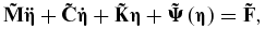
Accurate prediction of large amplitude structural deformations is feasible via non-linear finite element models. However, representation of complex system equations of motion in finite element nodal space requires large degrees of freedom and computational cost that is impractical for design applications(Reference Hollkamp and Gordon44). The governing structural equations of motion for a multiple Degree-Of-Freedom (DOF), geometrically non-linear system with viscous damping can be written as(Reference Rizzi and Muravyov45):
 $$\begin{equation}
{{\bf M\ddot{W}}}\left( t \right) + {{\bf C\dot{W}}}\left( t \right) + {{\bf KW}}\left( t \right) + {{\bf \Psi }}\left( {{{\bf W}}\left( t \right)} \right) = {{\bf F}}\left( t \right)
\end{equation}$$
$$\begin{equation}
{{\bf M\ddot{W}}}\left( t \right) + {{\bf C\dot{W}}}\left( t \right) + {{\bf KW}}\left( t \right) + {{\bf \Psi }}\left( {{{\bf W}}\left( t \right)} \right) = {{\bf F}}\left( t \right)
\end{equation}$$
where M, C and K are the mass, damping, and stiffness matrices, respectively; W is the displacement vector and F represents the force excitation vector. The non-linear forcing term Ψ(W(t)) is a non-linear vector function of W.
An alternative solution approach of the above equation is via transformation to a reduced basis modal coordinate system that dramatically reduces the number of DOFs(Reference McEwan46). The generalised coordinate transformation approach is implemented to obtain a set of coupled modal equations, with reduced DOF:
 $$\begin{equation}
{{\bf W}} = {{\bf \Phi \eta }},
\end{equation}$$
$$\begin{equation}
{{\bf W}} = {{\bf \Phi \eta }},
\end{equation}$$
where  ${{\bm \eta }}$ and Φ are time-dependent vectors of generalised coordinates and a subset of linear eigenvectors (assumed mode shapes vectors), respectively. Via the above transformation, the modal equation results:
 $$\begin{equation}
{{\bf \tilde{M}\ddot{\bm \eta }}} + {{\bf \tilde{C}\dot{\bm \eta }}} + {{\bf \tilde{K}{\bm \eta} }} + {{\bf \tilde{\Psi }}}\left( {{\bm \eta }} \right) = {{\bf \tilde{F}}},
\end{equation}$$
$$\begin{equation}
{{\bf \tilde{M}\ddot{\bm \eta }}} + {{\bf \tilde{C}\dot{\bm \eta }}} + {{\bf \tilde{K}{\bm \eta} }} + {{\bf \tilde{\Psi }}}\left( {{\bm \eta }} \right) = {{\bf \tilde{F}}},
\end{equation}$$
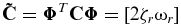
where
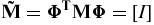 $$\begin{equation}
{{\bf \tilde{M}}} &=& {{{\bf \Phi }}^{{\bf T}}}{{\bf M\Phi }} = \left[ I \right]
\end{equation}$$\\
$$\begin{equation}
{{\bf \tilde{M}}} &=& {{{\bf \Phi }}^{{\bf T}}}{{\bf M\Phi }} = \left[ I \right]
\end{equation}$$\\
 $$\begin{equation}
{{\bf \tilde{C}}} &=& {{{\bf \Phi }}^T}{{\bf C\Phi }} = \left[ {2{\zeta _r}{\omega _r}} \right]
\end{equation}$$\\
$$\begin{equation}
{{\bf \tilde{C}}} &=& {{{\bf \Phi }}^T}{{\bf C\Phi }} = \left[ {2{\zeta _r}{\omega _r}} \right]
\end{equation}$$\\
 $$\begin{equation}
{{\bf \tilde{K}}} &=& {{{\bf \Phi }}^T}{{\bf K\Phi }} = \left[ {\omega _r^2} \right]
\end{equation}$$\\
$$\begin{equation}
{{\bf \tilde{K}}} &=& {{{\bf \Phi }}^T}{{\bf K\Phi }} = \left[ {\omega _r^2} \right]
\end{equation}$$\\
 $$\begin{equation}
{{\bf \tilde{\Psi }}}\left( {{\bm \eta }} \right) &=& {{{\bf \Phi }}^{{\bf T}}}{{\bf \Psi }}\left( {{\bm \eta }} \right)
\end{equation}$$\\
$$\begin{equation}
{{\bf \tilde{\Psi }}}\left( {{\bm \eta }} \right) &=& {{{\bf \Phi }}^{{\bf T}}}{{\bf \Psi }}\left( {{\bm \eta }} \right)
\end{equation}$$\\
 $$\begin{equation}
{\bf \tilde{F}} &=& {{\bf \Phi }^{\bf T}}{{\bf F}} = \left[ {{N_r}} \right],
\end{equation}$$
$$\begin{equation}
{\bf \tilde{F}} &=& {{\bf \Phi }^{\bf T}}{{\bf F}} = \left[ {{N_r}} \right],
\end{equation}$$
 ${{\bf \tilde{\Psi }}}( {{\bm \eta }} )$ brings about the non-linearity and as well as coupling in to the system of equations. However, in absence of large structural displacement, it can be ignored and thus resulting in an uncoupled, linear system of equations as follows:
 $$\begin{equation}
{\ddot{\eta }_r}\left( t \right) + 2{\zeta _r}{\omega _r}{\dot{\eta }_r}\left( t \right) + \omega _r^2{\eta _r}\left( t \right) = {N_r}\left( t \right);\quad r = 1,2,...
\end{equation}$$
$$\begin{equation}
{\ddot{\eta }_r}\left( t \right) + 2{\zeta _r}{\omega _r}{\dot{\eta }_r}\left( t \right) + \omega _r^2{\eta _r}\left( t \right) = {N_r}\left( t \right);\quad r = 1,2,...
\end{equation}$$
 $$\begin{equation}
{N_r}\left( t \right) = \int_D {{\phi _r}\left( P \right)F\left( {P,t} \right)dD\left( P \right),} \quad r = 1,2, \ldots
\end{equation}$$
$$\begin{equation}
{N_r}\left( t \right) = \int_D {{\phi _r}\left( P \right)F\left( {P,t} \right)dD\left( P \right),} \quad r = 1,2, \ldots
\end{equation}$$
where P is an arbitrary point within the domain D.
Equation (9) is subject to the initial generalised displacements and velocities, given below:
 $$\begin{equation}
{\eta _r}\left( 0 \right) &=& \int_D {m\left( P \right){\phi _r}\left( P \right){w_0}\left( P \right)dD\left( P \right),} \quad r = 1,2,...
\end{equation}$$\\
$$\begin{equation}
{\eta _r}\left( 0 \right) &=& \int_D {m\left( P \right){\phi _r}\left( P \right){w_0}\left( P \right)dD\left( P \right),} \quad r = 1,2,...
\end{equation}$$\\
 $$\begin{equation}
{\dot{\eta }_r}\left( 0 \right) &=& \int_D {m\left( P \right){\phi _r}\left( P \right){v_0}\left( P \right)dD\left( P \right),} \quad r = 1,2,...,
\end{equation}$$
$$\begin{equation}
{\dot{\eta }_r}\left( 0 \right) &=& \int_D {m\left( P \right){\phi _r}\left( P \right){v_0}\left( P \right)dD\left( P \right),} \quad r = 1,2,...,
\end{equation}$$
2.2 Inertial force modelling
Due to accelerated motion of the EFW, centrifugal and normal forces are applied to each element. Considering the inherent in-plane tensile strength of the EFW, centrifugal forces are neglected. This is justified as natural frequencies of in-plane modes are normally a few orders of magnitude higher than the natural frequencies of the out-plane ones. Thus, omission of the apparent centrifugal forces is not due to their smaller values, but because of their small effects on structural displacements.
According to Fig. 1, the summation of normal inertial forces applied to an element due to angular acceleration is:
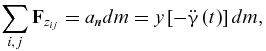 $$\begin{equation}
\sum\limits_{i,j} {{{{\bf F}}_{{z_{ij}}}}} = {a_n}dm = y\left[ { - \ddot{\gamma }\left( t \right)} \right]dm,
\end{equation}$$
$$\begin{equation}
\sum\limits_{i,j} {{{{\bf F}}_{{z_{ij}}}}} = {a_n}dm = y\left[ { - \ddot{\gamma }\left( t \right)} \right]dm,
\end{equation}$$
where Fij is the applied force caused by neighboring elements, an and y are the linear acceleration and position of the mass element dm, respectively, and  $\ddot{\gamma }(t)$ is the angular acceleration of the EFW. Please note that the minus sign in Equation (13) is due to the reference definition of the γ. Thus, according to the Newton's third law of reaction, the applied inertial force from this element to EFW will be:
 $$\begin{equation}
d{F_I} = - y\left[ { - \ddot{\gamma }\left( t \right)} \right]dm = y\ddot{\gamma }\left( t \right)dm
\end{equation}$$
$$\begin{equation}
d{F_I} = - y\left[ { - \ddot{\gamma }\left( t \right)} \right]dm = y\ddot{\gamma }\left( t \right)dm
\end{equation}$$
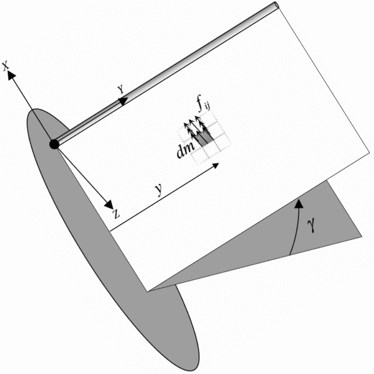
Figure 1. Overall scheme of the inertial forces applied to an element.
Referring to Equation (14), one we can define generalised forces as follows:
 $$\begin{equation}
{N_r}\left( t \right) = \int_D {{\phi _r}d{F_I} = } \int_A {{\phi _r}y\ddot{\gamma }\left( t \right)dm = } \sum\limits_{i,j} {{\phi _{{r_{i,j}}}}{y_{i,j}}\ddot{\gamma }\left( t \right)d{m_{i,j}}} = \ddot{\gamma }\left( t \right){{{\bf \Gamma }}_r},
\end{equation}$$
$$\begin{equation}
{N_r}\left( t \right) = \int_D {{\phi _r}d{F_I} = } \int_A {{\phi _r}y\ddot{\gamma }\left( t \right)dm = } \sum\limits_{i,j} {{\phi _{{r_{i,j}}}}{y_{i,j}}\ddot{\gamma }\left( t \right)d{m_{i,j}}} = \ddot{\gamma }\left( t \right){{{\bf \Gamma }}_r},
\end{equation}$$
where
 $$\begin{equation}
{{{\bf \Gamma }}_r} = \sum\limits_{i,j} {{{{\bf f}}_{{r_{i,j}}}}{y_{i,j}}d{m_{i,j}}}
\end{equation}$$
$$\begin{equation}
{{{\bf \Gamma }}_r} = \sum\limits_{i,j} {{{{\bf f}}_{{r_{i,j}}}}{y_{i,j}}d{m_{i,j}}}
\end{equation}$$
It is realized that, Γr turns out as a structural property that depends on the structure mass distribution and is motion independent. In this sense, it can be referred to as ‘Generalised Inertial Moment’ or GIM.
2.3 Servo motor dynamics
The objective of the servo systems is to control the position of a mechanical system in accordance with a prescribed position. The difference between the input command angular position and the output angular position is the error signal(Reference Ogata47). To model the servo actuator effects on the dynamic response of the EFW, a second order servo dynamics is considered (see Equation (17)) whose transfer function is suggested(Reference Ogata47), with adjustable parameters ζc and ωc defined in the nomenclature.
 $$\begin{equation}
G\left( s \right) = \frac{{\omega _c^2}}{{{s^2} + 2{\zeta _c}{\omega _c}s + \omega _c^2}}
\end{equation}$$
$$\begin{equation}
G\left( s \right) = \frac{{\omega _c^2}}{{{s^2} + 2{\zeta _c}{\omega _c}s + \omega _c^2}}
\end{equation}$$
3.0 ANALYTICAL SOLUTION OF RIGID WING MOTION
In analogy with actual flying EFWs like a bird, it is possible for the flapping motion to stop in a gliding phase of flight. Accordingly, the desired flapping motion can be broken in to a sinusoidal part followed by a command to stop the flapping at a static value. In this respect, the following subsection presents the analytic results of such commands as implemented via a servo actuator.
3.1 Sinusoidal flapping command
Since a part of the EFW motion is sinusoidal, this section will present an analytical solution for the controller output (Equation (17)). As already discussed in Section 2.0, considering a second order transfer function for the controller, will yield,
 $$\begin{equation}
\frac{\gamma }{{{\gamma _{{\rm{Input}}}}}}\left( s \right) = \frac{{\omega _c^2}}{{{s^2} + 2{\zeta _c}{\omega _c}s + \omega _c^2}},
\end{equation}$$
$$\begin{equation}
\frac{\gamma }{{{\gamma _{{\rm{Input}}}}}}\left( s \right) = \frac{{\omega _c^2}}{{{s^2} + 2{\zeta _c}{\omega _c}s + \omega _c^2}},
\end{equation}$$
where
 $$\begin{equation}
{\gamma _{{\rm{Input}}}}\left( t \right) = {\gamma _{{\rm{max}}}}{\rm{sin}}\left( {{\omega _f}t} \right)
\end{equation}$$
$$\begin{equation}
{\gamma _{{\rm{Input}}}}\left( t \right) = {\gamma _{{\rm{max}}}}{\rm{sin}}\left( {{\omega _f}t} \right)
\end{equation}$$
Subsequently, the controller output is determined via Laplace transformations that results in:
 $$\begin{equation}
\gamma \left( s \right) &=& \frac{\gamma }{{{\gamma _{{\rm{Input}}}}}}\left( s \right){\gamma _{{\rm{Input}}}}\left( s \right) = \frac{{{\gamma _{{\rm{max}}}}{\omega _f}\omega _c^2}}{{\left( {{s^2} + 2{\zeta _c}{\omega _c}s + \omega _c^2} \right)\left( {{s^2} + \omega {{_f^{22}}}} \right)}}
\end{equation}$$\\
$$\begin{equation}
\gamma \left( s \right) &=& \frac{\gamma }{{{\gamma _{{\rm{Input}}}}}}\left( s \right){\gamma _{{\rm{Input}}}}\left( s \right) = \frac{{{\gamma _{{\rm{max}}}}{\omega _f}\omega _c^2}}{{\left( {{s^2} + 2{\zeta _c}{\omega _c}s + \omega _c^2} \right)\left( {{s^2} + \omega {{_f^{22}}}} \right)}}
\end{equation}$$\\
 $$\begin{equation}
\gamma \left( t \right) &=& {e^{ - {\zeta _c}{\omega _c}t}}{A_{22}}{\rm{sin}}\left( {{\omega _{{\rm{dc}}}}t + {\phi _{22}}} \right) + {A_{11}}{\rm{sin}}\left( {{\omega _f}t + {\phi _{11}}} \right)
\end{equation}$$
$$\begin{equation}
\gamma \left( t \right) &=& {e^{ - {\zeta _c}{\omega _c}t}}{A_{22}}{\rm{sin}}\left( {{\omega _{{\rm{dc}}}}t + {\phi _{22}}} \right) + {A_{11}}{\rm{sin}}\left( {{\omega _f}t + {\phi _{11}}} \right)
\end{equation}$$
 $$\begin{equation}
{\omega _{{\rm{dc}}}} &=& {\omega _c}\sqrt {1 - \zeta _c^2},
\end{equation}$$\\
$$\begin{equation}
{\omega _{{\rm{dc}}}} &=& {\omega _c}\sqrt {1 - \zeta _c^2},
\end{equation}$$\\
 $$\begin{equation}
{A_{21}}& =& \frac{{{\gamma _{{\rm{max}}}}\frac{{{\omega _f}}}{{{\omega _c}}}}}{{{{\left( {\frac{{{\omega _f}}}{{{\omega _c}}}} \right)}^4} - 2\left( {1 - 2\zeta _c^2} \right){{\left( {\frac{{{\omega _f}}}{{{\omega _c}}}} \right)}^2} + 1}},
\end{equation}$$\\
$$\begin{equation}
{A_{21}}& =& \frac{{{\gamma _{{\rm{max}}}}\frac{{{\omega _f}}}{{{\omega _c}}}}}{{{{\left( {\frac{{{\omega _f}}}{{{\omega _c}}}} \right)}^4} - 2\left( {1 - 2\zeta _c^2} \right){{\left( {\frac{{{\omega _f}}}{{{\omega _c}}}} \right)}^2} + 1}},
\end{equation}$$\\
 $$\begin{equation}
{A_{22}} &=& {A_{21}}\sqrt {{{\left( {\frac{1}{{\sqrt {1 - \zeta _c^2} }}\left[ {{{\left( {\frac{{{\omega _f}}}{{{\omega _c}}}} \right)}^2} - \left( {1 - 2\zeta _c^2} \right)} \right]} \right)}^2} + {{\left( {2{\zeta _c}} \right)}^2}} ,
\end{equation}$$\\
$$\begin{equation}
{A_{22}} &=& {A_{21}}\sqrt {{{\left( {\frac{1}{{\sqrt {1 - \zeta _c^2} }}\left[ {{{\left( {\frac{{{\omega _f}}}{{{\omega _c}}}} \right)}^2} - \left( {1 - 2\zeta _c^2} \right)} \right]} \right)}^2} + {{\left( {2{\zeta _c}} \right)}^2}} ,
\end{equation}$$\\
 $$\begin{equation}
{A_{11}} &=& {A_{21}}\sqrt {{{\left( {{{\left( {\frac{{{\omega _f}}}{{{\omega _c}}}} \right)}^{ - 1}} - \frac{{{\omega _f}}}{{{\omega _c}}}} \right)}^2} + {{\left( {2{\zeta _c}} \right)}^2}} ,
\end{equation}$$\\
$$\begin{equation}
{A_{11}} &=& {A_{21}}\sqrt {{{\left( {{{\left( {\frac{{{\omega _f}}}{{{\omega _c}}}} \right)}^{ - 1}} - \frac{{{\omega _f}}}{{{\omega _c}}}} \right)}^2} + {{\left( {2{\zeta _c}} \right)}^2}} ,
\end{equation}$$\\
 $$\begin{equation}
{\phi _{22}} &=& {\rm{ta}}{{\rm{n}}^{ - 1}}\left( {\frac{{2{\zeta _c}\sqrt {1 - \zeta _c^2} }}{{{{\left( {\frac{{{\omega _f}}}{{{\omega _c}}}} \right)}^2} - \left( {1 - 2\zeta _c^2} \right)}}} \right),
\end{equation}$$\\
$$\begin{equation}
{\phi _{22}} &=& {\rm{ta}}{{\rm{n}}^{ - 1}}\left( {\frac{{2{\zeta _c}\sqrt {1 - \zeta _c^2} }}{{{{\left( {\frac{{{\omega _f}}}{{{\omega _c}}}} \right)}^2} - \left( {1 - 2\zeta _c^2} \right)}}} \right),
\end{equation}$$\\
 $$\begin{equation}
{\phi _{11}} &=& {\rm{ta}}{{\rm{n}}^{ - 1}}\left( { - \frac{{2{\zeta _c}\frac{{{\omega _f}}}{{{\omega _c}}}}}{{1 - {{\left( {\frac{{{\omega _f}}}{{{\omega _c}}}} \right)}^2}}}} \right)
\end{equation}$$
$$\begin{equation}
{\phi _{11}} &=& {\rm{ta}}{{\rm{n}}^{ - 1}}\left( { - \frac{{2{\zeta _c}\frac{{{\omega _f}}}{{{\omega _c}}}}}{{1 - {{\left( {\frac{{{\omega _f}}}{{{\omega _c}}}} \right)}^2}}}} \right)
\end{equation}$$
Noting Equation (21), the controller response (to sinusoidal input) contains a transient fading part plus a time varying portion that can be regarded as a steady forcing on the EFW that is obtained as follows:
 $$\begin{equation}
\begin{array}{@{}l@{}} \mathop {{\rm{lim}}\gamma \left( t \right)}\limits_{t \to \infty } = \mathop {{\rm{lim}}}\limits_{t \to \infty } \left[ {{e^{ - {\zeta _c}{\omega _c}t}}{A_{22}}{\rm{sin}}\left( {{\omega _{{\rm{dc}}}}t + {\phi _{22}}} \right) + {A_{11}}{\rm{sin}}\left( {{\omega _f}t + {\phi _{11}}} \right)} \right]\\ \quad \quad \quad\hspace*{3.5pt} = {A_{11}}{\rm{sin}}\left( {{\omega _f}t + {\phi _{11}}} \right)\\ \quad \quad \quad\hspace*{3.5pt} = {\gamma _{{\rm{max}}}}\frac{{\frac{{{\omega _f}}}{{{\omega _c}}}\sqrt {{{\left( {{{\left( {\frac{{{\omega _f}}}{{{\omega _c}}}} \right)}^{ - 1}} - \frac{{{\omega _f}}}{{{\omega _c}}}} \right)}^2} + {{\left( {2{\zeta _c}} \right)}^2}} }}{{{{\left( {\frac{{{\omega _f}}}{{{\omega _c}}}} \right)}^4} - 2\left( {1 - 2{\zeta _c}^2} \right){{\left( {\frac{{{\omega _f}}}{{{\omega _c}}}} \right)}^2} + 1}}{\rm{sin}}\left( {{\omega _f}t + {\phi _{11}}} \right)\, \end{array}
\end{equation}$$
$$\begin{equation}
\begin{array}{@{}l@{}} \mathop {{\rm{lim}}\gamma \left( t \right)}\limits_{t \to \infty } = \mathop {{\rm{lim}}}\limits_{t \to \infty } \left[ {{e^{ - {\zeta _c}{\omega _c}t}}{A_{22}}{\rm{sin}}\left( {{\omega _{{\rm{dc}}}}t + {\phi _{22}}} \right) + {A_{11}}{\rm{sin}}\left( {{\omega _f}t + {\phi _{11}}} \right)} \right]\\ \quad \quad \quad\hspace*{3.5pt} = {A_{11}}{\rm{sin}}\left( {{\omega _f}t + {\phi _{11}}} \right)\\ \quad \quad \quad\hspace*{3.5pt} = {\gamma _{{\rm{max}}}}\frac{{\frac{{{\omega _f}}}{{{\omega _c}}}\sqrt {{{\left( {{{\left( {\frac{{{\omega _f}}}{{{\omega _c}}}} \right)}^{ - 1}} - \frac{{{\omega _f}}}{{{\omega _c}}}} \right)}^2} + {{\left( {2{\zeta _c}} \right)}^2}} }}{{{{\left( {\frac{{{\omega _f}}}{{{\omega _c}}}} \right)}^4} - 2\left( {1 - 2{\zeta _c}^2} \right){{\left( {\frac{{{\omega _f}}}{{{\omega _c}}}} \right)}^2} + 1}}{\rm{sin}}\left( {{\omega _f}t + {\phi _{11}}} \right)\, \end{array}
\end{equation}$$
Comparing the above analytic controller output with the sinusoidal input (Equation (19)), one can realize the effect of servo dynamics on both amplitude and phase shift of the sinusoidal forcing motion. In other words, for a very fast actuator with a high operating frequency sufficiently greater than EFW flapping frequency, the flapping motion will be close to the commanded value.
 $$\begin{equation}
\mathop {{\rm{lim}}\gamma \left( t \right)}\limits_{t \to \infty ,\frac{{{\omega _f}}}{{{\omega _c}}} \to 0} = {\gamma _{{\rm{max}}}}{\rm{sin}}\left( {{\omega _f}t} \right)
\end{equation}$$
$$\begin{equation}
\mathop {{\rm{lim}}\gamma \left( t \right)}\limits_{t \to \infty ,\frac{{{\omega _f}}}{{{\omega _c}}} \to 0} = {\gamma _{{\rm{max}}}}{\rm{sin}}\left( {{\omega _f}t} \right)
\end{equation}$$
3.2 Stopping command
In this case, it is assumed that the EFW flapping is suddenly commanded to perform a stopping manoeuver towards a fixed flapping angle at ti, such that:
 $$\begin{equation}
{\gamma _{{\rm{Input}}}} = \Delta {\gamma _{{\rm{glide}}}};\quad \Delta {\gamma _{{\rm{glide}}}} = {\gamma _{{\rm{Stop}}}} - \gamma ({t_i}),
\end{equation}$$
$$\begin{equation}
{\gamma _{{\rm{Input}}}} = \Delta {\gamma _{{\rm{glide}}}};\quad \Delta {\gamma _{{\rm{glide}}}} = {\gamma _{{\rm{Stop}}}} - \gamma ({t_i}),
\end{equation}$$
where γ(ti) and γStop are the current and final flapping angles of the EFW for a final glide operation, respectively. Again, via Laplace transformation, one can show the actual commanded result due to the servo dynamic to be as follows:
 $$\begin{equation}
&&\begin{array}{@{}l@{}} \gamma \left( s \right) = \displaystyle\frac{\gamma }{{{\gamma _{{\rm{Stop}}}}}}\left( s \right){\gamma _{{\rm{Stop}}}}\left( s \right)\\ \quad \quad = \displaystyle\frac{{\Delta {\gamma _{{\rm{glide}}}}\omega _c^2}}{{s\left( {{s^2} + 2{\zeta _c}{\omega _c}s + \omega _c^2} \right)}} \end{array},
\end{equation}$$\\
$$\begin{equation}
&&\begin{array}{@{}l@{}} \gamma \left( s \right) = \displaystyle\frac{\gamma }{{{\gamma _{{\rm{Stop}}}}}}\left( s \right){\gamma _{{\rm{Stop}}}}\left( s \right)\\ \quad \quad = \displaystyle\frac{{\Delta {\gamma _{{\rm{glide}}}}\omega _c^2}}{{s\left( {{s^2} + 2{\zeta _c}{\omega _c}s + \omega _c^2} \right)}} \end{array},
\end{equation}$$\\
 $$\begin{equation}
&&\gamma \left( t \right) = {\gamma _{{\rm{Stop}}}} - {e^{ - {\zeta _c}{\omega _c}t}}{B_{11}}{\rm{sin}}\left( {{\omega _{{\rm{dc}}}}t + {\psi _{11}}} \right),
\end{equation}$$
$$\begin{equation}
&&\gamma \left( t \right) = {\gamma _{{\rm{Stop}}}} - {e^{ - {\zeta _c}{\omega _c}t}}{B_{11}}{\rm{sin}}\left( {{\omega _{{\rm{dc}}}}t + {\psi _{11}}} \right),
\end{equation}$$
 $$\begin{equation}
{B_{11}} = \frac{{\Delta {\gamma _{{\rm{glide}}}}}}{{\sqrt {1 - \zeta _c^2} }} ;\quad {\psi _{11}} = {\rm{ta}}{{\rm{n}}^{ - 1}}\left( {\frac{{\sqrt {1 - \zeta _c^2} }}{{{\zeta _c}}}} \right)
\end{equation}$$
$$\begin{equation}
{B_{11}} = \frac{{\Delta {\gamma _{{\rm{glide}}}}}}{{\sqrt {1 - \zeta _c^2} }} ;\quad {\psi _{11}} = {\rm{ta}}{{\rm{n}}^{ - 1}}\left( {\frac{{\sqrt {1 - \zeta _c^2} }}{{{\zeta _c}}}} \right)
\end{equation}$$
Additionally, similar to Section 3.1, one can observe that limiting desired value is eventually reached after some elapsed time.
 $$\begin{equation}
\mathop {{\rm{lim}}\gamma \left( t \right)}\limits_{t \to \infty } = {\gamma _{{\rm{Stop}}}}
\end{equation}$$
$$\begin{equation}
\mathop {{\rm{lim}}\gamma \left( t \right)}\limits_{t \to \infty } = {\gamma _{{\rm{Stop}}}}
\end{equation}$$
It is realized from Equations (32) and (34) that the controller dynamics does not have any effect on the final steady result and the actuator will finally place the EFW at the desired flapping position. The resulting graphical summary of the above cases are shown in Fig. 4 as a part of the simulation scenario presented in Section 5.0.
4.0 ANALYTICAL SOLUTION OF EFW
In this section, the analytical solution for the structural behaviour of the EFW is presented. The analytical solution is developed in two parts that includes response to a pure flapping command as well as the EFW response to a flap angle command.
4.1 Sinusoidal flapping response
As a requirement for the solution of the governing structural equations, Equations (9) and (15),  $\ddot{\gamma }(t)$ is required to calculate the generalised forces. In this respect, one can obtain the flapping angular acceleration via Equation (21), to be:
 $$\begin{equation}
\ddot{\gamma }\left( t \right) = {e^{ - {\zeta _c}{\omega _c}t}}\left[ {{{\skew5\hat{A}}_{22}}{\rm{sin}}\left( {{\omega _{{\rm{dc}}}}t + {{\hat{\phi }}_{22}}} \right)} \right] + {\skew5\hat{A}_{11}}\,{\rm{sin}}\left( {{\omega _f}t + {\phi _{11}}} \right),
\end{equation}$$
$$\begin{equation}
\ddot{\gamma }\left( t \right) = {e^{ - {\zeta _c}{\omega _c}t}}\left[ {{{\skew5\hat{A}}_{22}}{\rm{sin}}\left( {{\omega _{{\rm{dc}}}}t + {{\hat{\phi }}_{22}}} \right)} \right] + {\skew5\hat{A}_{11}}\,{\rm{sin}}\left( {{\omega _f}t + {\phi _{11}}} \right),
\end{equation}$$
where
 $$\begin{equation}
{\skew5\hat{A}_{22}} = - {A_{22}}\omega _c^2;\;{\skew5\hat{A}_{11}} = - {A_{11}}\omega _f^2 ;\quad {\hat{\phi }_{22}} = {\phi _{22}} + {\rm{ta}}{{\rm{n}}^{ - 1}}\left( {\frac{{2{\zeta _c}\sqrt {1 - \zeta _c^2} }}{{1 - 2\zeta _c^2}}} \right)
\end{equation}$$
$$\begin{equation}
{\skew5\hat{A}_{22}} = - {A_{22}}\omega _c^2;\;{\skew5\hat{A}_{11}} = - {A_{11}}\omega _f^2 ;\quad {\hat{\phi }_{22}} = {\phi _{22}} + {\rm{ta}}{{\rm{n}}^{ - 1}}\left( {\frac{{2{\zeta _c}\sqrt {1 - \zeta _c^2} }}{{1 - 2\zeta _c^2}}} \right)
\end{equation}$$
Substituting Equation (35) in Equation (15) and Equation (9) yields the desired Ordinary Differential Equation (ODE) for dynamic behaviour of the EFW under sinusoidal actuation.
 $$\begin{equation}
\begin{array}{@{}l@{}} {{\ddot{\eta }}_r}\left( t \right) + 2{\zeta _r}{\omega _r}{{\dot{\eta }}_r}\left( t \right) + \omega _r^2{\eta _r}\left( t \right) = {{\skew5\hat{A}}_{22}}{{{\bf \Gamma }}_r}{e^{ - {\zeta _c}{\omega _c}t}}{\rm{sin}}\left( {{\omega _{{\rm{dc}}}}t + {{\hat{\phi }}_{22}}} \right) + {{{\bf \Gamma }}_r}{{\skew5\hat{A}}_{11}}{\rm{sin}}\left( {{\omega _f}t + {\phi _{11}}} \right)\\ \quad {\eta _r}\left( 0 \right) = {\eta _{r0}};\quad {{\dot{\eta }}_r}\left( 0 \right) = {{\dot{\eta }}_{r0}} \end{array}
\end{equation}$$
$$\begin{equation}
\begin{array}{@{}l@{}} {{\ddot{\eta }}_r}\left( t \right) + 2{\zeta _r}{\omega _r}{{\dot{\eta }}_r}\left( t \right) + \omega _r^2{\eta _r}\left( t \right) = {{\skew5\hat{A}}_{22}}{{{\bf \Gamma }}_r}{e^{ - {\zeta _c}{\omega _c}t}}{\rm{sin}}\left( {{\omega _{{\rm{dc}}}}t + {{\hat{\phi }}_{22}}} \right) + {{{\bf \Gamma }}_r}{{\skew5\hat{A}}_{11}}{\rm{sin}}\left( {{\omega _f}t + {\phi _{11}}} \right)\\ \quad {\eta _r}\left( 0 \right) = {\eta _{r0}};\quad {{\dot{\eta }}_r}\left( 0 \right) = {{\dot{\eta }}_{r0}} \end{array}
\end{equation}$$
The analytical solution of this ODE is determined using the specified initial conditions.
 $$\begin{eqnarray}
{\eta _r}\left( t \right) &=& {A_1}\;{\rm{sin}}\left( {{\omega _f}t + {\phi _1}} \right) + {e^{ - {\zeta _c}{\omega _c}t}}{A_2}\;{\rm{sin}}\left( {{\omega _{{\rm{dc}}}}t + {\phi _2}} \right)\nonumber\\
&& +\, {e^{ - {\zeta _r}{\omega _r}t}}{A_3}\;{\rm{sin}}\left( {{\omega _{dr}}t + {\phi _3}} \right),\quad r = 1,2, \ldots ,
\end{eqnarray}$$
$$\begin{eqnarray}
{\eta _r}\left( t \right) &=& {A_1}\;{\rm{sin}}\left( {{\omega _f}t + {\phi _1}} \right) + {e^{ - {\zeta _c}{\omega _c}t}}{A_2}\;{\rm{sin}}\left( {{\omega _{{\rm{dc}}}}t + {\phi _2}} \right)\nonumber\\
&& +\, {e^{ - {\zeta _r}{\omega _r}t}}{A_3}\;{\rm{sin}}\left( {{\omega _{dr}}t + {\phi _3}} \right),\quad r = 1,2, \ldots ,
\end{eqnarray}$$
where
 $$\begin{equation}
{\omega _{dr}} &=& {\omega _r}\sqrt {1 - \zeta _r^2} ,
\end{equation}$$\\
$$\begin{equation}
{\omega _{dr}} &=& {\omega _r}\sqrt {1 - \zeta _r^2} ,
\end{equation}$$\\
 $$\begin{equation}
{A_3} &=& \frac{{{\eta _{r0}} - {A_2}\;{\rm{sin}}\left( {{\phi _2}} \right) - {A_1}\,{\rm{sin}}\left( {{\phi _1}} \right)}}{{{\rm{sin}}\left( {{\phi _3}} \right)}},
\end{equation}$$\\
$$\begin{equation}
{A_3} &=& \frac{{{\eta _{r0}} - {A_2}\;{\rm{sin}}\left( {{\phi _2}} \right) - {A_1}\,{\rm{sin}}\left( {{\phi _1}} \right)}}{{{\rm{sin}}\left( {{\phi _3}} \right)}},
\end{equation}$$\\
 $$\begin{equation}
{\phi _3} &=& {\rm{ta}}{{\rm{n}}^{ - 1}}
{\fontsize{11}{13}\selectfont{\begin{array}{l}\left\{ {\frac{{\frac{{{\omega _r}}}{{{\omega _c}}}\sqrt {1 - {\zeta _r}^2} \left[ {{\eta _{r0}} - {A_2}\;{\rm{sin}}\left( {{\phi _2}} \right) - {A_1}\;{\rm{sin}}\left( {{\phi _1}} \right)} \right]}}{{\frac{{{{\dot{\eta }}_{r0}}}}{{{\omega _c}}} - {A_1}\frac{{{\omega _f}}}{{{\omega _c}}}{\rm{cos}}\left( {{\phi _1}} \right) + {\zeta _c}{A_2}\;{\rm{sin}}\left( {{\phi _2}} \right) - \sqrt {1 - \zeta _c^2} {A_2}\;{\rm{cos}}\left( {{\phi _2}} \right) + {\zeta _r}\frac{{{\omega _r}}}{{{\omega _c}}}\left[ {{\eta _{r0}} - {A_2}\;{\rm{sin}}\left( {{\phi _2}} \right) - {A_1}\;{\rm{sin}}\left( {{\phi _1}} \right)} \right]}}} \right\},\end{array}}}\nonumber\\
\end{equation}$$\\
$$\begin{equation}
{\phi _3} &=& {\rm{ta}}{{\rm{n}}^{ - 1}}
{\fontsize{11}{13}\selectfont{\begin{array}{l}\left\{ {\frac{{\frac{{{\omega _r}}}{{{\omega _c}}}\sqrt {1 - {\zeta _r}^2} \left[ {{\eta _{r0}} - {A_2}\;{\rm{sin}}\left( {{\phi _2}} \right) - {A_1}\;{\rm{sin}}\left( {{\phi _1}} \right)} \right]}}{{\frac{{{{\dot{\eta }}_{r0}}}}{{{\omega _c}}} - {A_1}\frac{{{\omega _f}}}{{{\omega _c}}}{\rm{cos}}\left( {{\phi _1}} \right) + {\zeta _c}{A_2}\;{\rm{sin}}\left( {{\phi _2}} \right) - \sqrt {1 - \zeta _c^2} {A_2}\;{\rm{cos}}\left( {{\phi _2}} \right) + {\zeta _r}\frac{{{\omega _r}}}{{{\omega _c}}}\left[ {{\eta _{r0}} - {A_2}\;{\rm{sin}}\left( {{\phi _2}} \right) - {A_1}\;{\rm{sin}}\left( {{\phi _1}} \right)} \right]}}} \right\},\end{array}}}\nonumber\\
\end{equation}$$\\
 $$\begin{equation}
{A_2} &=& - \frac{{{\Gamma _r}{A_{22}}}}{{\sqrt {{{\left[ {{{\left( {\frac{{{\omega _r}}}{{{\omega _c}}}} \right)}^2} - \left( {1 - 2\zeta _c^2} \right) - 2{\xi _r}{\zeta _c}\left( {\frac{{{\omega _r}}}{{{\omega _c}}}} \right)} \right]}^2} + {{\left[ {2{\zeta _r}\left( {\frac{{{\omega _r}}}{{{\omega _c}}}} \right)\sqrt {1 - \zeta _c^2} - 2{\zeta _c}\sqrt {1 - \zeta _c^2} } \right]}^2}} }},\nonumber\\
\end{equation}$$\\
$$\begin{equation}
{A_2} &=& - \frac{{{\Gamma _r}{A_{22}}}}{{\sqrt {{{\left[ {{{\left( {\frac{{{\omega _r}}}{{{\omega _c}}}} \right)}^2} - \left( {1 - 2\zeta _c^2} \right) - 2{\xi _r}{\zeta _c}\left( {\frac{{{\omega _r}}}{{{\omega _c}}}} \right)} \right]}^2} + {{\left[ {2{\zeta _r}\left( {\frac{{{\omega _r}}}{{{\omega _c}}}} \right)\sqrt {1 - \zeta _c^2} - 2{\zeta _c}\sqrt {1 - \zeta _c^2} } \right]}^2}} }},\nonumber\\
\end{equation}$$\\
 $$\begin{equation}
{A_1} &=& \frac{{ - {\Gamma _r}{{\left( {\frac{{{\omega _f}}}{{{\omega _r}}}} \right)}^2}{A_{11}}}}{{\sqrt {{{\left( {1 - {{\left( {\frac{{{\omega _f}}}{{{\omega _r}}}} \right)}^2}} \right)}^2} + {{\left( {2{\zeta _r}\left( {\frac{{{\omega _f}}}{{{\omega _r}}}} \right)} \right)}^2}} }},
\end{equation}$$\\
$$\begin{equation}
{A_1} &=& \frac{{ - {\Gamma _r}{{\left( {\frac{{{\omega _f}}}{{{\omega _r}}}} \right)}^2}{A_{11}}}}{{\sqrt {{{\left( {1 - {{\left( {\frac{{{\omega _f}}}{{{\omega _r}}}} \right)}^2}} \right)}^2} + {{\left( {2{\zeta _r}\left( {\frac{{{\omega _f}}}{{{\omega _r}}}} \right)} \right)}^2}} }},
\end{equation}$$\\
 $$\begin{equation}
{\phi _2}& =& {\rm{ta}}{{\rm{n}}^{ - 1}}
{\fontsize{11}{13}\selectfont{\begin{array}{l}\left( {\frac{{2{\zeta _c}\left( {1 - \zeta _c^2} \right)}}{{{{\left( {\frac{{{\omega _f}}}{{{\omega _c}}}} \right)}^2} - \left( {1 - 2\zeta _c^2} \right)}}} \right)\! +\! {\rm{ta}}{{\rm{n}}^{ - 1}}\left( {\frac{{2{\zeta _c}\sqrt {1 - \zeta _c^2} }}{{1 - 2\zeta _c^2}}} \right)\! -\! {\rm{ta}}{{\rm{n}}^{ - 1}}\left( {\frac{{2{\zeta _r}\frac{{{\omega _r}}}{{{\omega _c}}}\sqrt {1 - \zeta _c^2} - 2{\zeta _c}\sqrt {1 - \zeta _c^2} }}{{{{\left( {\frac{{{\omega _r}}}{{{\omega _c}}}} \right)}^2} - 2{\zeta _r}{\zeta _c}\frac{{{\omega _r}}}{{{\omega _c}}} - \left( {1 - 2\zeta _c^2} \right)}}} \right),\end{array}}}\nonumber\\
\end{equation}$$\\
$$\begin{equation}
{\phi _2}& =& {\rm{ta}}{{\rm{n}}^{ - 1}}
{\fontsize{11}{13}\selectfont{\begin{array}{l}\left( {\frac{{2{\zeta _c}\left( {1 - \zeta _c^2} \right)}}{{{{\left( {\frac{{{\omega _f}}}{{{\omega _c}}}} \right)}^2} - \left( {1 - 2\zeta _c^2} \right)}}} \right)\! +\! {\rm{ta}}{{\rm{n}}^{ - 1}}\left( {\frac{{2{\zeta _c}\sqrt {1 - \zeta _c^2} }}{{1 - 2\zeta _c^2}}} \right)\! -\! {\rm{ta}}{{\rm{n}}^{ - 1}}\left( {\frac{{2{\zeta _r}\frac{{{\omega _r}}}{{{\omega _c}}}\sqrt {1 - \zeta _c^2} - 2{\zeta _c}\sqrt {1 - \zeta _c^2} }}{{{{\left( {\frac{{{\omega _r}}}{{{\omega _c}}}} \right)}^2} - 2{\zeta _r}{\zeta _c}\frac{{{\omega _r}}}{{{\omega _c}}} - \left( {1 - 2\zeta _c^2} \right)}}} \right),\end{array}}}\nonumber\\
\end{equation}$$\\
 $$\begin{equation}
{\phi _1} &=& {\rm{ta}}{{\rm{n}}^{ - 1}}\left( { - \frac{{2{\zeta _c}\frac{{{\omega _f}}}{{{\omega _c}}}}}{{1 - {{\left( {\frac{{{\omega _f}}}{{{\omega _c}}}} \right)}^2}}}} \right) - {\rm{ta}}{{\rm{n}}^{ - 1}}\left( {\frac{{2{\xi _r}\frac{{{\omega _f}}}{{{\omega _r}}}}}{{1 - {{\left( {\frac{{{\omega _f}}}{{{\omega _r}}}} \right)}^2}}}} \right)
\end{equation}$$
$$\begin{equation}
{\phi _1} &=& {\rm{ta}}{{\rm{n}}^{ - 1}}\left( { - \frac{{2{\zeta _c}\frac{{{\omega _f}}}{{{\omega _c}}}}}{{1 - {{\left( {\frac{{{\omega _f}}}{{{\omega _c}}}} \right)}^2}}}} \right) - {\rm{ta}}{{\rm{n}}^{ - 1}}\left( {\frac{{2{\xi _r}\frac{{{\omega _f}}}{{{\omega _r}}}}}{{1 - {{\left( {\frac{{{\omega _f}}}{{{\omega _r}}}} \right)}^2}}}} \right)
\end{equation}$$
The resulting analytical solution (Equations (38) to (45)) indicates that larger natural frequencies of the structural mode shapes tend to have no significant effect on the EFW dynamic behaviour, as shown below:
 $$\begin{equation}
\mathop {{\rm{lim}}}\limits_{{\omega _r} \to \infty } {\eta _r}\left( t \right) = 0
\end{equation}$$
$$\begin{equation}
\mathop {{\rm{lim}}}\limits_{{\omega _r} \to \infty } {\eta _r}\left( t \right) = 0
\end{equation}$$
In addition, it is also seen that at Structure-Actuator Frequency Ratio (SAFR) close to one, i.e.  ${{{\omega _r}}
/ {{\omega _c}}} \to 1$, existence of the actuation damping, ζc effectively bounds A 2 (Equation (42)) that in turn prevents the second term of the EFW dynamic response (Equation (38)) from growing. To check the conditions for other resonance behaviours, other coefficients will also be examined. In this respect, when there is insignificant or zero structural damping, ζr → 0, A 1 and consequently A 3 tend towards infinity at Structure-Flapping Frequency Ratio (SFFR) close to one i.e.
${{{\omega _r}}
/ {{\omega _c}}} \to 1$, existence of the actuation damping, ζc effectively bounds A 2 (Equation (42)) that in turn prevents the second term of the EFW dynamic response (Equation (38)) from growing. To check the conditions for other resonance behaviours, other coefficients will also be examined. In this respect, when there is insignificant or zero structural damping, ζr → 0, A 1 and consequently A 3 tend towards infinity at Structure-Flapping Frequency Ratio (SFFR) close to one i.e.  ${{{\omega _f}}
/ {{\omega _r}}} \to 1$. Figure 2 shows the variation of A 1 for two different values of ζr as a function of SAFR and SFFR. According to this figure, it is seen that A 1 achieves its pick value for resonance conditions of both frequency ratios i.e.
${{{\omega _f}}
/ {{\omega _r}}} \to 1$. Figure 2 shows the variation of A 1 for two different values of ζr as a function of SAFR and SFFR. According to this figure, it is seen that A 1 achieves its pick value for resonance conditions of both frequency ratios i.e.  ${{{\omega _f}}
/ {{\omega _r}}} \to 1\;{\rm{and}}\;{{{\omega _r}}
/ {{\omega _c}}} \to 1$. Finally, Fig. 3 shows the variation of A 1 at resonance conditions as a function of the EFW structural damping, ζr.
${{{\omega _f}}
/ {{\omega _r}}} \to 1\;{\rm{and}}\;{{{\omega _r}}
/ {{\omega _c}}} \to 1$. Finally, Fig. 3 shows the variation of A 1 at resonance conditions as a function of the EFW structural damping, ζr.
Figure 2. The variation of A 1 values versus frequency ratios at (a) ζr = 0.07 and (b) ζr = 0.00001.

Figure 3. The variation of A 1 values versus structural damping ratio at  ${{{\omega _r}}
/ {{\omega _c}}} = {{{\omega _f}}
/ {{\omega _c}}} = 1$.
${{{\omega _r}}
/ {{\omega _c}}} = {{{\omega _f}}
/ {{\omega _c}}} = 1$.
4.2 Response to flap angle (glide) command
In analogy with the sinusoidal forcing discussed in Section 4.1, flapping acceleration actuator output is again required to calculate generalised forces. Using Equation (32), it can be shown that:
 $$\begin{equation}
\ddot{\gamma }\left( t \right) = {\hat{B}_{11}}{e^{ - {\zeta _c}{\omega _c}t}}{\rm{sin}}\left( {{\omega _{{\rm{dc}}}}t + {{\hat{\psi }}_{11}}} \right),
\end{equation}$$
$$\begin{equation}
\ddot{\gamma }\left( t \right) = {\hat{B}_{11}}{e^{ - {\zeta _c}{\omega _c}t}}{\rm{sin}}\left( {{\omega _{{\rm{dc}}}}t + {{\hat{\psi }}_{11}}} \right),
\end{equation}$$
where
 $$\begin{equation}
{\hat{B}_{11}} = {B_{11}}\omega _c^2 ;\quad {\hat{\psi }_{11}} = {\psi _{11}} + {\rm{ta}}{{\rm{n}}^{ - 1}}\left( {\frac{{2{\zeta _c}\sqrt {1 - \zeta _c^2} }}{{1 - 2\zeta _c^2}}} \right)
\end{equation}$$
$$\begin{equation}
{\hat{B}_{11}} = {B_{11}}\omega _c^2 ;\quad {\hat{\psi }_{11}} = {\psi _{11}} + {\rm{ta}}{{\rm{n}}^{ - 1}}\left( {\frac{{2{\zeta _c}\sqrt {1 - \zeta _c^2} }}{{1 - 2\zeta _c^2}}} \right)
\end{equation}$$
Substituting Equation (47) in Equation (15) and next in Equation (9), the ODE governing EFW structural dynamic response as well as its solution are analytically computed.
 $$\begin{eqnarray}
&&{\ddot{\eta }_r}\left( t \right) + 2{\zeta _r}{\omega _r}{\dot{\eta }_r}\left( t \right) + \omega _r^2{\eta _r}\left( t \right) = {\Gamma _r}{\hat{B}_{11}}{e^{ - {\zeta _c}{\omega _c}t}}{\rm{sin}}\left( {{\omega _{dc}}t + {{\hat{\psi }}_{11}}} \right);\nonumber\\
&&\quad {\eta _r}\left( 0 \right) = {\eta _{r0}};\quad {\dot{\eta }_r}\left( 0 \right) = {\dot{\eta }_{r0}},
\end{eqnarray}$$\\
$$\begin{eqnarray}
&&{\ddot{\eta }_r}\left( t \right) + 2{\zeta _r}{\omega _r}{\dot{\eta }_r}\left( t \right) + \omega _r^2{\eta _r}\left( t \right) = {\Gamma _r}{\hat{B}_{11}}{e^{ - {\zeta _c}{\omega _c}t}}{\rm{sin}}\left( {{\omega _{dc}}t + {{\hat{\psi }}_{11}}} \right);\nonumber\\
&&\quad {\eta _r}\left( 0 \right) = {\eta _{r0}};\quad {\dot{\eta }_r}\left( 0 \right) = {\dot{\eta }_{r0}},
\end{eqnarray}$$\\
 $$\begin{equation}
{\eta _r}\left( t \right) = {e^{ - {\zeta _r}{\omega _r}t}}{B_2}\;{\rm{sin}}\left( {{\omega _{dr}}t + {\psi _2}} \right) + {B_1}{e^{ - {\zeta _c}{\omega _c}t}}\;{\rm{sin}}\left( {{\omega _{{\rm{dc}}}}t + {\psi _1}} \right),\quad r = 1,2, \ldots ,
\end{equation}$$
$$\begin{equation}
{\eta _r}\left( t \right) = {e^{ - {\zeta _r}{\omega _r}t}}{B_2}\;{\rm{sin}}\left( {{\omega _{dr}}t + {\psi _2}} \right) + {B_1}{e^{ - {\zeta _c}{\omega _c}t}}\;{\rm{sin}}\left( {{\omega _{{\rm{dc}}}}t + {\psi _1}} \right),\quad r = 1,2, \ldots ,
\end{equation}$$
where
 $$\begin{equation}
{\psi _2} &=& {\rm{ta}}{{\rm{n}}^{ - 1}}\left\{ {\frac{{\frac{{{\omega _r}}}{{{\omega _c}}}\sqrt {1 - \zeta _r^2} \left( {{\eta _{r0}} - {B_1}\;{\rm{sin}}\left( {{\psi _1}} \right)} \right)}}{{\frac{{{{\dot{\eta }}_{r0}}}}{{{\omega _c}}} - {B_1}\sqrt {1 - \zeta _c^2} \,{\rm{cos}}\left( {{\psi _1}} \right) + {\zeta _c}{B_1}\,{\rm{sin}}\left( {{\psi _1}} \right) + {\zeta _r}\frac{{{\omega _r}}}{{{\omega _c}}}\left( {{\eta _{r0}} - {B_1}\;{\rm{sin}}\left( {{\psi _1}} \right)} \right)}}} \right\},\nonumber\\
\end{equation}$$\\
$$\begin{equation}
{\psi _2} &=& {\rm{ta}}{{\rm{n}}^{ - 1}}\left\{ {\frac{{\frac{{{\omega _r}}}{{{\omega _c}}}\sqrt {1 - \zeta _r^2} \left( {{\eta _{r0}} - {B_1}\;{\rm{sin}}\left( {{\psi _1}} \right)} \right)}}{{\frac{{{{\dot{\eta }}_{r0}}}}{{{\omega _c}}} - {B_1}\sqrt {1 - \zeta _c^2} \,{\rm{cos}}\left( {{\psi _1}} \right) + {\zeta _c}{B_1}\,{\rm{sin}}\left( {{\psi _1}} \right) + {\zeta _r}\frac{{{\omega _r}}}{{{\omega _c}}}\left( {{\eta _{r0}} - {B_1}\;{\rm{sin}}\left( {{\psi _1}} \right)} \right)}}} \right\},\nonumber\\
\end{equation}$$\\
 $$\begin{equation}
{B_2} &=& \frac{{{\eta _{r0}} - {B_1}\;{\rm{sin}}\left( {{\psi _1}} \right)}}{{{\rm{sin}}\left( {{\psi _2}} \right)}},
\end{equation}$$\\
$$\begin{equation}
{B_2} &=& \frac{{{\eta _{r0}} - {B_1}\;{\rm{sin}}\left( {{\psi _1}} \right)}}{{{\rm{sin}}\left( {{\psi _2}} \right)}},
\end{equation}$$\\
 $$\begin{equation}
{B_1} &=& \frac{{\frac{{{\Gamma _r}{\gamma _{{\rm{glide}}}}}}{{\sqrt {1 - \zeta _c^2} }}}}{{\sqrt {{{\left[ {2\left( {\frac{{{\omega _r}}}{{{\omega _c}}}} \right){\zeta _r}\sqrt {1 - \zeta _c^2} - 2{\zeta _c}\sqrt {1 - \zeta _c^2} } \right]}^2} + {{\left[ {{{\left( {\frac{{{\omega _r}}}{{{\omega _c}}}} \right)}^2} - \left( {1 - 2\zeta _c^2} \right) - 2\left( {\frac{{{\omega _r}}}{{{\omega _c}}}} \right){\zeta _r}{\zeta _c}} \right]}^2}} }} \nonumber\\
\end{equation}$$ \\
$$\begin{equation}
{B_1} &=& \frac{{\frac{{{\Gamma _r}{\gamma _{{\rm{glide}}}}}}{{\sqrt {1 - \zeta _c^2} }}}}{{\sqrt {{{\left[ {2\left( {\frac{{{\omega _r}}}{{{\omega _c}}}} \right){\zeta _r}\sqrt {1 - \zeta _c^2} - 2{\zeta _c}\sqrt {1 - \zeta _c^2} } \right]}^2} + {{\left[ {{{\left( {\frac{{{\omega _r}}}{{{\omega _c}}}} \right)}^2} - \left( {1 - 2\zeta _c^2} \right) - 2\left( {\frac{{{\omega _r}}}{{{\omega _c}}}} \right){\zeta _r}{\zeta _c}} \right]}^2}} }} \nonumber\\
\end{equation}$$ \\
 $$\begin{equation}
{\psi _1} &=& {\rm{ta}}{{\rm{n}}^{ - 1}}
{\fontsize{12}{14}\selectfont{\begin{array}{l}\left( {\frac{{\sqrt {1 - \zeta _c^2} }}{{{\zeta _c}}}} \right) + {\rm{ta}}{{\rm{n}}^{ - 1}}\left( {\frac{{2{\zeta _c}\sqrt {1 - \zeta _c^2} }}{{1 - 2\zeta _c^2}}} \right) - {\rm{ta}}{{\rm{n}}^{ - 1}}\left( {\frac{{2\left( {\frac{{{\omega _r}}}{{{\omega _c}}}} \right){\zeta _r}\sqrt {1 - \zeta _c^2} - 2{\zeta _c}\sqrt {1 - \zeta _c^2} }}{{{{\left( {\frac{{{\omega _r}}}{{{\omega _c}}}} \right)}^2} - \left( {1 - 2\zeta _c^2} \right) - 2\left( {\frac{{{\omega _r}}}{{{\omega _c}}}} \right){\zeta _r}{\zeta _c}}}} \right)\end{array}}}\nonumber\\
\end{equation}$$
$$\begin{equation}
{\psi _1} &=& {\rm{ta}}{{\rm{n}}^{ - 1}}
{\fontsize{12}{14}\selectfont{\begin{array}{l}\left( {\frac{{\sqrt {1 - \zeta _c^2} }}{{{\zeta _c}}}} \right) + {\rm{ta}}{{\rm{n}}^{ - 1}}\left( {\frac{{2{\zeta _c}\sqrt {1 - \zeta _c^2} }}{{1 - 2\zeta _c^2}}} \right) - {\rm{ta}}{{\rm{n}}^{ - 1}}\left( {\frac{{2\left( {\frac{{{\omega _r}}}{{{\omega _c}}}} \right){\zeta _r}\sqrt {1 - \zeta _c^2} - 2{\zeta _c}\sqrt {1 - \zeta _c^2} }}{{{{\left( {\frac{{{\omega _r}}}{{{\omega _c}}}} \right)}^2} - \left( {1 - 2\zeta _c^2} \right) - 2\left( {\frac{{{\omega _r}}}{{{\omega _c}}}} \right){\zeta _r}{\zeta _c}}}} \right)\end{array}}}\nonumber\\
\end{equation}$$
The result indicates that higher structural modes have insignificant effect on the final static position of the EFW, pending higher modes are not initially excited, or in other words:
 $$\begin{equation}
\mathop {{\rm{lim}}}\limits_{{\omega _r} \to \infty } {\eta _r}\left( t \right) = 0
\end{equation}$$
$$\begin{equation}
\mathop {{\rm{lim}}}\limits_{{\omega _r} \to \infty } {\eta _r}\left( t \right) = 0
\end{equation}$$
5.0 CASE STUDY
To better understand the EFW dynamic behaviour subsequent to commanded flapping, a case study is performed in this section where the commanded flapping consists of two parts whose analytical solutions have already been developed. It needs to be mentioned that the EFW natural frequencies and mode shapes are required for dynamic response analysis and calculated via FEM.
5.1 Flapping scenario
To analyse the EFW structural response, a flapping scenario is considered where the actuator initially commands a sinusoidal behaviour (from rest) to be stopped at a certain glide angle. The commanded flapping angle as well as the corresponding servo output are shown in Fig. 4. Subsequently, the EFW corresponding analytical solutions (Equations (38) and (50)) are determined based on the following initial conditions:
 $$\begin{equation}
&&\left\{ \begin{array}{@{}l@{}} {\eta _{{r_{{\rm{phase}}\,\,{\rm{I}}}}}}\left( {t = 0} \right) = 0\\ {{\dot{\eta }}_{{r_{{\rm{phase}}\,\,{\rm{I}}}}}}\left( {t = 0} \right) = 0 \end{array} \right.,
\end{equation}$$\\
$$\begin{equation}
&&\left\{ \begin{array}{@{}l@{}} {\eta _{{r_{{\rm{phase}}\,\,{\rm{I}}}}}}\left( {t = 0} \right) = 0\\ {{\dot{\eta }}_{{r_{{\rm{phase}}\,\,{\rm{I}}}}}}\left( {t = 0} \right) = 0 \end{array} \right.,
\end{equation}$$\\
 $$\begin{equation}
&&\left\{ \begin{array}{@{}l@{}} {\eta _{{r_{{\rm{phase}}\;\,{\rm{II}}}}}}\left( {t = {t_{{\rm{glide}}}}} \right) = {\eta _{{r_{{\rm{phase}}\,\,{\rm{I}}}}}}\left( {t = {t_{{\rm{glide}}}}} \right)\\ {{\dot{\eta }}_{{r_{{\rm{phase}}\;\,{\rm{II}}}}}}\left( {t = {t_{{\rm{glide}}}}} \right) = {{\dot{\eta }}_{{r_{{\rm{phase}}\,\,{\rm{I}}}}}}\left( {t = {t_{{\rm{glide}}}}} \right) \end{array} \right.
\end{equation}$$
$$\begin{equation}
&&\left\{ \begin{array}{@{}l@{}} {\eta _{{r_{{\rm{phase}}\;\,{\rm{II}}}}}}\left( {t = {t_{{\rm{glide}}}}} \right) = {\eta _{{r_{{\rm{phase}}\,\,{\rm{I}}}}}}\left( {t = {t_{{\rm{glide}}}}} \right)\\ {{\dot{\eta }}_{{r_{{\rm{phase}}\;\,{\rm{II}}}}}}\left( {t = {t_{{\rm{glide}}}}} \right) = {{\dot{\eta }}_{{r_{{\rm{phase}}\,\,{\rm{I}}}}}}\left( {t = {t_{{\rm{glide}}}}} \right) \end{array} \right.
\end{equation}$$

Figure 4. Flapping angle, influenced by the controller dynamics.
5.2 Simulation considerations
In this study, only the right wing is modelled and simulated, while the EFW body is considered motionless and fixed to an Inertial Coordinate System (ICS). Therefore, one can specify the EFW rigid motion via a single flapping angle with respect to the ICS. Accordingly, EFW elements will experience a vibrating motion in addition to the aforementioned prescribed rigid body motion, as shown in Fig. 5. As a result, the total inertial position of EFW elements can be computed via superposition of its rotational position plus an elastic deformation emanating from the EFW analytical solutions presented. Additionally, the origin of the ICS is taken at the EFW hinge located at the wing-root leading-edge point, where xI points forward, zI points downward within the EFW plane of symmetry and yI axis is perpendicular to the previous directions to form a right-handed orthogonal system (see Fig. 5). Moreover, a rigid body coordinate system is defined that shows the EFW elements rigid motion via the flapping angleγ whose transformation matrix is given below:
 $$\begin{equation}
{\left[ T \right]^{IR}} = \left[ {\begin{array}{l@{\quad}c@{\quad}c@{\quad}c} 1&0&0\\ 0&{{\rm{cos}}\left( { - \gamma } \right)}&{{\rm{sin}}\left( { - \gamma } \right)}\\ 0&{ - {\rm{sin}}\left( { - \gamma } \right)}&{{\rm{cos}}\left( { - \gamma } \right)} \end{array}}\!\!\!\! \right]
\end{equation}$$
$$\begin{equation}
{\left[ T \right]^{IR}} = \left[ {\begin{array}{l@{\quad}c@{\quad}c@{\quad}c} 1&0&0\\ 0&{{\rm{cos}}\left( { - \gamma } \right)}&{{\rm{sin}}\left( { - \gamma } \right)}\\ 0&{ - {\rm{sin}}\left( { - \gamma } \right)}&{{\rm{cos}}\left( { - \gamma } \right)} \end{array}}\!\!\!\! \right]
\end{equation}$$

Figure 5. Flapping wing coordinates systems definition.
Finally, instantaneous position of any point PE within the deformed EFW with respect to ICS will be:
 $$\begin{equation}
{\bm{s}_{{P_E}I}} &=& {\bm{s}_{{P_E}{P_R}}} + {\bm{s}_{{P_R}I}},
\end{equation}$$\\
$$\begin{equation}
{\bm{s}_{{P_E}I}} &=& {\bm{s}_{{P_E}{P_R}}} + {\bm{s}_{{P_R}I}},
\end{equation}$$\\
 $$\begin{equation}
{\left[ {{\bm{s}_{{P_E}I}}} \right]^I} &=& {\left[ {{\bm{s}_{{P_E}{P_R}}}} \right]^I} + {\left[ {{\bm{s}_{{P_R}I}}} \right]^I} = {\left[ T \right]^{IR}}{\left[ {{\bm{s}_{{P_E}{P_R}}}} \right]^R} + {\left[ T \right]^{IR}}{\left[ {{\bm{s}_{{P_R}I}}} \right]^R}
\end{equation}$$
$$\begin{equation}
{\left[ {{\bm{s}_{{P_E}I}}} \right]^I} &=& {\left[ {{\bm{s}_{{P_E}{P_R}}}} \right]^I} + {\left[ {{\bm{s}_{{P_R}I}}} \right]^I} = {\left[ T \right]^{IR}}{\left[ {{\bm{s}_{{P_E}{P_R}}}} \right]^R} + {\left[ T \right]^{IR}}{\left[ {{\bm{s}_{{P_R}I}}} \right]^R}
\end{equation}$$
 $$\begin{equation}
{\left[ {{\bm{s}_{{P_R}I}}} \right]^R} = \left[ {\begin{array}{@{}*{1}{c}@{}} {{x^R}}\\ {{y^R}}\\ {{z^R}} \end{array}} \right]\;;\quad {\left[ {{\bm{s}_{{P_E}{P_R}}}} \right]^R} = \left[ {\begin{array}{@{}*{1}{c}@{}} 0\\ 0\\ {{z^E}} \end{array}} \right]\;;\;{z^E} = \sum\limits_r {{\eta _r}\left( t \right){\phi _r}\left( P \right)}
\end{equation}$$
$$\begin{equation}
{\left[ {{\bm{s}_{{P_R}I}}} \right]^R} = \left[ {\begin{array}{@{}*{1}{c}@{}} {{x^R}}\\ {{y^R}}\\ {{z^R}} \end{array}} \right]\;;\quad {\left[ {{\bm{s}_{{P_E}{P_R}}}} \right]^R} = \left[ {\begin{array}{@{}*{1}{c}@{}} 0\\ 0\\ {{z^E}} \end{array}} \right]\;;\;{z^E} = \sum\limits_r {{\eta _r}\left( t \right){\phi _r}\left( P \right)}
\end{equation}$$
The subscript I, R and E are indicative of ICS, rigid EFW local body coordinate system and the elastic local deformation of a typical point on R, respectively. Finally, one can obtain the coordinates of any arbitrary point, PE with respect to the ICS as, (see Fig. 6).
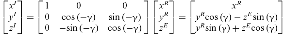 $$\begin{equation}
\left[ {\begin{array}{@{}*{1}{c}@{}} {{x^I}}\\ {{y^I}}\\ {{z^I}} \end{array}} \right] = \left[ {\begin{array}{l@{\quad}c@{\quad}c@{\quad}c} 1&0&0\\ 0&{{\rm{cos}}\left( { - \gamma } \right)}&{{\rm{sin}}\left( { - \gamma } \right)}\\ 0&{ - {\rm{sin}}\left( { - \gamma } \right)}&{{\rm{cos}}\left( { - \gamma } \right)} \end{array}}\!\!\!\!\! \right]\left[ {\begin{array}{@{}*{1}{c}@{}} {{x^R}}\\ {{y^R}}\\ {{z^E}} \end{array}} \right] = \left[ {\begin{array}{@{}*{1}{c}@{}} {{x^R}}\\ {{y^R}{\rm{cos}}\left( \gamma \right) - {z^E}{\rm{sin}}\left( \gamma \right)}\\ {{y^R}{\rm{sin}}\left( \gamma \right) + {z^E}{\rm{cos}}\left( \gamma \right)} \end{array}} \right]
\end{equation}$$
$$\begin{equation}
\left[ {\begin{array}{@{}*{1}{c}@{}} {{x^I}}\\ {{y^I}}\\ {{z^I}} \end{array}} \right] = \left[ {\begin{array}{l@{\quad}c@{\quad}c@{\quad}c} 1&0&0\\ 0&{{\rm{cos}}\left( { - \gamma } \right)}&{{\rm{sin}}\left( { - \gamma } \right)}\\ 0&{ - {\rm{sin}}\left( { - \gamma } \right)}&{{\rm{cos}}\left( { - \gamma } \right)} \end{array}}\!\!\!\!\! \right]\left[ {\begin{array}{@{}*{1}{c}@{}} {{x^R}}\\ {{y^R}}\\ {{z^E}} \end{array}} \right] = \left[ {\begin{array}{@{}*{1}{c}@{}} {{x^R}}\\ {{y^R}{\rm{cos}}\left( \gamma \right) - {z^E}{\rm{sin}}\left( \gamma \right)}\\ {{y^R}{\rm{sin}}\left( \gamma \right) + {z^E}{\rm{cos}}\left( \gamma \right)} \end{array}} \right]
\end{equation}$$
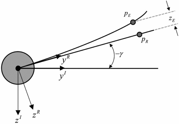
Figure 6. Rear view of the wing in flapping cycle.
5.3 Structural considerations
Given the employed modal approach in dynamic modelling of the structure, the developed equations are valid for all elastic wings with different geometrical shape and features as long as its modal properties, including natural frequencies and mode shapes are available. However, in order to better understand the implementation procedure, a rectangular wing case is investigated in this study.
The considered rectangular wing, Fig. 5, is modelled as cantilever structure. This is because the wing structure is practically being carried by the servomotor connector bar where the EFW is fixed to this connector bar at the junction. As discussed earlier, structural vibrations are obtained around the rigid instantaneous position of the wing and subsequently the inertial position of the wing elements will be computed via Equation (61)
Despite the fact that the extracted relations in Section 3.0 are independent of the structural elements type for FEM analysis, the EFW structure is considered as a Reinforced Rectangular Structure (RRS). The RRS is modelled as a flat plate with dimensions of 1(mm) × 300(mm) × 500(mm), reinforced at the Leading Edge (LE) by a tubular beam of radius 2 mm that adds to the flexural strength about the xR axis Further, the RRS Aluminium wing has stiffness properties E = 70 GPa, G = 26 GPa and a mass density of  $\rho = 2710\;{{{\rm{kg}}}
/ {{{\rm{m}}^3}}}$(Reference Beer, Russell, DeWolf and Mazurek48).
$\rho = 2710\;{{{\rm{kg}}}
/ {{{\rm{m}}^3}}}$(Reference Beer, Russell, DeWolf and Mazurek48).
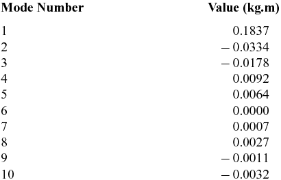
The modal properties are determined via FEM for 25 × 15 elements EFW, where the first 10 modes are taken into account, see Table 1 and Fig. 7. The pertinent values of the Generalised Inertial Moments are computed and tabulated in Table 2.
Table 1 Natural frequencies of first 10 structural modes
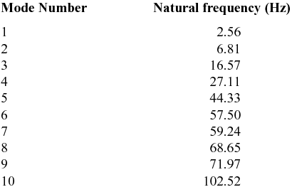
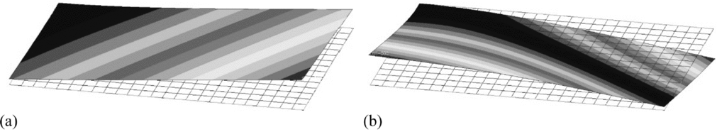
Figure 7. Wing displacement along z-axis regarding a) 1st and b) 2nd structural mode.
Table 2 Generalised inertial moment of first 10 structural modes
Generally in a beam-based modelling approach, the elastic axis is a line along which transverse loads only produce bending, while causing no sectional torsion at any spanwise station. Considering this concept, it can be deduced from Fig. 7 that both bending as well as torsional wing behaviours occur along an oblique line for the 1st and 2nd structural modes. This oblique line, in fact, shows the position of the elastic axis along the beam length or spanwise direction. This is an important issue often not attended to by researchers(Reference Su and Cesnik28,Reference De Rosis, Falcucci, Ubertini and Ubertini30,Reference Isogai and Harino39) utilizing the beam assumption in which the spanwise displacement of the elastic axis is neglected.
In order to verify the analytical structural solution of the EFW, the commercial Nastran-Patran(49) (NASP) FEM code is utilised whose transient response results for a time-dependent point force, (f(t) = 0.1 sin(2πt)) where 0 < t < 1 applied to point c (see Fig. 9) of the EFW, is shown in Fig. 8. This figure compares the analytically calculated elastic displacement of point c against the transient response result of NASP. As demonstrated in this figure, both results coincide and thus the proposed analytical solution is accurate and compatible with no-planner-displacement assumption.
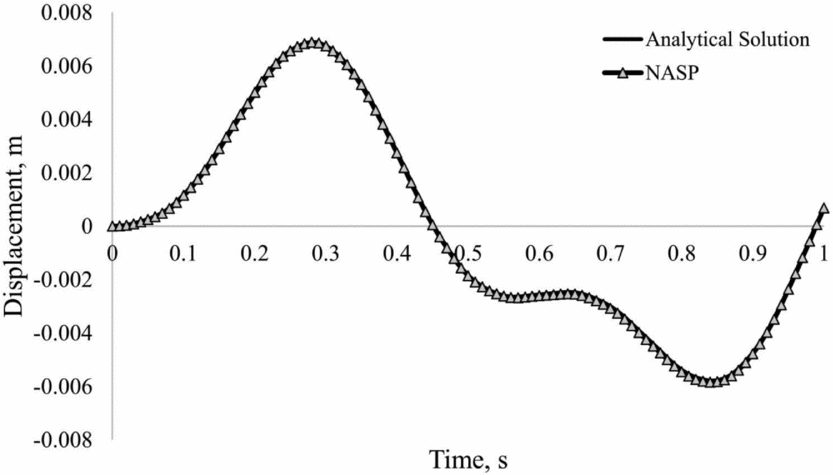
Figure 8. Elastic displacement of point c, from analytical solution versus the transient response in NASP.
5.4 Simulation and results
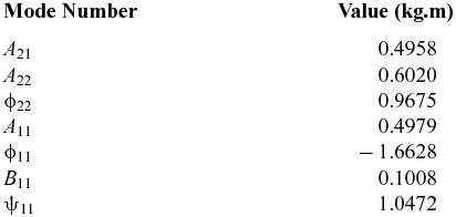
The EFW simulation parameters are listed in Table 3 that has resulted in the solution parameters (using Equations (21) and (Reference Nogar, Gogulapati, McNamara and Serrani32)) given in Table 4.
Table 3 EFW simulation parameters
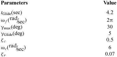
Table 4 Calculated solution parameters
According to the aforementioned flight scenarios, simulations of the EFW flapping and gliding motion are performed continuously and consecutively. It needs to be mentioned that the number of required modes is problem dependent and it is shown that three modes are sufficient. The effects of taking additional modes numbers for some typical wing nodes shown in Fig. 9 are analytically studied and reported in Figs 10 and 11. As can be seen from Fig. 9, point c is of highest displacement whose value sufficiently converges with only three modes with an accuracy level of better that 0.5 percent as demonstrated in Fig. 11.
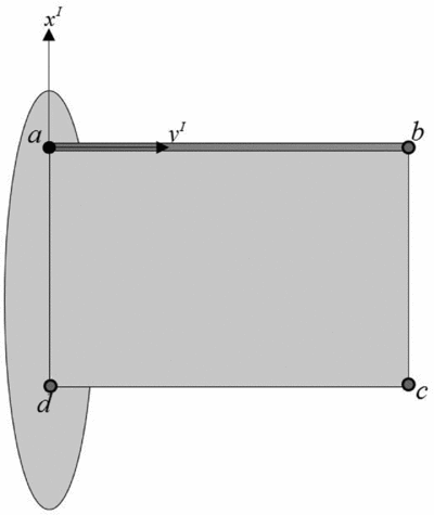
Figure 9. Sample selected nodes.
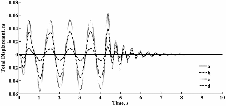
Figure 10. Cycle elastic displacements of the selected sample nodes using 10 modes.
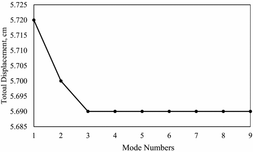
Figure 11. Displacement of point c versus number of modes.
Finally, the EFW motion is animated under the influence of the controller dynamics in Fig. 12 at different time steps. Another important observation that emanates out of Fig. 7, indicates that the selected EFW actually undergoes its bending and torsional motion along an oblique elastic axis. This observation demonstrates the complexity and dependency of the EFW dynamic behaviour on its geometric and structural features. Thus, in general, a one-dimensional beam-type model, usually chosen by many researchers(Reference Pourtakdoust and Karimain Aliabadi29,Reference Isogai and Harino39) , is improper for dynamic modelling of EFW behaviour unless the variation of elastic axis at each spanwise section is carefully considered. Still, this alone would not guarantee proper accuracy of EFW structural dynamic analysis, as chordwise geometric fluctuations have a great influence on aerodynamic properties of the aerofoil sections and consequently, the whole wing.
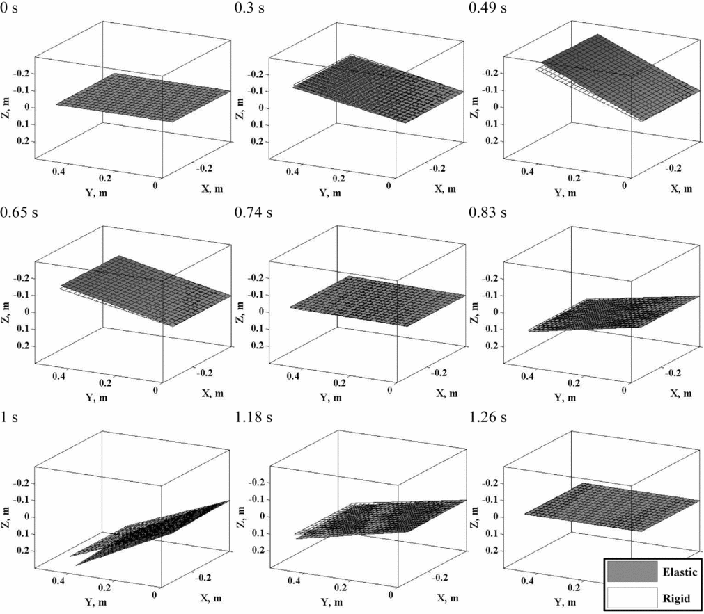
Figure 12. Wing status at first cycle in nine different step times.
6.0 CONCLUSION
An analytical SD solution of an EFW in Transient phase of Flapping and Gliding is presented using a modal approach. The solution is verified under a time-varying loading scenario. Due to the importance of the derivation of an analytical solution for EFW structural in order to conceptually analyse the effect of wing elasticity, the linear-motion range assumption is stipulated.
A common flight scenario of birds flying is simulated in which a wing starts a sinusoidal motion that is subsequently commended to stop at a fixed angular position while the servo dynamics is accounted for. As expected, the results show that the servo dynamics cause a delay as well as a change in the EFW motion amplitude. In the undamped systems, it is realized that resonance occurs if SFFR reach to one. On the other hand, the resonance won't happen in the damped system, but the maximum amplitude occurs when both frequency ratios i.e. SAFR and SFFR equal to one. Elastic sensitivity analyses reveals that one does not need to consider all structural modes, since the amplitudes pertinent to generalised coordinates of high-frequency modes tend towards zero. Another observation using FEM for the mode shapes indicated that both EFW bending and torsion behaviour occur about oblique lines. This is important when using beam assumption to model the elastic behaviour of the EFWs. The study also shows that one may substitute expensive numerical solution approaches by elegant mathematical based derivations for analysis. Although, because of importance and derivation of analytical results only inertial forces was considered, due to periodic nature of aerodynamic, they can be also taken into account using a similar mathematical methodology using a periodic series forcing such as the Fourier.
ACKNOWLEDGEMENTS
The authors would like to thank Dr. H. Haddadpour of Sharif University of Technology for his helpful suggestions in this study.


