2.2.1. Nonlinear model

In this study, the RANS equations are used to model the fluid flow. The one-equation Spalart–Allmaras turbulence model with the Edwards–Chandra modification is used to close the RANS equations system. This system reads in integral form

(2.5)\begin{equation} \boldsymbol{V} \frac{\partial \boldsymbol{W}}{\partial t} + \boldsymbol{R(\boldsymbol{W})} = 0, \end{equation}

where $\boldsymbol {W} = [\rho , \rho u , \rho v , \rho w ,\rho e , \rho \tilde {\nu }]^{t}$ is the conservative variables vector, $\boldsymbol {V}$ is a diagonal matrix whose non-zero coefficients are the mesh cells volume and $\boldsymbol {R}$ is the summation of the convective and viscous fluxes, and the source terms. In this article, $z$-invariant solutions (all the derivatives of the flow variables with respect to $z$ are null) with $w=0$ will be referred to as a 2-D solution, while $z$-invariant solutions with $w\neq 0$ will be referred to as 2.5-D solutions (Ghasemi, Mosahebi & Laurendeau Reference Ghasemi, Mosahebi and Laurendeau2014; Bourgault-Côté et al. Reference Bourgault-Côté, Ghasemi, Mosahebi and Laurendeau2017).

2.2.2. Linear model

Steady solutions $\boldsymbol {W}_0$ of (2.5), also known as baseflows, are computed to carry out global linear stability analyses (Sipp et al. Reference Sipp, Marquet, Meliga and Barbagallo2010; Theofilis Reference Theofilis2011; Taira et al. Reference Taira, Brunton, Dawson, Rowley, Colonius, McKeon, Schmidt, Gordeyev, Theofilis and Ukeiley2017). By definition, they satisfy $\boldsymbol {R}(\boldsymbol {W}_\textbf {0})=0$, and under a first-order approximation, infinitesimal perturbations $\boldsymbol {W}^{\prime }$ about a baseflow $\boldsymbol {W}_0$ are governed by the linearization of (2.5), which reads

(2.6)\begin{equation} \frac{\partial{\boldsymbol{W}^{\boldsymbol{\prime}}}}{\partial t} = \boldsymbol{A}\boldsymbol{W}^{\prime} ={-}\boldsymbol{V}^{{-}1} \left. \frac{\partial{\boldsymbol{R}}}{\partial{\boldsymbol{W}}}\right|_{\boldsymbol{W}_0}\boldsymbol{W}^{\prime} \end{equation}

where ${\partial {\boldsymbol {R}}}/{\partial {\boldsymbol {W}}}|_{\boldsymbol {W}_0}$ is the Jacobian of the discretized RANS equations evaluated about the baseflow, including the turbulence model. Solutions in the form of normal modes are sought;

(2.7)\begin{equation} \boldsymbol{W}^{\prime} = \textrm{e}^{\lambda t} \hat{\boldsymbol{W}}, \end{equation}

such that (2.6) reduces to the eigenproblem

(2.8)\begin{equation} \boldsymbol{A}\hat{\boldsymbol{W}} = \lambda\hat{\boldsymbol{W}}. \end{equation}

Thus, the stability problem consists in computing eigenpairs of the Jacobian operator. The eigenvectors $\hat {\boldsymbol {W}}$ describe the spatial structure of the global modes and the eigenvalues $\lambda = \sigma +\textrm {i}\omega$ describe their time behaviour $(i = \sqrt {-1})$. For each mode, the real part $\sigma$ is its growth rate and $\omega$ is its angular frequency.

2.3.1. Computational grids

Three-dimensional grids are obtained from the extrusion of baseline 2-D grids. Structured grids with an $O$-type topology are used. Table 1 reports the number of points on the aerofoil surface ($n_i$), in the direction normal to the aerofoil surface ($n_j$), on the pressures side ($n_{p.s.}$), on the suction side ($n_{s.s.}$), on the trailing edge ($n_{t.e.}$), the wall spacing (${\rm \Delta} y_w$), the distance from the aerofoil surface to the far-field boundary condition (${\rm \Delta} y_{f.f.}$) and the spacing across the shockwave (${\rm \Delta} x_{s.f.}$).

Table 1. Characteristics of the grids.

2.3.2. Solution of the nonlinear model

In this paper, the ONERA-Airbus-Safran elsA (Cambier, Heib & Plot Reference Cambier, Heib and Plot2013) software is used to solve the (U)RANS equations. For this study, a cell-centred structured finite volume method is used. A second-order cell-centred scheme with scalar numerical dissipation is used for the discretization of the convective fluxes. Convergence towards steady-state solutions is accelerated using local time steps and geometrical multigrid with a LU-SSOR pseudo-time integration scheme. In some case, selective frequency damping (SFD) (Åkervik et al. Reference Åkervik, Brandt, Henningson, Hoepffner, Marxen and Schlatter2006; Jordi, Cotter & Sherwin Reference Jordi, Cotter and Sherwin2014, Reference Jordi, Cotter and Sherwin2015; Richez, Leguille & Marquet Reference Richez, Leguille and Marquet2016) or a Newton solver (Wales et al. Reference Wales, Gaitonde, Jones, Avitabile and Champneys2012; Busquet et al. Reference Busquet, Marquet, Richez, Juniper and Sipp2017) is used to force the convergence to a steady state. Time-accurate solutions are obtained by using a second-order dual time stepping approach.

2.3.3. Solution of the linear model

This study involves 3-D geometries for which $\boldsymbol {A}$ has a high dimension and a large bandwidth. Therefore, solving the eigenproblem is often too costly. But in our cases, the baseflows are always homogeneous in the spanwise direction, such that the method proposed by Schmid, de Pando & Peake (Reference Schmid, de Pando and Peake2017) and used by Paladini et al. (Reference Paladini, Beneddine, Dandois, Sipp and Robinet2019a) and Plante et al. (Reference Plante, Dandois, Beneddine, Sipp and Laurendeau2019a) for $n$-periodic arrays of fluid systems may be used to significantly reduce the cost of the eigenvalues computation. This method exploits the block-circulant structure of matrix $\boldsymbol {A}$, which takes the form

(2.9)\begin{equation} \boldsymbol{A} =\begin{bmatrix} \boldsymbol{A}_0 & \boldsymbol{A}_1 & \boldsymbol{A}_2 & \ldots & \boldsymbol{A}_{n-1} \\ \boldsymbol{A}_{n-1} & \boldsymbol{A}_0 & \boldsymbol{A}_1 & \ldots & \boldsymbol{A}_{n-2} \\ \boldsymbol{A}_{n-2} & \boldsymbol{A}_{n-1} & \boldsymbol{A}_0 & \ldots & \boldsymbol{A}_{n-3} \\ \vdots & \vdots & \vdots & \ddots & \vdots \\ \boldsymbol{A}_1 & \boldsymbol{A}_2 & \boldsymbol{A}_3 & \ldots & \boldsymbol{A}_0\end{bmatrix} \end{equation}

when the degrees of freedom are properly indexed. As shown by Schmid et al. (Reference Schmid, de Pando and Peake2017), $\boldsymbol {A}$ can be transformed into a block diagonal matrix

(2.10)\begin{equation} \hat{\boldsymbol{A}} = \begin{bmatrix} \hat{\boldsymbol{A}}_0 & 0 & \cdots & 0 \\ 0 & \hat{\boldsymbol{A}}_1 & \ddots & \vdots \\ \vdots & \ddots & \ddots & 0 \\ 0 & \cdots & 0 & \hat{\boldsymbol{A}}_n-1 \end{bmatrix}\end{equation}

with

(2.11)\begin{equation} \hat{\boldsymbol{A}}_j = \sum_{k=0}^{n-1} \rho_j^{k} \boldsymbol{A}_k \end{equation}

and

(2.12)\begin{equation} \rho_j = \textrm{e}^{ij({2{\rm \pi}}/{n})}. \end{equation}

Eigenvalues of $\hat {\boldsymbol {A}}$ are also eigenvalues of $\boldsymbol {A}$ and each block matrix $\hat {\boldsymbol {A}}_{\boldsymbol {j}}$ can be treated separately, resulting in $n$ separated eigenproblems of the size of a 2-D problem,

(2.13)\begin{equation} \hat{\boldsymbol{A}}_{\boldsymbol{j}} \boldsymbol{v}_j = \lambda_j \boldsymbol{v}_j. \end{equation}

The eigenvectors of $\boldsymbol {A}$ are then retrieved as

(2.14)\begin{equation} \hat{\boldsymbol{W}} = \left[\boldsymbol{v}_j , \rho_j\boldsymbol{v}_j , \rho_j^{2}\boldsymbol{v}_j, \ldots, \rho_j^{n-1}\boldsymbol{v}_j\right]^{t}. \end{equation}

This method implies solving the eigenproblem for all the $\hat {\boldsymbol {A}}_j$ matrices to get the stability result for all the $n$ possible wavenumbers. However, the only difference between each $\hat {\boldsymbol {A}}_j$ matrix is the coefficients $\rho _j$ such that changing the value of $j$ or $n$ has the effect of changing the wavenumber. Hence, solving for the matrix $\hat {\boldsymbol {A}}_2$ is equivalent to solving $\hat {\boldsymbol {A}}_1$ with $n$ divided by two. Therefore, in this study, the problem is only solved for the matrix $\hat {\boldsymbol {A}}_1$ with various values of $n$. This allows us to get the results over a continuous range of wavenumbers.

This analysis yields results similar to the biGlobal stability analysis carried out by Crouch et al. (Reference Crouch, Garbaruk and Strelets2019) and He et al. (Reference He, Gioria, Pérez and Theofilis2017). However, this approach presents several advantages. In particular, it does not require tedious mathematical developments to include the periodicity assumption in the Jacobian matrix. This makes this approach suitable for the use of a black box computational fluid dynamics solver, in this case elsA.

The linear operator $\boldsymbol {A}$ is obtained with the fully discrete approach proposed by Mettot, Renac & Sipp (Reference Mettot, Renac and Sipp2014). This Jacobian is extracted with a second-order finite difference scheme as

(2.15)\begin{equation} \boldsymbol{A}\boldsymbol{u} \approx \frac{1}{2\epsilon}\left(\boldsymbol{R}(\boldsymbol{W}_\textbf{{0}}+ \epsilon\boldsymbol{u})-\boldsymbol{R}(\boldsymbol{W}_\textbf{{0}}-\epsilon\boldsymbol{u})\right), \end{equation}

where $\epsilon$ is a small parameter and $\boldsymbol {u}$ are vectors chosen to efficiently compute every non-zero coefficient of the Jacobian matrix (see Beneddine (Reference Beneddine2017) for details). For the second-order finite volume scheme used in this study, the numerical stencils have a width of five grid cells. Hence, $\boldsymbol {A}_3 = \boldsymbol {A}_4 = \cdots = \boldsymbol {A}_{n-3} = 0$, and all the non-zero block matrices $\boldsymbol {A}_j$ (2.9) can be retrieved from a 3-D grid with only five grid cells in the spanwise direction (see Paladini et al. Reference Paladini, Beneddine, Dandois, Sipp and Robinet2019a; Plante et al. Reference Plante, Dandois, Beneddine, Sipp and Laurendeau2019a). Hence, the baseflows are computed as 2-D solutions and the grid is extruded to get the 3-D mesh for the extraction of the 3-D Jacobian $\boldsymbol {A}$. The spanwise spacing ${\rm \Delta} z$ must be imposed. Refinement study of this parameter will be presented, but no extra computational cost is associated with a change in ${\rm \Delta} z$, which can therefore be chosen arbitrarily small. This Jacobian matrix is then reduced as $\boldsymbol {\hat {A}_1}$ by assuming a given wavenumber in (2.11). The eigenproblems are then solved with the Arnoldi iteration method (Sorensen Reference Sorensen1992) coupled with a shift-and-invert strategy (Christodoulou & Scriven Reference Christodoulou and Scriven1988) to extract inner eigenvalues.

3.1.1. Unswept $\delta =0^{\circ }$ case

Let us first focus on the flow over an unswept wing in the post-stall regime. Figure 2 shows the lift polar in the unswept case ($\delta =0^{\circ }$) for two kinds of simulations: 2-D solutions and 3-D solutions with an aspect ratio $AR=6$ and 113 spanwise grid points. The maximum lift coefficient of 1.57 is obtained for an angle of attack around $\alpha =14^{\circ }$ in both cases. For angles of attack higher than $16^{\circ }$ the flow solver failed to converge. This is caused by the occurrence of an instability linked to a vortex shedding. This is further discussed in § 4.1.4. In order to obtain steady-state 2-D solutions in this regime, the SFD method presented by Richez et al. (Reference Richez, Leguille and Marquet2016) and the Newton algorithm have been used. The SFD is used with a local time stepping algorithm and the cut-off frequency and damping coefficient were based on a parametric study to obtain solutions converged within machine accuracy. A value of the filter width $\varDelta = 1/74$ and the proportional controller coefficient $\chi =50$ allowed the solution to converge, and the Courant–Friedrichs–Lewy number is set to 50 to compute the local time step in the LU-SSOR implicit scheme. To ensure consistency, it has been checked that both methods provide the same solution for several cases. Successive solutions are obtained by initialising each computation from the previous angle of attack. The lower branch of the lift polar is obtained by increasing the angle of attack up to values for which a converged solution could no longer be obtained. Then, by decreasing the angle of attack starting from these unconverged flow solutions, the solution method is able to converge on the lower branch of the lift curve. Every solution has been converged within machine accuracy. Two distinct solutions are found for some angles of attack. Such hysteresis phenomena of the discretized RANS equations were obtained by Wales et al. (Reference Wales, Gaitonde, Jones, Avitabile and Champneys2012) and Busquet et al. (Reference Busquet, Marquet, Richez, Juniper and Sipp2017) for the NACA0012 and the OA209 aerofoils, respectively. Grid convergence has been ensured by carrying out a 2-D simulation at an angle of attack of $15^{\circ }$ with a grid refined by a factor 2 in both directions (1024 by 256 grid cells), resulting in non-significant differences in the pressure distribution.

Figure 2. Lift curve for the 2-D and 3-D steady solutions (NACA4412, $Re=350\,000$, $M=0.2$, $\delta =0^{\circ }$).

For angles of attack over $14^{\circ }$ the 3-D lift coefficient is lower than the 2-D one. These solutions are obtained using a global time step and the SFD technique. The lower lift coefficient is associated with the presence of stall cells, as seen in figure 3 for an angle of attack of $15^{\circ }$. Four steady stall cells are observed and the skin friction lines exhibit the ‘owl face’ shape reported in the literature. The left-hand part of this figure shows the result with a spanwise mesh refinement of a factor 2. No significant change in the result is noticeable, ensuring the grid convergence of the results. In this simulation, the wavenumber of the stall cell is $4.2$. However, the periodic boundary conditions constrain the possible wavenumbers since the number of cells must be an integer. Hence, the only possible wavenumbers that may appear in the simulation are necessarily multiples of $\beta _0=2{\rm \pi} /6$. There might therefore exist a discrepancy with respect to a truly infinite configuration, with $AR=\infty$. A more accurate estimation of the most amplified wavenumber may be obtained by considering a larger aspect ratio. For this reason, a simulation with $AR=12$ has also been run and eight stall cells were obtained. Therefore, the most amplified wavenumber is narrowed down to a value between $14{\rm \pi} /12 \approx 3.7$ and $18{\rm \pi} /12 \approx 4.7$. This range will be compared with the result of linear stability analyses in § 4.1.

Figure 3. Surface pressure coefficient and skin friction lines of 3-D steady solution with 224 (left-hand side) and 112 (right-hand side) spanwise grid cells (NACA4412, $M=0.2$, $Re=350\,000$, $\alpha =15^{\circ }$, $\delta =0^{\circ }$, $L_z=6$).

Since the 2-D solutions are particular cases where every derivative in the spanwise direction are null, they are also solutions of the 3-D discretized RANS equations. Hence these results demonstrate the existence of multiple solutions, the 2-D and the 3-D ones, for a given flow conditions. Such results are in agreement with those from Kamenetskiy et al. (Reference Kamenetskiy, Bussoletti, Hilmes, Venkatakrishnan, Wigton and Johnson2014).

3.1.2. Swept cases $\delta >0^{\circ }$, $\alpha =15^{\circ }$

A fixed value $\alpha =15^{\circ }$ is now considered and a sweep angle is added. In these conditions, the flow is unsteady and time-accurate simulations with a non-dimensional time step of 0.008 are carried out. Figure 4 shows the instantaneous pressure coefficient and the skin friction lines over wings swept at $10^{\circ }$, $20^{\circ }$ and $30^{\circ }$. Four stall cells are observed and the wavenumber is the same as for the unswept wing ($\beta = 4.2$). The topology of the stall cells also changes with the sweep angle, and the skin friction lines are now aligned in the cross-flow direction. This is associated with a spanwise convection of the stall cells. This induces a frequency proportional to the wavelength of the cells and their convection speed ($St = {V_C}/{\lambda _z}$). Table 2 summarizes all the wavelength and convection speed obtained for sweep angles of $0^{\circ }$, $10^{\circ }$, $20^{\circ }$ and $30^{\circ }$. Figure 5 shows the definition of these quantities. For the simulations at a constant aspect ratio, the wavenumber is always 4.2. These results suggest that the sweep angle has no effect on the wavelength of the stall cells. However, as mentioned previously, this result is constrained by the wing aspect ratio. Finally, the convection speed observed in the URANS results is proportional to the sweep angle. These phenomena are also analysed using stability analyses in § 4.1.3.

Figure 4. Instantaneous surface pressure coefficient and skin friction lines over a swept wing (NACA4412, $M=0.2$, $Re=350\,000$, $\alpha =15^{\circ }$, $L_z=6$): (a) sweep $10^{\circ }$; (b) sweep $20^{\circ }$; (c) sweep $30^{\circ }$.

Table 2. Stall cells convection frequency for several wing spans and sweep angles (NACA4412, $M=0.2$, $Re=350\,000$, $\alpha =15^{\circ }$).

Figure 5. Stall and buffet cells convection model.

3.2.1. Spanwise invariant solutions (2.5-D)

Figure 6 shows the time-averaged wall pressure coefficient of 2-D and 2.5-D simulations. The pressure coefficient on the pressure side and the trailing edge agree with the experiments of Brion et al. (Reference Brion, Dandois, Abart and Paillart2017) and the pressure of the supersonic plateau is also the same. This indicates that the Mach number and angle of attack are the same between the experiments and the simulations. However, the shock wave of the simulations is located further downstream compared with the experimental field. It is seen that the pressure distribution is the same for every sweep angle, except in the shock wave region. This shows that the flow fields in the $(x,y)$ plane remain close due to the fact that the upstream normal inflow conditions are kept constant when changing the sweep angle. The time evolution of the lift coefficient yields a Strouhal number of 0.075. The shock wave motion amplitude can be evaluated from the slope of the time-averaged pressure coefficient in the vicinity of the shock wave position. The largest buffet amplitude is observed for the unswept case and the buffet amplitude decreases as the sweep angle is increased. This relation between the sweep angle and the buffet amplitude is investigated with global stability analyses in § 4.2.3.

Figure 6. Time-averaged wall pressure coefficient for spanwise invariant solution with several sweep angles (OALT25, $M=0.7352$, $Re=3\times 10^{6}$, $\alpha = 4^{\circ }$).

3.2.2. Superposition between 2-D buffet mode and 3-D buffet cells

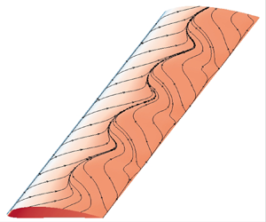
Figure 7 shows the instantaneous pressure coefficient and skin friction lines on swept wings of aspect ratio $AR = 6$ meshed with 168 spanwise grid cells. For the unswept wing and the wing swept at $30^{\circ }$, a variation of the shock wave position is observed, forming the so-called buffet cells. For the unswept wing $(\delta =0^{\circ })$, spanwise structures are observed. However, the amplitude of the buffet cells is irregular and the number of buffet cells varies in time. As such, the wavenumber varies in time and the buffet cells appear and disappear at random spanwise location since there is no convection. This results in a flow that can seem chaotic but a dominant Strouhal number of 0.06 is observed. This is related to the frequency of a chordwise variation of the shock wave position and a variation of the buffet cells’ amplitude. The same frequency is observed for swept wings ($\delta >0^{\circ }$). However, in these cases the number of buffet cells is constant and they are convected in the spanwise direction. Two cells are observed for a sweep angle of $\delta =30^{\circ }$. This result is compared with the stability analysis results in § 4.2. Figure 7 also shows the instantaneous solution with 112 and 168 spanwise grid cells. The comparison of the two fields shows that the grid spacing is sufficient for this case since no significant differences are noticeable in the skin friction lines and the pressure coefficient.

Figure 7. Instantaneous surface pressure coefficient and skin friction lines for URANS simulations of infinite swept wings with two sweep angles (OALT25, $M=0.7352$, $Re=3\times 10^{6}$, $\alpha =4^{\circ }$, $L_z=6$): (a) $\delta =0^{\circ }$; (b) $\delta =30^{\circ }$ (right-hand side, 112 spanwise grid cells; left-hand side, 168 spanwise grid cells).

Figure 8 shows the power spectral density of the sectional lift coefficient with 112, 168 and 224 spanwise grid cells. The sectional lift coefficient is extracted on a given chordwise wing section, the choice of this section has no effect since the buffet cells are convected in the spanwise direction. The sectional lift coefficient is sampled at every time step (0.0105 non-dimensional time unit) over a time frame of 630 non-dimensional time units. A periodogram with boxcar window and a single block is used to estimate the power spectral density, which yields a Strouhal number resolution of 0.00158. This method is used since the signals for the grid refinement study are too short to use a sufficient number of averaging blocks. This yields noisier spectra and estimation errors on the amplitude. Nevertheless, one can observe that the peak frequencies are the same. A dashed line is added to indicate the Strouhal number around 0.06 (the frequency observed for every sweep angle) and a dashed-dotted line indicates the Strouhal number of 0.135. The latter is associated with the convection of buffet cells, as it will be shown in this section. Another peak at a frequency of 0.135 could correspond to the nonlinear interaction between the two dominant modes ($St = 0.135+0.055 = 0.19$).

Figure 8. Sectional lift coefficient power spectral density (OALT25, $M=0.7352$, $Re=3\times 10^{6}$, $\alpha =4^{\circ }$, $\delta =30^{\circ }$).

Figure 9 shows the power spectral density of the sectional and global lift coefficient with sweep angles of $10^{\circ }$, $20^{\circ }$ and $30^{\circ }$. These spectra are evaluated using the Welch method with a Hann window and a 50 % overlap between the blocks. The signal length is of $1\,260$ non-dimensional time units and nine blocks are used. The Welch method is used since the time series is longer than in the mesh refinement study. The sampling is done at every time step (0.0105 non-dimensional time units) for the sectional lift and every 10 time steps for the global lift. This yields a Strouhal number resolution of 0.0039. One can notice the frequency between $St = 0.055$ and $0.06$ indicated by a dashed line for every sweep angle in the global and sectional lift signals. Some harmonics of this frequency are also observed. This frequency is associated with a chordwise oscillation of the shock wave position which modulates the buffet cells amplitude (2-D oscillation). However, a second dominant frequency is observed in the sectional lift coefficient. The latter increases with the sweep angle and is due to the buffet cells convection in the spanwise direction. This second frequency is not observed in the spectrum of the global lift coefficient since the number of buffet cells is constant. For this reason, the variations of the lift coefficient associated with the convection are cancelled out when the lift coefficient is averaged along the span. Like in figure 8, the dashed line indicates the 2-D shock oscillation phenomenon while the dashed-dot lines indicates the buffet cells’ convection phenomenon. These two frequencies are further discussed in the next paragraph. Some harmonics of the buffet cells convection frequency are also observed. For instance the convection Strouhal number of 0.045 for a sweep angle of $10^{\circ }$ has a harmonic at 0.09, which is also the convection frequency for a sweep angle of $20^{\circ }$.

Figure 9. Effect of the sweep angle on the global and sectional lift coefficient power spectral density (OALT25, $M=0.7352$, $Re=3\times 10^{6}$, $\alpha =4^{\circ }$).

To visualize the unsteady behaviour of the flow, the pressure has been extracted along a line parallel to the leading edge. Figure 10 is a ($z, t$) diagram showing this extraction of the pressure coefficient near ${x^{\prime }}/{c} = 0.43$ for the sweep angle of $30^{\circ }$. Most of the time, the pressure is equal to the one on the supersonic plateau. However, two buffet cells periodically cross the extraction line because the amplitude of the cells changes in time. This occurs with a period $T = 18.0$. This results in a Strouhal number equal to 0.055 (around the Strouhal number of 0.06 shown in figure 9). A Strouhal number of this order is observed for every sweep angle, as previously shown, thus suggesting that the variation of the buffet cells amplitude relates to a 2-D buffet mode. In addition, this figure allows us to follow the spanwise location of the buffet cells in time. Hence, the convection speed of the buffet cells can be extracted as the slope of an isocontour of pressure on this pressure map (here $V_C = 0.4$) and the associated frequency can be computed with the wavelength of the buffet cells ($St = {V_C}/{\lambda _z}$). These quantities are schematized in figure 5 and reported for multiple sweep angles in table 3. Figure 11 shows the relation between the sweep angle and the convection speed. The cross-flow velocity varies in $\tan \delta$, meaning that the convection speed is proportional to the far field velocity projected along the leading edge. This proportionality is true for low-speed flow conditions as well. A fit coefficient of 0.7 is found for the buffet cells and 0.8 for the stall cells. More details are provided in Plante et al. (Reference Plante, Dandois and Laurendeau2019b). This relation between the sweep angle and the convection speed of the buffet cells is further analysed using stability analyses in § 4 for the stall and buffet conditions.

Figure 10. Extraction of the pressure on a line parallel to the leading edge near ${x^{\prime }}/{c} = 0.43$ (OALT25, $M=0.7352$, $Re=3\times 10^{6}$, $\alpha =4^{\circ }$, $\delta =30^{\circ }$).

Table 3. Buffet cells convection frequency for several sweep angles (OALT25, $M=0.7352$, $Re=3\times 10^{6}$, $\alpha =4^{\circ }$).

Figure 11. Convection speed of stall (NACA4412, $M=0.2$, $Re=350\,000$, $\alpha =15^{\circ }$) and buffet (OALT25, $M=0.7352$, $Re=3\times 10^{6}$, $\alpha =4^{\circ }$) cells.

4.1.1. Case $\delta =0^{\circ }$ and $\alpha =15^{\circ }$

The following focuses on the case $\delta =0^{\circ }$ and $\alpha =15^{\circ }$. Figure 12 presents the eigenvalues spectra obtained for two values of $\beta$. For both values, there is an unstable eigenvalue (positive real part) located along the real axis. This is a non-oscillatory unstable mode. A mode similar to this one has been observed by Zhang & Samtaney (Reference Zhang and Samtaney2016) for low-Reynolds laminar flow. But in the present case this mode is observed at an intermediate Reynolds number with the use of a steady RANS baseflow. This figure also shows the radius covered by the shift-and-invert Arnoldi strategy. Different shifts with various imaginary parts are used in the shift-and-invert strategy to ensure that modes with non-zero imaginary part are not missed. Figure 13 shows the growth rate of the steady unstable mode for a range of wavenumbers $\beta$. Multiple values of $\varDelta _z$ used in the extrusion of the grid are plotted to ensure that the grid is sufficiently refined. These results can be considered converged for every $\beta$ with $\varDelta _z=0.002$. One can observe that the grid convergence is poorer in the high $\beta$ range associated with small structures. This indicates that a finer grid is required to compute small flow structures, as expected. The grid spacing used in the URANS simulations ($\varDelta _z = 0.054$) is well converged up to $\beta = 6$, covering the case with the maximum growth rate and the wavenumbers obtained in the URANS simulations. This is consistent with the grid convergence shown in figure 3.

Figure 12. Eigenspectrum (NACA4412, $M = 0.2$, $Re = 350\,000$, $\alpha$ = $15.0^{\circ }$, $\delta = 0.0^{\circ }$).

Figure 13. Effect of spanwise grid density and the wavenumber on the growth rate of the unstable mode (NACA4412, $M = 0.2$, $Re = 350\,000$, $\alpha = 15.0^{\circ }$, $\delta = 0.0^{\circ }$).

The maximum growth rate is obtained for a spanwise structure with $\beta \approx 4.4$. This corresponds to a wavelength $\lambda _z \approx 1.43$, which is consistent with the value observed in the URANS simulations $(\beta = 4.2)$. Indeed, in the simulations, the periodic boundary conditions constrained the possible wavenumbers to multiples of $\beta _0=2{\rm \pi} /AR$. Therefore, the wavelength of the URANS simulation is as close as possible to that predicted by the stability analysis, showing that this unstable mode is responsible for the formation of stall cells. Figure 14 shows the baseflow and the real part of the eigenvector $\widehat {\rho e}$ reconstructed in three dimensions with (2.14), and extracted on the aerofoil surface and the plane $z=0$. The instability is located in the shear layer and upstream of the separation line. The shape of this mode is consistent with the structure of the stall cells.

Figure 14. Flow visualization of the (a) baseflow and (b) 3-D unstable mode (NACA4412, $M = 0.2$, $Re = 350\,000$, $\alpha = 15.0^{\circ }$, $\delta = 0.0^{\circ }$): (a) ${\rho e}/{\rho e_{\infty }}$ baseflow; (b) real part of the ${\widehat {\rho e}}/{\rho e_{\infty }}$ eigenmode $(\beta = 4.4) - St = 0.0$.

4.1.2. Case $\delta =0^{\circ }$ and varying $\alpha$

These stability analyses are carried out for several angles of attack for which a solution converged to machine accuracy can be obtained (figure 2). The 3-D unstable mode can be identified on the upper and lower branch of the lift polar hysteresis. Figure 15 shows the growth rate of this mode for the most amplified wavenumber of the two branches. The mode is unstable from an angle of attack of $14.15^{\circ }$ (the maximum lift) up to $20.5^{\circ }$ (the last converged baseflow). On the lower branch, the growth rates are higher than for the upper one, but the mode is only unstable for angles of attack lower than $16.9^{\circ }$. Above this angle, the mode becomes stable again, even though the flow is massively separated. Figure 16 shows the shape of the modes on the upper and lower branches. One can observe that the unstable mode is located around the region where the flow separates. For $\alpha = 18^{\circ }$ the flow separates far from the leading edge. However, for the other angles of attack the separation is close to the leading edge. Hence, it is possible that the mode is no longer unstable past $\alpha = 16.9^{\circ }$ on the lower branch because the flow separation becomes fixed on the leading edge. This tends to validate the idea that stall cells are only observed with a trailing edge type of stall.

Figure 15. Effect of the angle of attack on the growth rate of the unstable mode (NACA4412, $M = 0.2$, $Re = 350\,000$, $\delta = 0.0^{\circ }$). (a) Upper branch of the lift hysteresis. (b) Lower branch of the lift hysteresis.

Figure 16. Flow visualization of the 3-D unstable mode for several angles of attack on the two branches of the lift hysteresis (NACA4412, $M = 0.2$, $Re = 350\,000$, $\delta = 0.0^{\circ }$). (a) Real part of the ${\widehat {\rho e}}/{\rho e_{\infty }}$ eigenmode ($\alpha =18^{\circ }$, upper branch, $\beta = 5$) – $St = 0.0$. (b) Real part of the ${\widehat {\rho e}}/{\rho e_{\infty }}$ eigenmode ($\alpha =20.5^{\circ }$, upper branch, $\beta = 7.5$) – $St = 0.0$. (c) Real part of the ${\widehat {\rho e}}/{\rho e_{\infty }}$ eigenmode ($\alpha =16.78^{\circ }$, lower branch, $\beta = 8$) – $St = 0.0$. (d) Real part of the ${\widehat {\rho e}}/{\rho e_{\infty }}$ eigenmode ($\alpha =16.9^{\circ }$, lower branch, $\beta = 5.5$) – $St = 0.0$.

Works based on the lifting line theory by Spalart (Reference Spalart2014) and Gross et al. (Reference Gross, Fasel and Gaster2015) suggested that a negative slope of the $C_L-\alpha$ curve is a necessary condition for the occurrence of stall cells. Figure 15 shows the growth rate obtained in these flow conditions for different values of $\alpha$, and for the upper branch of the lift hysteresis, the most unstable eigenvalue crosses the imaginary axis at an angle of attack slightly below $14.15^{\circ }$. This coincides with the maximum lift angle of attack in figure 2, which is therefore consistent with the negative $C_L-\alpha$ slope criterion. However, the stability analysis of the lower branch of the lift hysteresis shows that the stall cell modes are stable for $\alpha >16.9^{\circ }$, while the slope of the $C_L-\alpha$ curve is negative between $17.0^{\circ }$ and $17.4^{\circ }$ (see figure 2), which contradicts this criterion. Another conclusion of the analysis of Gross et al. (Reference Gross, Fasel and Gaster2015) is that the wavelength of the cells should be $\lambda _z = -0.5({\partial C_L}/{\partial \alpha })$ with a discrete model or $\lambda _z = -({{\rm \pi} }/{4})({\partial C_L}/{\partial \alpha })$ with a continuous model. Since the linear instability occurs around the 2-D solution, ${\partial C_L}/{\partial \alpha }$ is taken as the slope of the 2-D lift polar around an angle of attack of $15.0^{\circ }$ ($-2.52\ \textrm {rad}^{-1}$). With this slope, the wavelength should be 1.26 or 1.98 ($\beta =3.2$ and $5.0$, respectively). The values computed with the URANS ($\beta = 4.2$) simulations and the stability ($\beta = 4.4$) analyses fall between the values predicted with this model. However, the $C_L-\alpha$ slope varies in the range of angles of attack studied with the global stability analysis and the values of $\beta$ for which the flow is the most unstable does not vary significantly. This is in contradiction with the model proposed by Gross et al. (Reference Gross, Fasel and Gaster2015).

4.1.3. Effect of sweep at $\alpha =15^{\circ }$

The approach followed to carry out stability analyses also enables to study baseflow with $\delta \neq 0$. Figures 17(a) and 17(b) show the growth rate and frequency of the unstable mode with sweep angles of $0^{\circ }$, $10^{\circ }$, $20^{\circ }$, $30^{\circ }$ and $40^{\circ }$. With these curves, it is possible to track the displacement of the most unstable eigenvalue with respect to the sweep angle. The frequency of the mode increases with the sweep and its growth rate decreases. For a sweep angle between $40^{\circ }$ and $50^{\circ }$, the mode becomes stable. The value of $\beta$ for which the growth rate is maximum also slightly decreases as the sweep angle increases. The stability results are consistent with the URANS simulations from § 3. For example, the wavenumber observed in figure 3 in the unswept case is 4.2 with four stall cells. By accounting for the numerical constraint on the wavenumber (the domain size imposes the possible values of $\beta$), the actual wavenumber on an infinite domain is expected to be between 3.7 and 4.7. The modes with the maximum growth rate have $\beta$ between 4.0 and 4.4, hence within the expected range.

Figure 17. Effect of the sweep angle on the growth rate and frequency of the 3-D unstable mode (NACA4412, $M = 0.2$, $Re = 350\,000$, $\alpha = 15.0^{\circ }$; black, stability analysis; red, URANS simulations): (a) growth rate; (b) frequency.

Figure 17(b) also shows the frequency obtained with URANS simulations (red points) and the frequency extrapolated from the trend of the convection speed (see figure 11) and the wavenumber (red lines). The frequencies observed in the URANS computations are well aligned with the frequency obtained with the global linear stability analysis. Hence, the linear stability analyses predict the behaviour of the stall cells.

4.1.4. 2-D wake instability mode

These analyses are now carried for $\beta = 0$, which corresponds to 2-D analyses. Such analyses are performed for several angles of attack. Figure 18 shows the part of the spectra where unstable modes are found. The mode becomes unstable for an angle of attack between $16^{\circ }$ and $17^{\circ }$ for the upper branch (UB) of the lift hysteresis, and is unstable for the entire lower branch (LB). This is consistent with the need to use the SFD technique or a Newton solver to converge the baseflow for angles of attack above $16^{\circ }$, where it was observed that the local time stepping technique failed to converge. Figure 19 shows the eigenmodes for the upper and lower branch of the lift hysteresis at an angle of attack of $18^{\circ }$. The shape of these modes corresponds to a meandering of the wake which would lead to shedding of vortices in the nonlinear regime. The wavelength of this mode is larger for the lower branch, where the size of the separation is larger. As the angle of attack increases, the size of the separation region becomes larger and the Strouhal number based on the chord length ($St_c$) decreases. However, the Strouhal number based on the frontal height of the separation zone ($St_l = St_c l = St_c(x_{r}-x_{s})\sin \alpha$) stays constant around 0.2. This Strouhal number definition based on the separation height is inspired from the one of Yon & Katz (Reference Yon and Katz1998) and Zaman, McKinzie & Rumsey (Reference Zaman, McKinzie and Rumsey1989), but adapted to the case where the separation point $x_{s}$ is not located at the leading edge but somewhere between the leading and the trailing edge; here the flow reattaches at the trailing edge ($x_{r} = 1.0$). This shows that the Strouhal number based on the separation height is the correct one and its value is close to the expected one for vortex shedding (Chabert, Dandois & Garnier Reference Chabert, Dandois and Garnier2016). Hence, for $\alpha \gtrapprox 16.5^{\circ }$, the 3-D non-oscillating mode coexists with a 2-D wake instability mode, such that an unsteady behaviour should be observed in the URANS simulations. On the other hand, the case $\alpha =15^{\circ }$ was analysed in § 3.1, and consistently with the stability results (only the 3-D steady mode is unstable for this value of $\alpha$), the unsteady computation converges toward a steady state. Hence, once again, the results of § 3 are consistent with the stability analyses.

Figure 18. Effect of the angle of attack on the spectra of the 2-D unstable mode (NACA4412, $M = 0.2$, $Re = 350\,000$, $\delta = 0.0^{\circ }$, $\beta = 0$).

Figure 19. Flow visualization of the (a,b) baseflow and (c,d) 2-D unstable mode on the two branches of the lift hysteresis (NACA4412, $M = 0.2$, $Re = 350\,000$, $\alpha = 18.0^{\circ }$, $\delta = 0.0^{\circ }$, $\beta = 0.0$). (a) The $u$ baseflow; upper branch of the lift hysteresis. (b) The $u$ baseflow; lower branch of the lift hysteresis. (c) Real part of the $\widehat {\rho u}$ eigenmode; upper branch of the lift hysteresis – $St = 0.92$. (d) Real part of the $\widehat {\rho u}$ eigenmode; lower branch of the lift hysteresis – $St = 0.49$.

4.1.5. Effect of sweep angle on the 2-D wake instability mode

The same stability analyses are now carried out for sweep angles of $0^{\circ }$, $10^{\circ }$, $20^{\circ }$ and $30^{\circ }$ and an angle of attack of $18^{\circ }$. Figure 20 shows the value of the growth rate and the Strouhal number of the wake instability mode for values of $\beta$ around zero. This unstable mode exists for large wavenumbers $\beta$. In these figures, modes with a negative value of $\beta$ are shown. These modes can also be seen as modes with positive $\beta$ and a negative frequency. One can observe that, as expected, the spectrum is symmetric with respect to the imaginary axis when the sweep angle is null. In this case, the baseflow indeed exhibits a zero spanwise velocity and perturbations may equivalently propagate (in terms of phase, the phase-speed being $v_\phi =\omega /\beta$) towards the inboard (negative $z$, $v_\phi <0$) and outboard (positive $z$, $v_{\phi }>0$) directions. If a positive sweep is considered, then a positive baseflow velocity in the $z$ direction is added and the phase of the perturbation is generally preferentially advected in this direction (in the case of a constant $W(x,y)=W$ baseflow velocity, one can show that the frequency $\omega$ (respectively, phase-speed $v_\phi$) of a mode just shifts by an amount of $\beta W$ (respectively, $W$), due to the Doppler shift). Therefore, a positive sweep generally tends to increase the frequency of 3-D perturbations and their phase speed. For exactly 2-D oscillating perturbations (as obtained for the wake instability mode), the phase velocity is infinite (positive or negative), even if sweep is added. It is also seen that, if the perturbations become slightly 3-D ($\beta \neq 0$), then the outboard propagating 3-D perturbations are slightly more unstable than the inboard propagating ones. Note that the discussion would have been different if the group velocity ($v_g=\textrm {d}\omega /\textrm {d}\beta$) was considered, since the group velocity determines the speed of the envelope and fronts of a wave-packet and therefore better accounts for actual propagation of the perturbation: for this a convective/absolute stability analysis should be conducted following Huerre & Monkewitz (Reference Huerre and Monkewitz1990). But this is outside the scope of this paper.

Figure 20. Effect of the wavenumber on the 2-D wake instability mode (NACA4412, $M = 0.2$, $Re = 350\,000$, $\alpha = 18.0^{\circ }$): (a) growth rate; (b) frequency.

4.2.1. Effect of the angle of attack on the unswept case

Figure 21 shows the spectra obtained for $\beta = 2{\rm \pi}$ and $\beta = 0$ for an angle of attack of $4^{\circ }$ and a sweep angle of $0^{\circ }$. The cases where $\beta$ tends to 0 are equivalent to the 2-D cases. As one can see, an unstable global mode is found at a Strouhal number of 0.075 when $\beta = 0$ (unsteady 2-D) and a Strouhal number of zero when $\beta = 2{\rm \pi}$ (non-oscillating 3-D). Hence, two unstable eigenmodes are found for these flow conditions. This result is analogous to that at low speed where both a stall cells and a wake instability mode were observed. It should be noted that the spectra are symmetric with respect to the real axis, due to the symmetry of the problem in the non-swept case (a wave may propagate in the positive and negative $z$ directions). Thus, an unsteady mode with a negative frequency is also observed. Following this analysis, figure 22(a) shows the effect of the wavenumber $\beta$ on the growth rate of the non-oscillating unstable mode for several angles of attack. All the analyses are done with a spanwise grid spacing of $0.002$. An analysis similar to the one shown in figure 13 has been carried out. It shows that refining the grid by a factor 100 does not change significantly the results for $\beta$ up to 70 and for $\alpha = 4.0$ and $8.0$. It should also be noted that the spanwise grid spacing used in the URANS simulations ($\varDelta _z = 0.035$) is properly converged for the range of unstable wavenumbers at an angle of attack of $4^{\circ }$. As for the subsonic stall case, a bump in the growth rate is observed for a medium wavelength around $\beta =6.0$ for the low angle of attack. However, a second bump with a maximum growth rate at higher $\beta$ is obtained as the angle of attack increases. For the particular angle of attack of $4.25^{\circ }$, the two bumps can clearly be distinguished. These results are similar to those obtained by Crouch et al. (Reference Crouch, Garbaruk and Strelets2019) and Paladini et al. (Reference Paladini, Beneddine, Dandois, Sipp and Robinet2019a) on the OAT15A aerofoil, where an intermediate-wavelength mode and a short-wavelength one were reported. Crouch et al. (Reference Crouch, Garbaruk and Strelets2019) suspected that the short-wavelength might be too small to be relevant to a RANS framework. Figure 22(b) shows the spectra obtained for several $\beta$ in-between the intermediate-wavelength and short-wavelength bumps at an angle of attack of $4.25^{\circ }$. One can notice that there is only one unstable eigenvalue for each $\beta$. We do not observe a 2-mode switching, where the originally unstable mode would become stable while a previously stable mode would become unstable. This shows that these two bumps are in fact the same mode and not two separate modes which could have been both unstable for some angles of attack. Although this does not discard arguments on the physical relevance of the low-wavelength mode, the physical mechanism responsible for both these modes is the same. Figure 23 shows the $C_L-\alpha$ curve of the steady baseflow of the OALT25. As it is the case for the NACA4412, the angles of attack for which the linear stability shows an unstable 3-D mode corresponds to angles of attack where the $C_L-\alpha$ slope is negative, in agreement with Gross et al. (Reference Gross, Fasel and Gaster2015). However, the slope of this curve around $\alpha = 4^{\circ }$ and the most unstable wavelength does not match the predictions of the model of Gross et al. (Reference Gross, Fasel and Gaster2015). If one takes the slope between $5^{\circ }$ and $9^{\circ }$, wavenumbers of 6.5 and 4.13 are predicted with the discrete and continuous models, respectively. The unstable mode has a wavenumber $\beta =6.0$, which is in the predicted range. However, as was the case for the subsonic mode, changes in the $C_L-\alpha$ slope are not associated with changes in the wavelength predicted by stability analyses.

Figure 21. Eigenspectrum in 2-D and 3-D (OALT25, $M = 0.7352$, $Re = 3\times 10^{6}$, $\alpha = 4.0^{\circ }$, $\delta = 0.0^{\circ }$): (a) $\beta = 0$; (b) $\beta = 2{\rm \pi}$.

Figure 22. Effect of the wavenumber $\beta$ on the 3-D mode (OALT25, $M = 0.7352$, $Re = 3\times 10^{6}$, $\delta = 0.0^{\circ }$): (a) growth rate; (b) eigenspectrum ($\alpha = 4.25^{\circ }$).

Figure 23. Lift coefficient of the steady 2-D flow (OALT25, $M = 0.7352$, $Re = 3\times 10^{6}$, $\delta =0.0^{\circ }$).

4.2.2. Sweep angle effect at $\alpha =4^{\circ }$

Figure 24(a) shows the effect of the sweep angle on the growth rate of the 3-D mode. As for the subsonic stall, the growth rate of the 3-D mode decreases as the sweep angle increases. From this trend, the mode becomes stable for a sweep angle slightly higher than $40^{\circ }$ and is stable at $50^{\circ }$. Also, the wavenumber for which the mode is the most unstable slightly decreases when the sweep angle increases. However, the wavenumber obtained in the swept URANS ($\beta = 2.09$) simulations is not unstable in the stability analysis. It will be shown in § 5 that this discrepancy is due to nonlinear effects. Figure 24(b) shows the Strouhal number of the 3-D mode for sweep angles $\delta$ of $0^{\circ }$, $10^{\circ }$, $20^{\circ }$, $30^{\circ }$ and $40^{\circ }$ for a range of $\beta$. As expected, the frequency increases with $\beta$ (smaller spanwise structures) and with the sweep angles (higher convection speed). The URANS results (red points) and the frequencies extrapolated from the convection speed of the URANS simulations (red lines) are plotted on this graph as well. The frequencies obtained by Crouch et al. (Reference Crouch, Garbaruk and Strelets2019) on the OAT15A aerofoil are also plotted. For the latter, the values have been corrected for the fact that the reference speed is taken as the speed normal to the leading edge instead of the free stream velocity. These curves match the stability results, even though the work of Crouch et al. (Reference Crouch, Garbaruk and Strelets2019) was performed on a different aerofoil. Hence, the linear stability is able to predict the convection speed of the cells, but because of the discrepancy on the wavenumber with respect to the URANS simulations, the frequency of the simulations is incorrectly predicted by the stability analyses. This is due to nonlinear effects that shift the wavelength of the cells (see § 5).

Figure 24. Effect of the sweep angle on the 3-D mode (OALT25, $M = 0.7352$, $Re = 3\times 10^{6}$, $\alpha = 4.0^{\circ }$; black, stability analysis; red, URANS simulations): (a) growth rate; (b) frequency.

Figure 25 shows the baseflow with a sweep angle of $30^{\circ }$ and the real part of the $\widehat {\rho e}$ 2-D and 3-D unstable modes. The two unstable modes are mostly located in the vicinity of the shock wave and in the shear layer. The 2-D mode displays the shape of the unstable mode reported in the 2-D buffet studies of Crouch et al. (Reference Crouch, Garbaruk, Magidov and Travin2009) and Sartor et al. (Reference Sartor, Mettot and Sipp2015). The 3-D mode has spanwise fluctuations in the shock foot and trailing edge region. Those are regions of flow separation. The shape of this mode is in line with the observations of Crouch et al. (Reference Crouch, Garbaruk and Strelets2019) and Paladini et al. (Reference Paladini, Beneddine, Dandois, Sipp and Robinet2019a).

Figure 25. Flow visualization of the (a) baseflow, (b,c) 2-D and 3-D unstable modes (OALT25, $M = 0.7352$, $Re = 3\times 10^{6}$, $\alpha = 4.0^{\circ }$, $\delta =30^{\circ }$). (a) The ${\rho e}/{\rho e_{\infty }}$ baseflow. (b) Real part of the 2-D ${\widehat {\rho e}}/{\rho e_{\infty }}$ eigenmode $(\beta = 0.0)$ – $St = 0.075$. (c) Real part of the 3-D ${\widehat {\rho e}}/{\rho e_{\infty }}$ eigenmode $(\beta = 5.0)$ – $St = 0.356$.

4.2.3. 2-D buffet mode

Figure 26 shows the portion of the spectrum where the unsteady 2-D mode is located. One interesting point is that the unstable unsteady mode (2-D buffet) is only observed over a range of angles of attack between $3.75^{\circ }$ and $6.0^{\circ }$. The 3-D buffet mode becomes unstable at an angle of attack around $3.75^{\circ }$ as well. However, it does not become stable again at higher angles of attack in the range studied in this paper. Hence, this mode is observed for transonic stall conditions, where the 2-D buffet is stable. Although this flow condition is an extreme one, which is not expected to be reached for a civil aircraft, this result suggests that the 3-D buffet can exist without the 2-D buffet phenomenon occurring. This is similar to the fact that the stall cells can be obtained without the wake instability mode.

Figure 26. Effect of the angle of attack on the 2-D unstable mode (OALT25, $M = 0.7352$, $Re = 3\times 10^{6}$, $\delta =0.0^{\circ }$, $\beta = 0.0$).

Finally, it is possible to analyse the effect of $\beta$ on the 2-D buffet mode. Figure 27 shows this effect on the growth rate and the frequency for several sweep angles. These are modes with very large wavelengths of at least 10 chord lengths. It should be noted that the spectrum is symmetric with respect to the real axis for $\delta = 0^{\circ }$. But it is not the case for swept wings. Hence, the effect of $\beta$ on the growth rate and frequency is not the same for the positive and negative frequency. The 2-D buffet mode is more stable as the sweep angle increases. This is consistent with the fact that the buffet amplitude is lower when the sweep angle increases as shown in figure 6. Also, $\beta$ has an effect on the growth rate. Such results are similar to those of Crouch et al. (Reference Crouch, Garbaruk and Strelets2019) for the OAT15A aerofoil. However, they did not report the peak in the growth rate between $\beta = \pm 0.5$ and $\beta = \pm 0.6$. As verification, the case of Crouch et al. (Reference Crouch, Garbaruk and Strelets2019) has been executed with the numerical set-up of the present paper with similar results (see the Appendix). Hence, these peaks are not caused by any problem related to the stability method or its implementation, and their existence remains unexplained for the OALT25 aerofoil. Also, the inboard propagating modes ($\beta < 0$) are more unstable than the inboard propagating modes when the wing is swept. This behaviour is opposite to the tendency of the wake instability mode (figure 20).

Figure 27. Effect of the wavenumber on the 2-D buffet mode (OALT25, $M = 0.7352$, $Re = 3\times 10^{6}$, $\alpha = 4.0^{\circ }$): (a) growth rate; (b) frequency.