1.1 Pension subsidies

For the sake of a wider readership (but at the acknowledged risk of alienating an academic audience) I'll dispense with tradition and motivate this paper with a very simple example. Assume that Mrs. Heather is about to retire at the age of 65 and is now entitled to a pension annuity, a.k.a. social security, or guaranteed lifetime income of exactly $25,000 per year, paid monthly. For the record, this is the legislated maximum she can receive after having worked the requisite number of years. In other words, she has also contributed to the maximum, perhaps explicitly by having a fraction of her paycheck withheld or implicitly via the income tax system. The pension annuity payments are adjusted for the cost of living or price inflation as measured by some national index, but the income will cease upon her death. The pension annuity contains no cash value or liquidity provisions, nor can she bequeath the income to her children, grandchildren or loved ones. I'm not describing any one specific country or government plan, but rather a generic, no-frills defined benefit (DB) pension scheme managed by any large sponsor.

Coincidentally, her next-door neighbor Mr. Simon was born in the same year, is also about to retire at 65 and is entitled to the same annuity of $25,000 per year. He, too, has contributed the maximum to the scheme. The exact details of how Simon and Heather paid for their pension annuity are unimportant at this juncture. The key is that over his working life – and in particular by the time he retires – both Simon and Heather have contributed fully to the pension system.

There is one important difference between the two, though. Regrettably, Simon has a medical life expectancy of 10 years and is rather sickly, whereas Heather is in perfect health with a corresponding life expectancy of 30 years – and they both know it. Heather is expected live to age 95 (from her current age of 65) and outlive Simon who will only make it to 75. Stated differently, although their CAs are both 65, Heather's biological age (BA) is much lower than Simon's BA. In actuarial terms, his mortality hazard rate is substantially higher than Heather's.

And yet, despite Simon's poor health and the financial fact he contributed the exact same amount to the retirement program or pension scheme, he isn't entitled to any more income from his pension scheme's annuity than Heather. In the language of insurance, retirement programs aren't underwritten or adjusted for individual health status. Instead, all government social security programs around the world are unisex or gender neutral. If you contribute (the same amount) into the system, you receive the same benefit regardless of your sex, health status or any other bio-marker for longevity.

Obviously, Simon's shorter life expectancy of 10 years implies that he will be receiving (much) less money back compared to Heather. Moreover, if the retirement program or scheme is designed to neither make nor lose money in the long run, a.k.a. it is actuarially balanced, then the (sick) Simons of the world are subsidizing the (healthy) Heathers. Economists know this very well and it is the nature of all government pension programs. In fact, in most of the Europe today, insurance companies are prohibited from using gender to price any type of retail policy, whether it be life, health, home or even car insurance. (In other words, Heather has to pay a bit more for car insurance, in Europe, relative to Simon.)

My objective in introducing this very simple framework is to quantify the magnitude of the financial subsidy from Simon to Heather, one that will form the basis and intuition for what follows later. Of course, despite the large dollar value of the transfer, the entire point of this paper is to argue why (and quantify how) Simon might still benefit from being a member of a pension scheme due to the fact that his longevity risk is greater.

To properly analyze the subsidy from a financial perspective, the natural next step is as follows: how much would Simon have to pay in the open (a.k.a. retail) market to acquire a pension annuity of $25,000 per year, and how much would Heather have to pay? That price or cost should give a rough sense of the magnitude of the transfer provided by Simon to Heather.

In practice, the market price will depend on many loading factors and, more importantly, the magnitude of the uncertainty around Simon and Heather's life expectancy. But to keep things very simple (at this early intuitive stage) I'll assume that Simon will live for exactly 10 years and Heather will live for exactly 30 years. In other words, remaining lifetimes are deterministic and Simon would be charged $212,750 at the CA of 65 and Heather would be charged $487,250 for the same exact (term-certain) annuity.

These numbers are based on a 3% effective (real) annual interest rate but do not require much else in terms of assumptions or parameters. Stated differently, the present value of $25,000 per year for 10 years is exactly $212,750, for 30 years of cash flows, the present value is $487,250. Moreover, the market cost of their combined pension annuity entitlement is $212,750 + $487,250 = $700,000, a very important number from a funding and pension solvency perspective. So, if – and this is a big if – the pension scheme is actuarially balanced, it should have exactly $700,000 set aside in reserves to pay pension annuities when Heather and Simon both retire.Footnote ¹

To be clear, real-world insurance companies will not charge $212,750 and $487,250 to Simon and Heather for these annuities. First and foremost, these companies have to make profits, so they would mark up or ‘load’ the price, just like the retail vs. wholesale cost of coffee. More importantly, insurance companies have to budget and provision for uncertainty, including the risk of how long their annuitants will live. I'll get to more refined mortality models in Section 3.

The relevant upshot is as follows: Simon is transferring $137,250 to Heather – a subsidy amounting to 64.5% of the hypothetical value of Simon's pension pot. Where did this number come from? Again, the entire system should have $700,000 set aside for both of them, of which $487,250 is needed for Heather and only $212,750 is required for Simon. And yet, by construction they both contributed the same amount of money to the pension scheme, which presumably is a total of $350,000 × 2 = $700,000 over the course of their lives. To repeat, Simon contributed $350,000 and is getting something worth $137,250 less in the open market. Heather contributed $350,000 and is getting something worth $137,250 more in the open market. See Table 1.

Table 1. Intuition for pension subsidies

Note. See the text and in particular the Introduction for details and context.

The numbers assume a simplistic pension system with no survivor benefits and an (extreme) 20-year gap in life horizon between the two (and only two) participants. More importantly I assumed Simon and Heather die precisely at their life expectancy, which presumes the absence of any longevity uncertainty – which is the driver of insurance utility.

In fact, Simon might live beyond age 75 (or he may die even earlier) and Heather might not make it to age 95 (or she may live even longer). Under these ex-post outcomes the cross subsidy will be smaller (or perhaps even larger) and hints at the insurance aspects of these schemes, something I'll return to in a moment.

But, the ex-ante reality is that there is a large gap between the expected present value of the benefits they receive even though they have paid similar amounts to the retirement program. In fact whenever you mix (a.k.a. pool) heterogeneous people with different longevity prospects into one scheme in which everyone gets a pension annuity for the rest of their life, there will be winners and losers ex ante as well as ex post. This outcome is well-known in the pension and insurance economics literature,Footnote ² but it is often surprising to non-specialists.

1.2 Enter longevity risk

What happens if we incorporate longevity risk or horizon uncertainty? Well, as I noted earlier there is a small probability that Simon lives for more than 10 years beyond age 75 and/or that Heather dies before age 95. Nobody really knows exactly how long they are going to live ex ante. In that case the ex-post transfer of wealth from Simon to Heather was less than 65% of the value of his pension annuity. At the extreme edge there is a (very) small probability that Simon actually outlives Heather and the ex-post transfer goes in reverse; she subsidizes him. We won't know until all the Heathers and Simons are dead.

Here is the main economic point. The pension annuity they are entitled to for the rest of their life provides them with more than just a periodic cash flow or income, it provides longevity insurance. Moreover, the value or benefit of any type of insurance can't be quantified in terms of what might happen on average. It must account for the tails of the distribution, which is best measured via (some sort of) discounted expected utility.

Back to Heather and Simon. As mentioned, their annuity entitles them to more than a term-certain annuity for 30 and 10 years, respectively – they have acquired longevity insurance that protects them in the event they live longer. Simon would rather be pooled with people like him who share the same risk profile, as he would then expect a ‘more equal’ distribution. But even Simon is willing to be pooled with Heather if the alternative is no pooling at all.

So, who values this insurance more? Heather or Simon? Or is the insurance benefit symmetric? Stated differently, could Simon be gaining more (in utility) from pooling with Heather, even if he is losing on an expected present value basis? The answer is yes, Simon could be winning (economic utility) even if he appears to be losing (dollars and cents). Why? Because his volatility of longevity is greater. Simon has a short life expectancy, but relatively speaking the range of how long he might actually live, both expressed in (i) years: SD[T _x], as well as (ii) a fraction: SD[T _x]/E[T _x], is actually greater than Heather's.

Intuitively, if Simon lives 30 years instead of 10 years, that is equal to a 300% (of mean lifetime) shock. It's unlikely, but in the realm of possibility. In contrast, Heather who is expected to live 30 years will never experience a 300% shock. This would imply she lives 90 more years (from age 65) to the age of 155. It simply won't happen. The odds are zero. Ergo, Simon's individual volatility of longevity is higher than Heather's. That's displayed in Figure 1 and will be explained later.

Note: Both curves are based on the Gompertz law of mortality, conditional on age x = 65. The right curve represents a retiree with a higher life expectancy (m = 98) and lower dispersion parameter (b = 8.7), leading to a CoVoL of 33.7%. The left curve represents a retiree with lower life expectancy (m = 78) and higher dispersion (b = 18.2), whose CoVoL is double, at 61.9%.

Figure 1. Remaining lifetime, dispersion and CoVoL.

From an insurance economics point of view, it implies that Simon values the risk pooling benefits of the pension more than Heather does. The volatility of which I speak (and model) is more subtle than the likelihood of living 300% longer than her current life expectancy. It will be defined precisely in Section 3. Most pension economists know that the transfer from Simon to Heather isn't as large as the expected dollars indicate, because (using my term) Simon's uncertainty or risk is larger than Heather's. He places greater value on the insurance component. More importantly, he is willing to swim in a pool with Heather, rather than taking his longevity chances.

Of course, Simon is a euphemism for unhealthy individuals who retire and aren't expected to live very long, whereas Heather represents retirees with long life expectancies. At this point I should make it clear that this isn't a matter of gender, race or nationality. There is a growing body of evidence that we can identify the Simons of the world ex ante based on the size of their wallets and magnitude of their income, not only via health or genetic testing. Nevertheless, forced risk pooling can (still) benefit everyone when measured in units of utility, and this is well known to pension and insurance economists, as the gap in life expectancy isn't too large and gap in uncertainty isn't too small. That's an empirical question.

The main contribution of this article is to leverage the data in Chetty et al. (Reference Chetty, Stepner, Abraham, Lin, Scuderi, Turner, Bergeron and Cutler2016), which documents an increasing gap in life expectancy based on income, to test if longevity pooling is still valuable to Simon and Heather in the USA today, versus a few decades ago.Footnote ³

We know today that at the CA of 50, taxpayers in the lowest income percentile (have much higher mortality rates and) are expected to live 10–15 years less than taxpayers in the highest income percentile. And yet, they are all forced to participate in the same (mandatory) social security program. Again, this paper uses the Chetty et al. (Reference Chetty, Stepner, Abraham, Lin, Scuderi, Turner, Bergeron and Cutler2016) mortality data (which I'll explain) to calibrate the extent of the transfer via the so-called annuity equivalent wealth (AEW) in a Gompertz framework. To pre-empt my results, I show that even the lowest income percentiles in the USA, still benefit from pooling because their volatility of longevity is large enough to overcome the implicit loading that comes from pooling. That is for the time being (today) and assuming they don't have any other sources of guaranteed lifetime income. More on this later.

1.3 Outline of the paper

The remainder of this paper is organized (and presented in a more academic tradition) as follows. In Section 2 I provide a proper literature review, linking the current paper to prior work in the field. Then, in Section 3, I provide analytic context to the volatility or risk of longevity, by introducing the Gompertz law of mortality as well as the so-called CLaM. Section 4 provides an expression for the AEW, which is another way of presenting the willingness to pay (WtP) for longevity insurance. I illustrate how it's a function of mortality characteristics and provide some examples. Section 5, which is the main empirical contribution of this paper, displays and discusses the AEW as a function of income percentiles in the USA. Section 6 concludes the paper with the main takeaways. Technical derivations are relegated to an appendix.

3.1 Mortality by gender and income

Tables 2 and 3 display mortality rates for males and females in the USA as a function of various ages and income percentile. These represent realized mortality rates per 1,000 people during the period 2001–2014 and are based on the data collected by Chetty et al. (Reference Chetty, Stepner, Abraham, Lin, Scuderi, Turner, Bergeron and Cutler2016). The numbers provided are the actual ratio of observed deaths at a given age (say age 50) divided by the total number of people at that age (say 50). These rates aren't actuarial projections and are based on over 1.4 billion person-year observations and close to 6.7 million deaths.

Table 2. US death rates per 1,000 individuals

Table 3. Mortality growth rate and projections

Note: The source is Chetty et al. (Reference Chetty, Stepner, Abraham, Lin, Scuderi, Turner, Bergeron and Cutler2016) with Mortality over the period 2001–2014 using an income lag of 2 years. Calculation (by author) of g in the second panel was based on growth from age x = 50 to x = 63. Each percentile's g value was used to forecast: $\tilde{q}_{100}$. Note that by age x = 100, projected mortality rates are within a multiple of two of each other. According to theory they should converge.

The methodology is described in the article by Chetty et al. (Reference Chetty, Stepner, Abraham, Lin, Scuderi, Turner, Bergeron and Cutler2016), and the entire dataset of mortality rates as a function of income percentile is available online. Their (lagged 2-year income) numbers are for ages 40 to 63, and one must employ forecasting procedures (a.k.a. Gompertz) to obtain values in later life, which is something I'll return to in a moment.

These mortality rates contain various insights or takeaways, some immediately obvious and intuitive and some (much) less so. Focus first on the middle row, with the so-called median mortality rates. At the age of 40, a total of 1.2 per 1,000 (median income) males died, whereas for (median income) females the rate was only 0.8 per 1,000 individuals. Stated differently, the 1-year mortality rate for (median income) males at the age of 40 is 50% higher than it is for females, which naturally leads to a lower life expectancy for (median income) males. Continuing along the same row, at the age of 50 the male mortality rate is now higher at 2.9 per 1,000 and for females it is 2.0, where I have dispensed with the phrases 1-year and median income for the sake of brevity. At the age of 60, the rates are 7.3 (males) and 4.5 (females) respectively. This is simply the effect of aging, which affects both males and females. There is nothing surprising quite yet, but notice how the excess of male-to-female mortality shrinks from 150% (=1.2/0.8) at the age of 40, to 145% (=2.9/2.0) at the age of 50. This isn't quite a downward trend (at least in the table), since at the age of 60 the excess death is back to 162% (=6.3/4.5).

Moving on to the (more interesting) rows, we now have the opportunity to measure the impact of income percentile on mortality rates.

Notice that for a US male in the lowest income percentile (north of the median), the mortality rate at the age of 50 is over four times higher at 12.5 deaths per 1,000, versus 2.9 at the median income. In stark contrast, a 50-year-old male at the highest income percentile (south of the median) experiences a mortality rate of only 1.1 per 1,000. This is less than half the median (income) rate. Stated differently, the range in mortality rates between the first percentile and 100th percentile is (12.5/1.1) or over eleven to one. To those who haven't seen such numbers before they might seem extreme, but they are by no means original. As noted by Deaton (Reference Deaton2016) and quoted in the first paragraph of this paper, the link between mortality and income is well-established in the economics literature.

Chetty et al. (Reference Chetty, Stepner, Abraham, Lin, Scuderi, Turner, Bergeron and Cutler2016), upon which these numbers are based, is simply one of the most recent and comprehensive documentations of the mortality to income gradient. In fact, Goldman and Orszag (Reference Goldman and Orszag2014) offer similar evidence and their data seem to indicate an even wider gap (i.e., greater than 15 years) in life expectancy based on income and wealth factors.

Digging a bit deeper, notice how the ratio of mortality rates between the lowest-income percentile (top of table) and the highest-income percentile (bottom of table) shrink or decline over time. For example, for males at the age of 40 the ratio of worst-to-best is 9.67 (=5.8/0.6), whereas at the age of 60 the ratio falls to 7.89 (=22.1/2.8). The same decline (in relative rates) is observed for females. At the age of 40 the ratio of worst to best is 14 (=4.2/0.3), but by the age of 60 it shrinks to a multiple of 5.8 (12.8/2.2). Stated differently, heterogeneous mortality rates appear to converge with age.

3.2 Trends by age: a glimpse of Gompertz

Table 3 is constructed based on the numbers contained in Table 2 and displays the annual rate at which 1-year death rates themselves increase with age, as a function of income percentile. For example, the increase in one death-rate at the median income level (using a baseline age of 50) was 9.21% per year for males and 8.64% for females. The number in the right-most column in Table 3 is the projected mortality rate at the age of 100 assuming the exponential growth continues at the same constant rate for 50 years, and is denoted by $\tilde{q}_{100}$ in the actuarial literature.

To be precise, this growth number is expressed in continuous time. It is computed by solving for g in the relationship: q ₆₃ = q ₅₀e ^g13, or equivalently: g = (ln q ₆₃/ln q ₅₀)/13 where q ₆₃ denotes the mortality rate (for either males or females) at age x = 63 and q ₅₀ is the corresponding number at age x = 50. The upper age of 63 isn't arbitrary, but in fact is the highest age for which Chetty et al. (Reference Chetty, Stepner, Abraham, Lin, Scuderi, Turner, Bergeron and Cutler2016) report realized mortality rates as a function of (lagged 2-years) income.

The mortality growth rates of 9.21% for males and 8.64% for females (or approximately 9% on a unisex basis) at the median income level aren't restricted to the age range of 50 to 63 and are not an artifact of this particular dataset. The (approximate) 9% rate growth in mortality is observed in most human species from the age of 35 to the age of 95. It is known as the Gompertz (Reference Gompertz1825) law of mortality, named after Benjamin Gompertz.

Back to the topic of mortality inequality, notice though how the growth (rate) of mortality (rates) for individuals at the lowest income percentile is only 5.63% for males and 4.81% for females, which is close to half of the corresponding rate at the median income level. Perhaps this can be interpreted as some modicum of good news for the less economically fortunate. Their mortality rates don't grow or increase as fast. Of course, they have started off (at the age of 50) from a much higher base. In contrast, those fortunate to live in the highest income percentile experience a 10% growth in mortality as they age. Stated differently, they age faster than the median person in the population and much faster than those at the lowest income percentile. In fact, the difference between males (10%) and females (9.97%) is almost negligible. Notice how by age x = 100 the mortality rates are much closer to each other. I'll get back to this.

The disparity in mortality growth rates between high and low-income individuals leads to a corresponding gap in the dispersion of the remaining lifetime random variable T _x. I'll define this variable formally and precisely, but there is in fact an inverse mathematical relationship between the mortality growth rate and the SD[T _x]. The lower growth rate is synonymous with an increase in CoVoL which is defined as the ratio of the SD of remaining lifetime SD[T _x] to the mean remaining lifetime E[T _x]. The demand for longevity insurance is relatively higher – and ceteris paribus they are willing to pay more for insurance – compared to those at the lowest income percentile. A formal discussion is presented in Section 4.

3.3 Compensation law of mortality (CLaM)

Figure 2 is a visualization of the so-called CLaM, which explains (and is consistent with) the data displayed in Tables 2 and 3.

Note: The CLaM in its strong form implies that (log) mortality rates converge at some mortality plateau (and age) which then leads to a linear and negative relationship between intercept: ln  h, and slope: g, in the Gompertz regression. The bottom panel illustrates that relationship using the Chetty et al. (Reference Chetty, Stepner, Abraham, Lin, Scuderi, Turner, Bergeron and Cutler2016) data.

Figure 2. Visualizing the CLaM.

The convergence of the mortality rate curves (or regression lines when plotted against ln q _x), was to this author's knowledge first identified by L.A. Gavrilov and N.S. Gavrilova and fully explained in the book by Gavrilov and Gavrilova (Reference Gavrilov and Gavrilova1991, page #148) using what they call a reliability theory of aging.Footnote ⁵ I follow Gavrilov and Gavrilova (Reference Gavrilov and Gavrilova1991, Reference Gavrilov and Gavrilova2001) and assume Gompertz to (more) advanced ages than assumed by Chetty et al. (Reference Chetty, Stepner, Abraham, Lin, Scuderi, Turner, Bergeron and Cutler2016), although whether or not mortality plateaus at age 100 or perhaps 105 isn't quite pertinent to the discounted value of a life annuity at age 65. I assume constant at 105.

Without drifting too far from the script of this particular article, although the CLaM and the negative relationship between (i) middle-age death rates and (ii) growth rates in any sub-group of species is known to biologists, it remains controversial because it's difficult to reconcile with popular theories of aging and longevity. Nonetheless, a framework that can explain this compensation law is the so-called reliability theory of aging, which also explains why organisms prefer to die according to the Gompertz law of mortality. I refer readers to Gavrilov and Gavrilova (Reference Gavrilov and Gavrilova2001) for more on the underlying biology of lifespan and return to (the safety of) economic risk and return.

3.4 Review of the Gompertz Law of mortality

To analyze the impact of the longevity variability on the demand for insurance one requires a parsimonious model for mortality rates over the lifecycle, and not only a few discrete age data points. Recall from the earlier subsection that mortality rates q _x, increase exponentially in age x, and ln q _x increases linearly in x. This suggests that in continuous time, a suitable model for the log hazard rate is:

(1)$$\lambda _{x + t} = h_xe^{gt} = \displaystyle{1 \over b}e^{(x + t-m)/b} = \left( {\displaystyle{{e^{(x-m)/b}} \over b}} \right)e^{t/b}$$

This is the formal Gompertz law of mortality mentioned earlier. The (m, b) parameterization is common in the actuarial finance literature. The simpler (h, g) formulation is more common in demographics, statistics and economics. I will use both of them interchangeably, depending on context and need.

Under the (m, b) formulation, two free (or governing) parameters have a more intuitive probabilistic interpretation. They are labeled the modal value m, and the dispersion parameter b, both in units of years. Different groups within a species or population have different (m, b) values, in particular those with lower incomes will be characterized by low values of m and high values of b. Or, stated in terms of (h, g), at any given age, the hazard rate h for low income groups is higher, but the growth rate g is lower.

The intuition behind the (m, b) perspective – and why they are labeled modal and dispersion – only becomes evident once the remaining lifetime random variable T _x, is defined via the hazard rate with a corresponding density function. Formally:

(2)$$\Pr {\rm \;} [T_x \ge t]: = p\lpar {x,t,m,b} \rpar = e^{-\int_0^t {\lambda _{x + s}ds}} = \exp \lcub {e^{\lpar {x-m} \rpar /b}\lpar {1-e^{t/b}} \rpar } \rcub,$$

where going from the third to the fourth term in equation (2) follows from the definition of the hazard rate in equation (1). The expected value of the remaining lifetime random variable E[T _x], as well as any higher moment can be computed via the cumulative distribution function induced by $F\lpar {x,t,m,b} \rpar : = 1-\Pr {\rm \;} [T_x \ge t]$, or more commonly using the probability density function (PDF) defined by f(x, t, m, b) = −(∂/∂t)p(x, t, m, b). One can re-write the density function in terms of hazard rate and growth rate, or (h, g) as well.

The CoVoL measures the relative uncertainty of the individual's longevity or retirement horizon. In this paper I will occasionally refer to this ratio as the volatility of longevity, since it is frequently used in this context within the financial services industry as a common measure of longevity risk. Regardless of its exact name, I'll denote it by the symbol φ_x and make sure to index by current age x, because it can obviously change over the lifecycle. It is defined equal to the SD of the ratio of T _x to its expectation: E[T _x]. Formally it can be computed as follows:

(3)$$\varphi _x = SD\left( {\displaystyle{{T_x} \over {E\lsqb {T_x} \rsqb }}} \right) = \displaystyle{{SD\lsqb {T_x} \rsqb } \over {E\lsqb {T_x} \rsqb }} = \displaystyle{{\sqrt {\mathop \int \nolimits_0^\infty t^2f\lpar t \rpar dt-{\left( {\mathop \int \nolimits_0^\infty t{\kern 1pt} f\lpar t \rpar dt} \right)}^2}} \over {\mathop \int \nolimits_0^\infty t{\kern 1pt} f\lpar t \rpar dt}}.$$

Note that the abbreviated f(t) is shorthand notation for the full PDF under a Gompertz law of mortality. Figure 1, which I mentioned earlier in the introduction when comparing Heather to Simon, is essentially a plot of f(t) under two sets of Gompertz (m, b) values. I'll present a number of examples and explicitly compute values of E[T _x], SD[T _x] and φ_x, in the next sub-section.

Before I get to numbers, I would like to help readers develop some intuition for the φ_x function by examining its properties under the simplest of (non-Gompertzian) mortality laws, namely when λ _x = λ and is constant at all ages. Humans age over time and their hazard rate increase, but there are actually a few species that never age. In our language, their hazard rate remains constant regardless of how old they are. They die (obviously) but the rate at which this occurs never changes. In fact, a constant hazard rate is associated with an exponential remaining lifetime and $\Pr {\rm \;} [T_x \ge t] = e^{-\lambda t}$. The probability of survival declines with t, but the rate doesn't change. Under this non-Gompertz law, the expected value: E[T _x] = λ ⁻¹ and the SD is (also) SD[T _x] = λ ⁻¹; both are well-known properties of exponential lifetimes.

Back to the volatility; according to the general definition presented in equation (3), but applied to the exponentially distributed lifetimes; φ = 1, at all ages and under all parameter values. In other words, the CoVoL is invariant to λ. In the common parlance, longevity risk is always 100% when the mortality rate is constant. Indeed, this is more than a nice coincidence and is in fact the reason I chose to focus on the CoVoL. Back to the Gompertz law of mortality, the CoVoL is (i) always less than 100%, (ii) increases with age over the lifecycle and (iii) higher for those with higher mortality rates at the same CA, e.g., Simon versus Heather. So, to be crystal clear, both the SD of T _x and the CoVoL of T _x are higher for Simon versus Heather.

3.5 CoVoL numbers and intuition

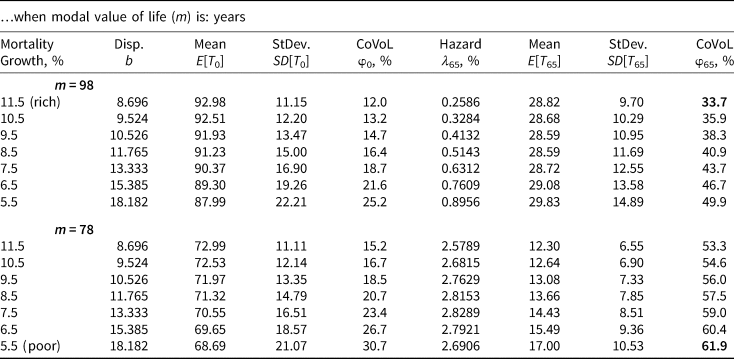
Table 4 offers a range of numerical values for the function: φ_x, at the age of x, under an assortment of parameter values for m (the mode of the Gompertz distribution) and b (the dispersion coefficient.) Note that by fixing (m, b) the hazard rate at any age x, is simply λ _x = (1/b)e ^(x−m)/b, as per the definition of the Gompertz mortality hazard rate.

Table 4. Coefficient of variation of longevity (CoVoL): φ_x

Note: These numbers (and ranges) are for illustrative purposes and based on theoretical Gompertz values and do not correspond to any specific income percentile or group. Note that the SD of longevity and the CoVoL are both higher when the mortality growth rate g increases.

For example, the values in the first row are computed assuming that m = 98 and the mortality growth rate is $1/b = 11.5\% $ per year, which implies that the dispersion coefficient is: b = 8.696 years. For reasons that should by now be obvious, I refer to this combination of (m, b) as rich (i.e., highest income percentile), and the life expectancy at birth: E[T ₀] = 92.98 years. The SD of the lifetime random variable at birth is: SD[T ₀] = 11.15 years, which is higher than the dispersion coefficient b = 8.696 by slightly more than 2 years. At birth, the SD: $SD\lsqb {T_0} \rsqb = b\,\pi /\sqrt 6 $, which is 28% greater than b.

To be clear, computing the mean and SD at birth under a Gompertz assumption for the evolution of the hazard rate λ _x, x = 0…ω, is somewhat artificial (or disingenuous). After all, even in the most developed countries mortality rates are relatively high in the first few years of life, reaching a minimum around the age of 10 and only starting to ‘behave’ in a Gompertz-like manner between the age of x = 30 to x = 95. I'm not saying all mortality tables at all ages are Gompertz. Rather, the point here in Table 4 is to provide some intuition for the moments of the Gompertz random variable as opposed to accurately modeling the earliest ages in the lifecycle. Needless to say, infants and children aren't purchasing life annuities or pooling longevity risk.

Moving along the first row of the table, the CoVoL is a mere $\varphi _0\lpar {98,\;8.686} \rpar = 12\% $ at birth, then increases over the lifecycle to reach $\varphi _{65}\lpar {98,\;8.696} \rpar = 33.7\% $ at the age of x = 65. Note – for the sake of replicability – that although they can in theory be derived analytically the CoVoL numbers at x ≫ 0 are computed numerically. The denominator of φ_x, that is the mean of the remaining lifetime, is available in closed form (see Appendix A.3 with r = 0), while the numerator requires a numerical procedure. In sum, the rich woman's CoVoL at the age of retirement age of x = 65 is $33.7\% $. Again, the m = 98 and b = 8.696 parameters are representative of the highest income percentiles in the Chetty et al. (Reference Chetty, Stepner, Abraham, Lin, Scuderi, Turner, Bergeron and Cutler2016) data. This 65-year-old has a mortality hazard rate of $\lambda _{65} = 0.2586\% $ at the age of x = 65.

Now, as I move down the rows within the first panel and artificially reduce the mortality growth rate from 11.5% to 5.5%, while holding the modal value of life fixed at 98 years, the CoVoL values increase. To be clear, holding m fixed and reducing g: = 1/b induces a corresponding increase in λ _x as per the sixth column in the table. Although these parameter combinations don't correspond to any particular income percentile the point here is to develop intuition for the link between age, parameters (m, b), hazard rates λ _x and CoVoL.

Notice how reducing the mortality growth rate (remember this is g = 1/b), that is increasing b, uniformly reduces the life expectancy at birth E[T ₀] and increases the SD[T ₀] at birth. The numerator goes up, the denominator goes down and so the CoVoL increases with higher values of b.

The situation becomes less obvious or clear-cut at the age of 65. Notice how the mean E[T ₆₅] starts-off at 28.82 years (when b = 8.696) and then declines as one would expect at higher values of b, but then flattens-out at 28.59 years and starts to increase. It seems the increased dispersion b then serves to increase the mean value, as often happens with highly skewed distributions. This is also driven by the fact the initial hazard rate at age 65 is higher. All in all, the SD[T ₆₅] does in fact increase monotonically with b and the net effect is that the coefficient of variation does in fact increase in b.

Moving from rich to poor, in the bottom panel of Table 4 in which the modal value of life is m = 78 years, the corresponding life expectancy values are (much) lower. The hazard rates are higher as well. At the very bottom row, where b = 18.182 years (i.e., the slowest aging), the life expectancy at retirement age x = 65 is now 17 years (vs. 28 years). The poor man's CoVoL is 61.9%, which is almost double the top row, compared to the rich woman's 33.7%.

The artificial numbers in Table 4 and the underlying intuition are quite important for understanding the comparative statics in the next section. Notice how the CoVoL is subtly affected by the interplay between age x, modal value m and dispersion value b. As x → m the CoVoL increases purely as a result of the underlying Gompertz law, even when b is unchanged. In other words, aging increases the relative riskiness of your remaining lifetime. From an economic point of view – as I will show in the next section – the demand for longevity insurance and risk pooling increases in age, a.k.a. with higher mortality rates. Just as importantly, fixing both x and m, and (only) increasing the value of b also increases CoVoL. At any given age x, your CoVoL is higher with higher m and/or with higher b. Figure 3 displays CoVoL numbers over the entire lifecycle for two sets of (m, b) parameters. Notice how it plateaus at higher ages and never exceeds 100%. One can think of it as the expected value of the Gompertz remaining lifetime: E[T _x] converging to SD[T _x], as x → ω. In probabilistic terms, at very advanced ages the amount of time you will actually live (yes, it's random) is very close to what you expect to live. See Figure 3.

Note: The y-axis (CoVoL) is defined as the ratio of the SD of expected lifetime SD[T _x] to mean lifetime E[T _x] at age x. The vertical line is at age x = 65, with exact values noted in Table 4. The Gompertz parameters are m = 98,  b = 8.696 (rich) and m = 78, b = 18.182 (poor.) Notice how both curves and the CoVoL converge to a value of φ = 1 at advanced ages independently of whether there is a mortality plateau.

Figure 3. The CoVoL over the lifecycle.

For clarity, the variability is unrelated to notions of stochastic mortality models, or aggregate changes in population q ₆₅ values over time. I am not using volatility to forecast mortality in (say) 50 years and the models in this paper are entirely deterministic. That said, if one graduates from a deterministic model of hazard rates λ _x, and postulates a stochastic model: $\tilde{\lambda} _x$, the φ_x metric would still be defined as the ratio of moments and should converge to a value of one at very advanced ages.

4.1 Pricing annuities

I use the symbol a(.) to denote the market price of a life annuity at age x. In words, paying a(.) to an insurance company or pension fund, obligates the issuer to return $\$ 1$ of income per year (or $\$ 1dt$ in continuous time) for the life of the buyer, a.k.a. retiree or annuitant. The items inside the bracket (.) are the conditional factors, which could be age, gender, health, etc. For example, a retiree might pay: a $\lpar {65} \rpar \, = \$ 20$ to purchase a life annuity providing $\$ 1$ per year for life starting at the age of x = 65, but the price might be a $\lpar {75} \rpar \, = \$ 14$ if purchased at age x = 70, etc. Both are completely arbitrary numbers, although throughout the paper for the sake of this discussion I'll assume life annuities scale and the price of $\$ 100,\!\!000$ of annual income is exactly $\$ 100,\!\!000$a(.). There are no bulk (economies of scale) discounts or (adverse selection-induced) penalties. Moreover, the only loading or frictions will come (implicitly) from being pooled with healthier and longer lived individuals, as opposed to profits or other institutional features. Now, in the above example market prices are differentiated by age x. In practice (most) companies and issuers differentiate by gender, while some go even further and underwrite annuities, that is price based on the health status of the annuitant. When needed, I will augment notation to include biological characteristics, namely the two Gompertz parameters (h _x, g) at the relevant age x.

Thus, a(h _x, g) denotes the market price of a $\$ 1$ per year life annuity, purchased at age x when the hazard rate is h = h _x, for an individual whose remaining lifetime random variable is modeled in Gompertz (h _x, g) space. These were all explained in Section 3. The point I make here is that these two bio-demographic characteristics are easily observable and can be used for underwriting in some jurisdictions, or at least for modeling purposes.

As far as finance and markets are concerned, interest rates (obviously) impact the price of pension and life annuities, so in the event I must draw attention to the underlying pricing rate: r, assuming it is constant, I will append a third parameter to the very beginning of the expression and write the annuity factor as: a(r, h, g) for completeness. Notice the absence of any age (x) in the expression, since this is already contained and included within the hazard rate (h _x). Occasionally the expression a(r, x, m, b) will make an appearance when I want to draw specific attention to the impact of a modal value (m) or global dispersion parameter (b), on the annuity valuation factor at an explicit age denoted by (x).

Notice that up to now I have only mentioned market prices as opposed to say theoretical model or economic values, which naturally might differ from each other. To link these two numbers, I refer to what actuaries might call the fundamental law of pricing mortality-contingent claims, or what financial economists might simply call No Arbitrage valuation. Either way, the market price: a(x) under a Gompertz law of mortality should be equal to the following value:

(4)$$a\lpar {r,h_x,g} \rpar \;: = \int\limits_0^{\omega -x} {e^{-rt}\,p\lpar {t,h_x,g} \rpar dt}, $$

where ω denotes the last possible age to which people are assumed to live and p(t, h _x, g) is the conditional (at age x and mortality rate h _x) survival probability. The underlying economic assumption is that if a large enough group of known (h _x, g)-types are pooled together they will – by the law of large numbers – eliminate any idiosyncratic mortality risk and the valuation is easily conducted by discounted cash-flow expectations. Another embedded assumption in equation (4) is that the interest rate is a constant r, although that really isn't critical. By assuming a constant rate r, equation (4) can be solved analytically using the Gamma function. See the technical appendix for more on this. Equation (4) is often used discretely, for example in Poterba et al. (Reference Poterba, Venti and Wise2011). From this point onward I will refrain from using market price or value and refer to a(.) as the annuity factor.

Before I proceed to the economics of the matter, it's important to focus attention on the sign of the partial derivatives of a(r, h _x, g), with respect to the three explicitly listed arguments. First, the annuity factor declines with increasing age and hazard rate h _x. Intuitively (and unlike a perpetuity) the cost of a constant $\$ 1$ of lifetime income declines as you get older (and closer to death). Likewise, the factor declines at higher valuation rates r, after all it's just a present value. Just as importantly, at any conditional age x and hazard rate h _x, the annuity factor declines as the growth rate g is increased, which is synonymous with individuals who have a lower remaining life horizon. These insights don't require much calculus and are discussed at greater length in the technical appendix.

Back to the economics of the matter. Let $\lpar {{\hat{h}}_x,\hat{g}} \rpar $ denote the Gompertz parameters that best fit population (group) mortality while $\lpar {h_x^i, g^i} \rpar $ denotes the parameters that best fit individual (sub-group) mortality. In particular, using ideas introduced in Section 3, I let $\lpar {h_x^1, g^1} \rpar $ denote the Gompertz parameters of individuals (i.e., sub-group) in the lowest income percentile, whereas $\lpar {h_x^{100}, g^{100}} \rpar $ denotes the Gompertz parameters of individuals in the highest income percentile. Therefore, the population modal and dispersion parameters would be the median values: $\hat{h} = h_x^{50}, $ and $\hat{g}_x = g^{50}$, respectively (albeit with a bit of hand waving).Footnote ⁶ As mentioned earlier, on the occasion that I want to draw attention to population averages for (m ⁱ) and (b ⁱ) parameters, I'll use the obvious: $\lpar {\hat{m}} \rpar $ and $\lpar {\hat{b}} \rpar $.

4.2 Measuring utility

Let U**(w) denote the value function (maximal utility) of the individual who annuitizes their wealth w, and U*(w) the value function of the individual who decides to self-insure (i.e., not own any annuities at all) and instead decides to fund retirement with a systematic withdrawal program, then:

(5)$$U^{{^\ast}{^\ast}}\lpar w \rpar \; \ge U^{^\ast}\lpar w \rpar.$$

This is the well-known result in annuity economics, noted and cited in Section 2. There exists a constant δ ≥ 0 such that:

(6)$$U^{{^\ast}{^\ast}}\lpar w \rpar \; = U^{^\ast}\lpar {w\lpar {1 + \delta} \rpar } \rpar.$$

A retiree who doesn't annuitize would require the δ percent increase in their wealth w to induce the same level of utility as someone who does annuitize. Given that we are operating with constant relative risk aversion (CRRA) utility and no pre-existing annuity income, I will set w = 1 and refer to the AEW by (1 + δ), and the value of longevity risk pooling by δ. To close the loop on all these (utility based) definitions, note that if my subjective value of risk pooling is: $\delta = 25\% $, and the AEW is $\$ 1.25$, then someone with $w = \$ 125$ of initial wealth would be willing to pay $\$ 25$ or $100δ/(1 + δ) to have access to the annuity. The WtP is then δ/(1 + δ).

Whether it be AEW, WtP or simply the value of pooling δ, all essentially measure the same thing and will be used interchangeably in the paper, unless the numbers themselves are important. Either way, the δ is a function of the individual Gompertz parameters $\lpar {h_x^i, g^i} \rpar $, the market pricing parameters $\lpar {{\hat{h}}_x,\hat{g}} \rpar $, and the utility-based preferences involving risk γ and discounting ρ = r.

Moving on, assume an individual (denoted by i) and their force of mortality are individually Gompertz parameters and the population is also (approximated as) Gompertz, upon which annuity factors are based. The individual's AEW can be expressed as:

(7)$$1 + \delta _x^i = \displaystyle{{a{(r,x,m^i,b^i)}^{1/\lpar {1-\gamma} \rpar }a{(r,x,\hat{m},\hat{b})}^{-1}} \over {a{(r,x-b^i\,\ln {\rm [}\gamma {\rm ]},m^i,b^i)}^{\gamma /\lpar {1-\gamma} \rpar }}} = \displaystyle{{a{(r,h_x^i, g^i,)}^{1/\lpar {1-\gamma} \rpar }a{(r,{\hat{h}}_x,\hat{g})}^{-1}} \over {a{(r,h_x^i /\gamma, g^i)}^{\gamma /\lpar {1-\gamma} \rpar }}}$$

where γ denotes the coefficient of relative risk aversion within CRRA utility, and assuming the subjective discount rate is (also) equal to r.

I have deliberately expressed the annuity factor using both (m, b) and (h _x, g) formulations, mainly so that δ can be (easily) computed when either set of parameters are available. Note that when annuity prices are fair (i.e., pooling with equal risks) the value of $h_x^i = \hat{h}_x$, and as well the value of $g_i = \hat{g}$. So, the expression in equation (7) can be simplified further, which I will do in a moment.

The value of longevity risk pooling δ is an increasing function of the CoVoL for the individual. The precise mechanism by which this operates is via the higher mortality hazard rate h _x. To be clear, even if g is held constant, a higher value of h _x induces a higher (CoVoL and) value of δ. This, again, is when annuities are fairly priced so that $h_x = \hat{h}_x$ and $g = \hat{g}$ in equation (7). Supporting proofs and comparative statics are presented in the technical appendix. I also refer to Milevsky and Huang (Reference Milevsky and Huang2018) for additional supporting material. Note that my interest in this paper is to use the expression for AEW, a.k.a. (1 + δ) not to derive it, which is fully developed in Milevsky and Huang (Reference Milevsky and Huang2018).

Finally, in the homogeneous case everyone in the sub-group experiences the exact same Gompertz force of mortality, that is $h_x = \hat{h}_x$ and $g = \hat{g}$. The AEW is:

(8)$$1 + \delta _x = \left( {\displaystyle{{a\lpar {r,x,m,b} \rpar } \over {a\lpar {r,x-\hat{b}\,{\rm ln}\,\gamma, m,b} \rpar }}} \right)^{\gamma /(1-\gamma )} = \left( {\displaystyle{{a\lpar {r,h_x,g} \rpar } \over {a\lpar {r,h_x/\gamma, g} \rpar }}} \right)^{\gamma /(1-\gamma )}.$$

It is a simple function of the ratio of two actuarial annuity factors and easily computed in either discrete or continuous form.

In particular, notice that the respective annuity factors in equation (8) are computed at two distinct ages (or hazard rates). The numerator is computed at the BA: x (or hazard rate h _x), and the denominator is computed at a modified (risk-adjusted) age: $x-\hat{b}\,\ln \,\gamma $ (or hazard rate h _x/γ). The modified age in the denominator's factor is under (younger than) x whenever γ > 1. The lower modified age increases the annuity factor and the AEW. Nevertheless, even when γ < 1, the value of δ _x > 0 provided γ > 0. Here are some numerical examples and intuition for the AEW.

4.3 A simple numerical example: two hypothetical groups

Assume the remaining life expectancy at the age of 65 of a hypothetically constructed Group A is 11.95 years and the underlying Gompertz mortality parameters are m = 75.02 and b = 11.87. The CoVoL at age 65 is $60.4\% $. Now, assume the remaining life expectancy for a hypothetical Group B is: E[T ₆₅] = 23.64 years and Gompertz parameters are m = 91.72 and b = 12.87, for a CoVoL of $47.4\% $. As this is only a numerical example, I'll assume that the (subjective discount rate and) valuation rate are $r = 3\% $, and the coefficient of relative risk aversion is γ = 3 in the CRRA utility.

Under these parameter values a representative Group A (65 year old, retiree) would value the longevity insurance at $\delta = 89.32\% $ if they could pool this risk with other similar Group A members, by acquiring fairly priced life annuities based on their own population: m = 75.02 and b = 11.87 parameters. This AEW is in line with the (generally) large benefits from annuitization reported in (many) other studies over the last 30 years, noted in the literature review of Section 2.

Now, let's examine the representative Group B retiree, assuming the same $r = 3\% $ valuation rate and γ = 3, coefficient of risk aversion. If they are pooled with homogeneous risks from Group B, their δ value at the age of x = 65 is lower than their Group A counterparts. Intuitively, their CoVoL is also lower at age 65. In particular, using the m = 91.72, b = 12.87 values, equation (8) leads to a value of $\delta = 48.39\% $ which is lower than what a Group A member would be willing to pay. Indeed, what drives the δ for (fair) longevity insurance is the volatility of longevity (via the m and b) and not the demographic fact that the Group B retirees live longer.

Moving on to a larger heterogeneous pool, imagine Group A and Group B, both at CA 65, are mixed together in equal amounts. To keep the system fair, the pension annuities are priced based on the mixed population mortality. With a bit of hand waving, assume the resulting Gompertz parameters upon which the group annuities are priced are m = 85.45 and b = 12.41. Intuitively, the Group A member is presented with a relatively worse annuity price and the Group B member is getting a relatively better price.

This assumes both groups are forced to purchase annuities at the same price in a compulsory system. The AEW is based on the group population (for market pricing) and individual (for lifecycle utility) mortality. See equation (7). The group annuity factor – or price they both pay – is now a $\lpar {r = 3\%, \;65,\;\hat{m} = 85.45,\;\hat{b} = 12.41} \rpar = 13.583$, which isn't actuarially fair to either of them. It's advantageous to the Group B member (who would have had to pay 15.97) and disadvantageous to the Group A member (who would only have to pay 9.493).

Here is the main point. The Group B member now experiences: δ = 74.48, which is higher than the prior (homogeneous case of): $\delta = 48.39\% $. In contrast, the Group A member is faced with loaded prices (13.583 vs. 9.493) and they are only valuing the annuity at $\delta = 32.32\% $. In fact, if the Group A member had a life expectancy that was (even) lower, but still paid the same group price, it's conceivable the δ in equation (7) might actually be negative. They would rather take their chances and self-insure longevity.

Figure 4 illustrates this relationship graphically over a spectrum of possible m values. On the left are individuals (think Group A) with low life expectancy (proxied by m) values and a correspondingly higher volatility of longevity at retirement. To the right are individuals (think Group B) with higher life expectancy and lower volatility of longevity. The Gompertz dispersion of longevity – in contrast to the volatility of longevity – for the purposes of computing equation (7), is held constant at 1/g = b = 12 years. The upper range is based on γ = 5, that is higher levels of risk aversion, whereas the lower range is for γ = 1, albeit with slight modifications in equation (7) to account for logarithmic utility.

Note: Figure is based on a valuation rate r = 3% and coefficient of relative risk aversion from γ = 5 (top) to γ = 1 (bottom). When annuities are priced based on individual mortality (m _i, b = 12), the value of AEW declines in m _i. But when annuities are priced based on group mortality $\lpar {\hat{m},b = 12} \rpar $, the value of AEW increases in m _i, due to the implicit loading.

Figure 4. AEW under a range of values for m.

Notice that as m increases, the value of longevity risk pooling and WtP declines – when the pooling is homogeneous. A Group B retiree (paying fair prices) experiences a δ that is lower than a Group A (paying fair prices); but when they are mixed together and both pay the same group price, the curve is reversed. Intrinsically the Group A values longevity insurance more, due to his/her higher volatility of longevity, but the positive loading reduces its appeal. In contrast, the Group B member who is now willing to pay more for a relatively cheap life annuity. With that intuition out of the way, we can back to our main empirical question. What happens in the USA across different income percentiles?