


1. Introduction
Our concern is with the development of streamwise vortex instabilities caused by wall roughness in growing boundary layers. The instability we investigate here is a direct consequence of wall waviness; we are not concerned with the effect of wall waviness on Tollmien–Schlichting waves or crossflow vortices. The reader interested in those problems is referred to, for example, Wie & Malik (Reference Wie and Malik1998) and Thomas et al. (Reference Thomas, Mughal, Gipon, Ashworth and Martinez-Cava2016). For definiteness, we will focus on Falkner–Skan boundary layers and, following Gajjar & Hall (Reference Gajjar and Hall2020), Hall (Reference Hall2020, Reference Hall2021) and Hall & Ozcakir (Reference Hall and Ozcakir2021), wall roughness is modelled by small amplitude wall undulations in the streamwise direction.
In pipes and channels motivation to investigate the effect of wall undulations comes from the heat transfer community where wavy walls have long been used as an aid to mixing; see, for example, Gschwind, Regele & Kottke (Reference Gschwind, Regele and Kottke1995), Kandlikar (Reference Kandlikar2008), Ligrani, Oliveira & Blaskovich (Reference Ligrani, Oliveira and Blaskovich2003) and Nishimura, Yoshino & Kawamura (Reference Nishimura, Yoshino and Kawamura1987). Often these devices operate at Reynolds numbers where turbulence in smooth channels or pipes occurs; therefore, there is a strong interest in the question of how wall undulations influence transition to turbulence in such shear flows. We note here that our concern is with instabilities caused by roughness rather than the receptivity problem where roughness is the enabler of instabilities present in the absence of roughness; see, for example, Ruban (Reference Ruban1984), Goldstein (Reference Goldstein1985) and Hall (Reference Hall1990).
Instabilities of the flows in pipes of radii varying periodically in the streamwise direction have been considered by Cotrell, McFadden & Alder (Reference Cotrell, McFadden and Alder2008) and Loh & Blackburn (Reference Loh and Blackburn2011). It was found that wall waviness can destabilise the flows through what was described as a centrifugal instability mechanism. More recent work by Hall (Reference Hall2020, Reference Hall2021) and Hall & Ozcakir (Reference Hall and Ozcakir2021) shows that the instability mechanism is in fact of the vortex-wave interaction type facilitated by wall waviness rather than finite amplitude effects. Cotrell et al. (Reference Cotrell, McFadden and Alder2008) focused on axisymmetric disturbances but reported that non-axisymmetric modes were more stable, however, Loh & Blackburn (Reference Loh and Blackburn2011) found that non-axisymmetric modes were the first to become unstable. Hall & Ozcakir (Reference Hall and Ozcakir2021) considered both two- and three-dimensional roughness in the form of surface undulations in both the streamwise and azimuthal directions and, like the case with Loh & Blackburn (Reference Loh and Blackburn2011), found that the two-dimensional case is more unstable.
Related problems in channel flow of periodically varying widths have been considered by Floryan (Reference Floryan2002, Reference Floryan2003, Reference Floryan2015) using large-scale global instability computations of the linearized Navier–Stokes equations. Recently Hall (Reference Hall2020) has shown how the small amplitude case, which is in fact the case of most practical interest, can be described by a variant of vortex-wave interaction theory. Henceforth, we refer to the latter as VWI theory. Hall (Reference Hall2020) used the theory to predict the critical Reynolds number for fully developed flows in channels with walls having small amplitude undulations. Here we will extend that theory to growing boundary layer flows. The mechanism uncovered in Hall (Reference Hall2020) is operational whenever a shear flow interacts with a wavy wall and so it is relevant to both internal and external flows, but various modifications are needed to allow for the change in geometry. For channels with walls having wall undulations of wavelength slowly varying in the streamwise direction, Gajjar & Hall (Reference Gajjar and Hall2020) showed that the disturbance equations reduce to a spatially modulated form of the Görtler vortex equations. In the regime considered by Gajjar & Hall (Reference Gajjar and Hall2020) the VWI mechanism is not operational and the instability in that case is centrifugal in origin. Floquet theory was used in the latter paper to show that both subharmonic and synchronous instabilities are possible. Hall (Reference Hall2021) investigated the Görter vortex mechanism at long wavelengths and gave limited results for roughness instabilities in that limit for Blasius flow. As part of the present investigation, we extend the latter long wavelength results to Falkner–Skan flows and consider all wavenumber regimes.
In VWI theory streamwise vortices are sustained by wave–wave interactions in the critical layer associated with the wave. The wave exists as a neutral disturbance of the streaky part of the flow; see Hall & Smith (Reference Hall and Smith1989), Hall & Smith (Reference Hall and Smith1991), Hall & Sherwin (Reference Hall and Sherwin2010), Deguchi & Hall (Reference Deguchi and Hall2014) and Hall (Reference Hall2018). The linear instability mechanism uncovered by Hall (Reference Hall2020) replaces the wave–wave interaction of a disturbance of the shear flow within VWI by an interaction between the wavy mean flow corrections produced by the wall undulations and the streamwise vortex. Thus, the mechanism of Hall (Reference Hall2020) is a hybrid form of VWI. An alternative derivation of what was exactly the VWI theory description of exact coherent structures had been uncovered numerically by Nagata (Reference Nagata1990) and subsequently Waleffe and colleagues who described it as a ‘self-sustained process’; see, for example, Waleffe (Reference Waleffe2001) and Wang, Gibson & Waleffe (Reference Wang, Gibson and Waleffe2007).
In the mechanism given by Hall (Reference Hall2020) a streamwise vortex consisting of an  $O(1)$ streamwise velocity component, which we refer to as the streak, and a smaller roll flow in the spanwise and normal directions are driven by interactions caused by the wall waviness. In the absence of roughness or curvature, the roll and streak equations are decoupled, but in the presence of roughness a boundary condition links the shear at the wall of the roll and streak. Here we will generalize the fully developed case considered by Hall (Reference Hall2020) to growing boundary layers. The instability, though not of centrifugal type, satisfies the linear Görtler vortex equations of Hall (Reference Hall1983) with zero Görtler number and a stress boundary condition replacing the no-slip condition on the spanwise roll velocity at the wall. Not surprisingly the instability will be seen to have some similarities with Görtler vortices. It should be noted that in some shear flows where the roughness instability considered here is operational Tollmien–Schlichting or other instabilities might be more unstable, on the other hand in Hagen–Poiseuille flow or Couette flow no alternative linear instability is present.
Streamwise vortex instabilities in boundary layers over curved walls are referred to as Görtler vortices following the work of Görtler (Reference Görtler1940). The instability grows more slowly than Tollmien–Schlichting waves or crossflow vortices, indeed it grows on the same length scale as the unperturbed flow, and must be described using a non-parallel theory. For that reason, attempts to describe Görtler vortices by a quasi-parallel flow approximation produced inconsistent and what turned out to be physically unrealistic results; see, for example, Smith (Reference Smith1955) or, for a comprehensive review of the parallel flow work, Floryan (Reference Floryan1991). The issues associated with the parallel flow theories in both the linear and nonlinear regimes were resolved by Hall (Reference Hall1982, Reference Hall1983, Reference Hall1988, Reference Hall1990) and Hall & Lakin (Reference Hall and Lakin1988). It was shown that the instability equations cannot be reduced in a quasi-parallel manner unless the Görtler number is large. Therefore, the instability problem must be solved by marching in the streamwise direction. Thus, Hall (Reference Hall1982), Denier, Hall & Seddougui (Reference Denier, Hall and Seddougui1991) and Choudhari, Hall & Street (Reference Choudhari, Hall and Street1994) gave a comprehensive description of the different regimes at high Görtler numbers. More recently, Wu, Zhao & Luo (Reference Wu, Zhao and Luo2011) repeated the analysis of Hall (Reference Hall2021) using the streamwise coordinate as the large parameter but, as pointed out in Hall (Reference Hall2021), overlooked the most unstable mode in the left-hand branch regime. Some preliminary observations on the long wavelength roughness instability for Blasius flow are given in Hall (Reference Hall2021). Henceforth, we will refer to the papers Denier et al. (Reference Denier, Hall and Seddougui1991) and Choudhari et al. (Reference Choudhari, Hall and Street1994) as DHS and CHS, respectively, and refer to Hall (Reference Hall2020) as H1. We will refer to the small and large wavenumber branches at large values of the roughness parameter as the left- and right-hand branches.
Our analysis will show that the small wavenumber regime where the flow develops in a non-parallel manner selects the disturbance generated downstream. We show that, for some Falkner–Skan flows, a disturbance imposed sufficiently close to the leading edge grows algebraically before roughness comes into play and converts that growth into more explosive exponential growth. If the initial development is for a flow where only decaying algebraic solutions are possible, the least stable such solution is selected and once again roughness then stops that decays and ultimately produces exponential growth. We show that, for a Falkner–Skan flow with free stream varying like  $X^n$, where
  $X$ denotes scaled downstream distance, the exponential growth is like
  $\exp ({dX^{({(3n+1)}/{2})}})$, where
  $d$ is a constant. Thus, for stagnation point flow, the argument of the exponential is proportional to
  $X^2$ and the growth is unusually rapid. We will show that Falkner–Skan flows corresponding to
  $90^{\circ }$ wedges are uniquely susceptible to the roughness mechanism and lead to indefinite exponential growth at the largest rate available. By way of contrast, the flows past wedges of angles less than
  $90^{\circ }$ are unstable for only a finite downstream extent. Wedges of an angle greater than
  $90^{\circ }$ remain unstable indefinitely as
  $X$ increases but do not grow at the fastest rate possible at a given high value of the roughness amplitude.
The procedure adopted in the remainder of the paper is as follows. In § 2 we will formulate the roughness-induced instability problem for a two-dimensional boundary layer over a wavy wall. In § 3 we will solve the instability equations for asymptotic suction flow. The asymptotic structure uncovered there is then used as a framework to investigate growing boundary layers in § 4. In § 5 we will discuss numerical solutions of the roughness instability equations at  $O(1)$ values of the roughness parameter. In § 6 we will use the theory to predict universally valid results concerning roughness instabilities in shear flows. In § 6 we also briefly describe how the model used to represent roughness can be made more realistic. In § 7 we draw some conclusions and show how the instability mechanism discussed relates to instabilities of triple-deck flows. In an appendix we briefly describe how the structure discussed in CHS can be adapted to the present problem to give the link between the small and
  $O(1)$ wavenumber regimes.
2. The disturbance equations for roughness-induced instability
Consider the viscous incompressible flow of a fluid with viscosity  $\nu$ over the semi-infinite flat plate
  $x^*>0,\ y^*=0$. We take
  $L$ as a typical length scale in the
  $x^*$ direction so that if the free-stream speed is
  $U_0u_e({x^*}/{L})$ the boundary layer thickness is
  $\varDelta =\sqrt {{\nu L}/{U_0}}$. We define a Reynolds number based on the boundary layer thickness by
 \begin{equation} {\textit{Re}}=\frac{U_0\varDelta}{\nu}=\sqrt{\frac{U L}{\nu}}=\sqrt{R}. \end{equation}
Using  $\varDelta$ as the length scale we define
  $(x,y,z)=(x^*, y^*, z^*)/\varDelta$, and taking
  $U_0$ as a typical velocity we define
  $(u,v,w)=(u^*, v^*, w^*) /U_0$. If we then define the scaled pressure
  $p=p^*/\rho U_0^2$, where
  $\rho$ is the density, then the steady momentum and continuity equations take the form
 $$\begin{gather} [{\boldsymbol{u}}\boldsymbol{\cdot}\boldsymbol{\nabla}]{\boldsymbol{u}} ={-}\boldsymbol{\nabla}{p}+\frac{1}{Re}\nabla^{2}{\boldsymbol{u}}, \end{gather}$$
 $$\begin{gather}\boldsymbol{\nabla}\boldsymbol{\cdot} \boldsymbol{u} =0, \end{gather}$$
where  $\boldsymbol {\nabla }=({\partial }/{\partial x},{\partial }/{\partial y},{\partial }/{\partial z})$. We restrict our attention to the high-Reynolds-number limit so that the leading order approximation to the equations of motion in the boundary layer, i.e. the region
  $y=O(1),\ X={x}/{Re}=O(1)$, is given by
 $$\begin{gather} {\boldsymbol{u}}={\boldsymbol{u}}_b=\left({\bar{u}}(X,y),\ \frac{1}{Re}\bar{v}(X,y),0\right)+\cdots, \end{gather}$$
 $$\begin{gather}p= {p}_b ={-}\frac{{u_e}^2}{2} +\cdots, \end{gather}$$
where  $(\bar {u}, \bar {v})$ satisfies the boundary layer equations
 $$\begin{gather} \bar{u}\bar{u}_X+\bar{v}\bar{u}_y =u_eu_{eX}+\bar{u}_{yy}, \end{gather}$$
 $$\begin{gather}\bar{u}_X+\bar{v}_y =0, \end{gather}$$
subject to the conditions
 \begin{equation} \bar{u}=\bar{v}=0,\quad y=0,\quad \bar{u} \rightarrow u_e,\quad y \rightarrow \infty. \end{equation}
Now we perturb the above flow to a steady streamwise vortex disturbance of size  $\delta \ll 1$. We assume the vortex is periodic in the spanwise direction with wavelength scaled on the boundary layer thickness and write
 $$\begin{gather} {\boldsymbol{u}} ={\boldsymbol{u}}_b+\delta\left(U(X,y)\cos kz, \frac{V(X,y)}{Re}\cos kz, \frac{W(X,y)}{Re}\sin kz\right), \end{gather}$$
 $$\begin{gather}p=p_b+\delta\frac{P(X,y)}{Re^2}\cos kz. \end{gather}$$
The relative scalings of the perturbation velocity components are the usual ones for Taylor–Görtler vortices as first indicated by Taylor (Reference Taylor1923). Substituting into the equations of motion and linearizing with respect to the vortex amplitude  $\delta$, we find that the perturbation equations are
 $$\begin{gather} \bar{u}U_X+\bar{v}U_y+U\overline{u}_X+ {V}\overline{u}_y=U_{yy}-k^2U, \end{gather}$$
 $$\begin{gather}\bar{u}V_X+\bar{v}V_y+U\overline{v}_X+ {V}\overline{v}_y={-}P_y+V_{yy}-k^2V, \end{gather}$$
 $$\begin{gather}\bar{u}W_X+\bar{v}W_y=kP+W_{yy}-k^2W, \end{gather}$$
 $$\begin{gather}U_X+V_y+kW =0. \end{gather}$$
In the absence of destabilising effects due to wall curvature all perturbations inserted into the flow at some location will ultimately decay, though long wavelength perturbations inserted close to the leading edge can initially undergo weak algebraic growth; see Bassom & Hall (Reference Bassom and Hall1993) and Luchini (Reference Luchini1996). If the wall is curved then a term proportional to  $\bar {u}U$ is inserted into the left-hand side of (2.12). That term provides a coupling between (2.11) and (2.12)–(2.13), thus enabling a centrifugal instability to occur in some boundary layers; see Hall (Reference Hall1983).
The destabilisation due to wall undulations couples (2.12)–(2.13) to (2.11) through the boundary conditions at the wall. The analysis of H1 was for fully developed flow in a channel and so must be adapted to deal with a spatially evolving mean flow. The mechanism which produces the coupling is a hybrid form of VWI theory as described by Hall & Smith (Reference Hall and Smith1991) and Hall & Sherwin (Reference Hall and Sherwin2010). The mechanism is crucially dependent on the roll part of the vortex being of size  ${1}/{Re}$ smaller than the streamwise component which we will refer to as the streak.
Before writing down the appropriate modifications of (2.9) and (2.10) to take account of the undulating wall we explain the mechanism which will lead to the instability. As mentioned above, the key to understanding the origin of the instability is the fact that at high values of  $Re$ the roll part of a streamwise vortex is small compared with the streak part, and that imbalance is exactly the same for the mean state
  ${\boldsymbol {u}}_b$. The upshot of this is that in the viscous wall layer where
  $u_b$ and the streak part of the streamwise vortex adjust to satisfy no-slip on the undulating wall, the normal and spanwise velocity components of the corrections caused by the waviness are bigger than the corrections associated with
  $v_b$ and the roll part of the vortex. An examination of the nonlinear terms in the spanwise momentum equation averaged over the wavelength of the wall fixes the size of
  $\epsilon$ which enables the spanwise component of the roll to be driven at leading order by the interaction of the
  $X$ dependent basic and vortex flows in the
  $y$–
$y$– $z$ plane. Thus, the Reynolds stresses associated with the flow driven by the wall waviness induce a streamwise vortex flow. This is of course just the steady-streaming effect well known in the context of time periodic flows; see, for example, Stuart (Reference Stuart1966).
Suppose that the undulating wall has wavenumber  $\alpha$ and amplitude
  $\epsilon$ and so is defined by
 \begin{equation} y=2\epsilon \cos \alpha x. \end{equation}
Note here that the wall shape is a function of the fast variable  $x$ rather than
  $X$, thus, we have taken the wall wavelength to be comparable to the boundary layer depth rather than
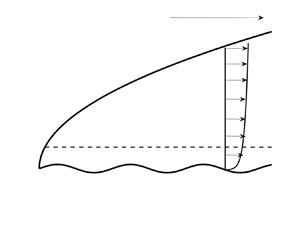
  $L.$ Because the wall varies on the boundary layer scale in the streamwise direction, the adjustment of the flow given by (2.9) and (2.10) to account for the undulating wall requires a viscous layer where
  $({1}/{Re})({\partial ^2}/{\partial y^2})\sim u_b({\partial }/{\partial x})$ so that it is of thickness
  $Re^{-({1}/{3})}$, and we assume that this is large compared with
  $\epsilon$ the amplitude of the wall waviness; see figure 1. We define a wall layer variable
  $\eta =Re^{{1}/{3}}y$ and expand the streamwise velocity component in the wall layer in the form
 \begin{align} u &= Re^{-({1}/{3})} \eta[\lambda+\mu \delta \cos kz]+\cdots +\epsilon (u_1(X,\eta)E+\textrm{c.c.} \nonumber\\ &\quad +\delta [U_1(X,\eta) E+\textrm{c.c.}]\cos kz)+\cdots. \end{align}
Here we have defined  $E=\textrm {e}^{\textrm {i}\alpha x}$, c.c. denotes complex conjugate and
  $\lambda =\overline {u}_{y}(X,0), \mu =U_{y}(X,0)$ are the shears of the basic boundary layer and streak at the wall. The terms proportional to
  $\epsilon$ are needed so as to satisfy the no-slip condition at the undulating wall. Note that the above expansion is only valid if
  $\epsilon << Re^{-({1}/{3})}$ and if
  $\epsilon$ is increased until
  $\epsilon \sim Re^{-({1}/{3})}$ the flow in the wall layer and the main part of the boundary layer couple and cannot be solved for independently, this type of interactive regime is discussed in Smith (Reference Smith1982). In the wall layer
  ${\partial }/{\partial x}\sim {\partial }/{\partial z}\sim O(1),\ {\partial }/{\partial y}=O(Re^{1/3})$ so that the expansion of
  $v$ in the wall layer takes the form
 \begin{align} v &= O( Re^{-({5}/{3})}) +\cdots +{\epsilon}Re^{-({1}/{3})} ( v_1(X,\eta)E+ \textrm{c.c.}\nonumber\\ &\quad +\delta [V_1(X,\eta) E+\textrm{c.c.}]\cos kz )+\cdots. \end{align}
The first term above corresponds to the local expansion of the  $y$ component of the unperturbed boundary layer in the wall layer whilst the second and third terms are driven by the
  $O(\epsilon )$ terms in (2.16). The expansion of
  $w$ is
 \begin{equation} w= {\epsilon} [ \delta W_1(X,\eta) E+\textrm{c.c.}+ ]\sin kz+\delta \epsilon^2 Re^{1/3}{\mathcal{W}}( X,\eta)\sin kz+\cdots. \end{equation}
The order  $\epsilon$ term once again has its size fixed by the
  $O(\epsilon )$ term in the streamwise velocity through the continuity equation. The last term arises from the nonlinear interaction of the order
  $\epsilon$ terms in the velocity field and we will fix
  $\epsilon$ by making the term of the same size as the spanwise component of the roll outside the wall layer. Note that the last term depends on the slow variable
  $X$ rather than the faster streamwise variable. Finally, we write down the expansion of the pressure
 \begin{equation} p={-}\frac{{u_e}^2}{2}+ \cdots {\epsilon}Re^{-({1}/{3})} ( p_1(X,\eta)E+\textrm{c.c.}+\delta [P_1(X,\eta) E+\textrm{c.c.}]\cos kz )+\cdots. \end{equation}
Substituting the above expansions of  $u,v,w,p$ into the equations of motion in the wall layer, we find the following leading order problem to determine
  $u_1, v_1, p_1$:
 $$\begin{gather} \textrm{i}\alpha \lambda u_1\eta+\lambda v_1={-}\textrm{i}\alpha p_1 +u_{1\eta \eta}, \end{gather}$$
 $$\begin{gather}p_{1\eta}=0, \end{gather}$$
 $$\begin{gather}\textrm{i}\alpha u_1+v_{1\eta}=0, \end{gather}$$
which is to be solved subject to
 \begin{equation} u_1={-}\lambda,\quad v_1=0,\quad \eta=0,\quad u_1\rightarrow 0,\quad \eta \rightarrow \infty. \end{equation}
The condition on  $u_1$ when
  $\eta \rightarrow \infty$ is necessitated by the corresponding inviscid problem for
  $y=O(1)$ which has no solution with the normal velocity vanishing at the wall. The required solution is given by
 \begin{equation} v_1={-}3 \gamma^{2/3}\int_0^\xi \textrm{d}\phi\int_\infty^\phi Ai(\theta)\,\textrm{d}\theta. \end{equation}
Here  $\gamma =\textrm {i}\alpha \lambda$,
  $Ai$ is the Airy function, and the variable
  $\xi$ is defined by
  $\xi =\gamma ^{1/3}\eta$. We deduce from the above equation that
 \begin{equation} v_1\rightarrow -3 \gamma^{2/3} Ai'(0),\quad \xi \rightarrow \infty. \end{equation}
The leading-order approximation to the terms proportional to  $\delta \epsilon$ in the equations of motion in the wall layer gives
 $$\begin{gather} \textrm{i}\alpha \lambda U_1\eta+\lambda V_1+\textrm{i} \alpha \mu \eta u_1+v_1\mu={-}\textrm{i} \alpha P_1 +U_{1\eta \eta}, \end{gather}$$
 $$\begin{gather}P_{1\eta}=0, \end{gather}$$
 $$\begin{gather}\textrm{i}\alpha \lambda W_1\eta =k P_1 +W_{1\eta \eta}, \end{gather}$$
 $$\begin{gather}\textrm{i}\alpha U_1+V_{1\eta}+kW_1=0, \end{gather}$$
which are to be solved subject to
 \begin{equation} U_1={-}\mu,\quad V_1=0,\quad \eta=0,\quad U_1, \rightarrow 0,\quad \eta \rightarrow \infty. \end{equation}
The condition on  $U_1$ at
  $\infty$ arises because
  $V_{1\xi }$ must tend to zero at infinity because the corresponding motion induced in the main part of the boundary layer is inviscid and cannot have its normal velocity reduced to zero as the wall is approached. That is because the boundary layer is inviscidly stable to travelling wave perturbations on the boundary layer length scale. In order to solve (2.26)–(2.29), we multiply (2.26) and (2.28) by
  $\textrm {i}\alpha$ and
  $k$, respectively, and add before eliminating
  $[\textrm {i} \alpha U_1 +kW_1]$ using (2.29). If we then eliminate
  $P_1$ by differentiating with respect to
  $\eta$ we find that, written in terms of
  $\xi$,
  $V_{1\xi \xi }$ satisfies the Airy equation. The required solution for
  $V_1$ has
 \begin{equation} V_{1\xi}={-}\frac{3\mu \gamma^{2/3}}{\lambda}\int_\infty^\xi Ai(\theta)\,\textrm{d}\theta -\frac{\mu \gamma^{2/3}}{\lambda}Ai''(\xi). \end{equation}
If  $W_1$ is not to grow exponentially for large
  $\xi$, we can then solve the spanwise momentum equation to give
 \begin{equation} W_1={-}k\gamma^{-({2}/{3})} P_1{\mathcal{L}}(\xi), \end{equation}
where the Scorer function  $\mathcal {L}$ satisfies
  ${\mathcal {L}}''-\xi {\mathcal {L}}=1,$ with
  ${\mathcal {L}}(0)={\mathcal {L}}(\infty )=0$. The corresponding pressure field is found by combining (2.26) and (2.28), setting
  $\xi =0$ to give
 \begin{align} (\alpha^2+k^2)P_1 &={-}\gamma^{2/3}(i\alpha U_1+k W_1)_{\xi\xi}(X,\xi=0)= {\gamma } V_{1\xi\xi\xi}(X,\xi=0) \nonumber\\ &={-}\frac{5\mu \gamma^{5/3}Ai'(0)} {\lambda }. \end{align}
It follows from (2.31) and the  $z$ momentum equation that
 \begin{equation} V_1 \rightarrow -2 {\mu} \lambda^{{-}1} \gamma^{2/3} Ai'(0),\quad W_1\sim{-}\frac{5k\mu\gamma^{2/3} Ai'(0)}{\eta\lambda[\alpha^2+k^2]},\quad \eta \rightarrow \infty. \end{equation}
Now consider the integral  $I$ given below and integrate by parts and use continuity to give
 \begin{equation} I=\int_0^{{{2 {\rm \pi}}/{\alpha}}}(uw_x+vw_y+ww_z)\,{\textrm{d}x}= \int_0^{{{2 {\rm \pi}}/{\alpha}}}([vw]_y+2ww_z)\,{\textrm{d}x}+\cdots. \end{equation}
Here the terms denoted by  $\cdots$ are present because the integrand depends on both the fast
  $x$ variable and the slow variable
  $X$. It follows from the above result together with (2.16)–(2.18) that
 \begin{equation} \frac{\partial^2{\mathcal{W}}}{\partial \eta^2}=v_1\bar{W}_{1\eta}+\textrm{c.c.} \end{equation}
where an overbar denotes the complex conjugate. For large values of  $\eta$, we then see using (2.34a,b) that
 \begin{equation} \frac{\partial^2{\mathcal{W}}}{\partial \eta^2}\simeq{-}\frac{30 Ai'^2(0) \lambda^{1/3}\alpha^{4/3}k\mu}{\eta^2[\alpha^2+k^2]}. \end{equation}
Integrating twice with respect to  $\eta$ and writing the leading-order term in terms of
  $y$ rather than
  $\eta$ we obtain
 \begin{equation} {\mathcal{W}}\rightarrow \frac{10\alpha^{4/3}\lambda^{1/3}k\mu Ai'^2(0)}{\alpha^2+k^2} [\log{Re}+3{\log y} ]+\cdots, \quad \eta \rightarrow \infty. \end{equation}
Neglecting the term proportional to  $\log y$, the above provides an inner boundary condition for the spanwise velocity component of a roll flow in the main part of the boundary layer. The latter roll flow will be of the same size as the assumed roll flow in the main boundary layer in (2.9) if we choose
  $\epsilon$ appropriately. More precisely, if we define an
  $O(1)$ parameter
  $\kappa$ by
 \begin{equation} \epsilon^2\log Re=\frac{\kappa}{Re^{4/3}}, \end{equation}
and note that  $\mu =U_y(X,0)$, then (2.38) implies that the vortex equations (2.11)–(2.14) must be solved subject to
 $$\begin{gather} U, V, W, \rightarrow 0,\quad y\rightarrow \infty, \end{gather}$$
 $$\begin{gather}U=V=0,\quad W=\frac{10\kappa\alpha^{4/3}\lambda^{1/3}k Ai'^2(0)}{\alpha^2+k^2}U_y(X,0),\quad y=0, \end{gather}$$
which closes the problem for the streamwise vortex disturbance (2.9)–(2.10). In effect then we have coupled the roll and streak equations in the assumed vortex disturbance (2.9) by increasing the wall amplitude to a size where the Reynolds stresses associated with the wall undulation-induced flow in the viscous wall layer drive a roll flow in the wall layer comparable to that in the boundary layer. Using (2.14) we can instead replace (2.41) by
 \begin{equation} U = V= \frac{\partial}{\partial y}\left[\frac{10\kappa\alpha^{4/3}\lambda^{1/3}k^2 \mu Ai'^2(0)}{\alpha^2+k^2}U +V\right] =0, \end{equation}
so that the condition on  $W$ is in fact a relationship between the wall shear of the vortex in the
  $y,z$ directions. The control parameter in the problem is therefore
  $\kappa$ and we can effectively scale
  $\alpha$ out of the problem by writing
  $\alpha = k m$ so that the wall condition can be written as
 \begin{equation} \varGamma k^{4/3}\lambda^{1/3} U_y(X,0)+V_y(X,0)=0, \end{equation}
or
 \begin{equation} \varGamma k^{1/3}\lambda^{1/3} U_y(X,0)-W(X,0)=0, \end{equation}
where the new effective control parameter is
 \begin{equation} \varGamma=\frac{10\kappa Ai'^2(0) m^{4/3}}{m^2+1}. \end{equation}
It follows that, for a given roughness wavenumber, the quantity  $\varGamma$ is maximised and
  $\kappa$ minimised by a vortex with spanwise wavenumber
  ${\alpha }/{\sqrt {2}}$. Moreover, the instability problem can be described in terms of the two parameters
  $k, \varGamma$ without reference to
  $\alpha$. We will see that, for a given spanwise wavenumber, roughness becomes progressively more destabilising as the parameter
  $\varGamma$ increases. Thus, for a given
  $k$, instability will occur at the lowest value of
  $\varGamma$ when the streamwise roughness wavenumber
  $\alpha =\sqrt {2}k$.

Figure 1. The regions of interest for the flow over a wavy wall. Note that the wavelength is comparable with the boundary layer thickness, wave amplitude scales like  $R^{-({1}/{3})}$ times the boundary layer thickness. The vortex wavelength scales on the boundary layer thickness.
The equations (2.11)–(2.14) and (2.40)–(2.41) share with the Görtler vortex problem the property that, in general, they cannot be treated in a quasi-parallel manner in the same way that Tollmien–Schlichting or crossflow vortices can be treated. The latter two instabilities grow on length scales shorter than that over which the basic flow develops and so can be treated locally; see, for example, Gaster (Reference Gaster1974) and Smith (Reference Smith1979) for the Tollmien–Schlichting wave, and Hall (Reference Hall1986) for crossflow vortices. For the Görtler case, it turns out that in the highly unstable regime corresponding to high Görtler numbers the vortices can be described by a quasi-parallel approach unless the vortex wavenumber is sufficiently small; see Hall (Reference Hall1982, Reference Hall1983), Hall & Lakin (Reference Hall and Lakin1988) and DHS. We shall investigate the corresponding issue for roughness instabilities. However, it is clear from the outset that, because of the form of the disturbance equations, the Görtler case is likely to be pertinent to the present investigation.
At this stage it is instructive to comment further on (2.39) which fixes the wall amplitude which is needed to trigger the roughness instability. For the Taylor–Görtler problem, the control parameter corresponding to  $\varGamma$ has a simple physical interpretation in terms of the ratio of the destabilising centrifugal and stabilising viscous forces in the flow. Here there is no similar simple physical interpretation, but the origin of the instability is clearly the Reynolds stresses associated with the flow driven by the wall waviness. But, neglecting the weak logarithmic effect, we see from (2.39) that at a fixed large value of
  $Re$, the control parameter governing the instability increases like the square of the wall amplitude.
In order to see the fundamental asymptotic framework of the roughness instability, we begin by considering the asymptotic suction boundary layer which is of constant thickness. We then use the large roughness structure of the instability in the latter flow to lay down a framework to describe the instability in growing boundary layers.
3. Roughness instabilities in the asymptotic suction boundary layer
The basic flow in this case is given by
 \begin{equation} {\boldsymbol{u_b}}=(1-\textrm{e}^{{-}y},-1,0), \end{equation}
and so is independent of  $X$. The disturbance equations are separable in the slow variable
  $X$ so the disturbance can be taken in the form
  $(U,V,W,P)={[U(y),V(y),W(y)},P(y)] \ \textrm {e}^{\beta X}$, where the growth rate
  $\beta$ is a function of the parameters
  $k$ and
  $\varGamma$. The growth rate
  $\beta$ is constant and determined by an eigenvalue problem associated with a sixth-order differential equation. The eigenvalue problem is solved by first eliminating
  $W,P$ from (2.11)–(2.14) to obtain a fourth-order equation for
  $V.$ That problem is then solved subject to
 \begin{equation} V=0,\quad \frac{\textrm{d} V}{\textrm{d}y}=1,\quad y=0,\quad V \rightarrow 0,\enspace y \rightarrow \infty. \end{equation}
Note that we impose a normalisation condition on  ${\textrm {d} V}/{\textrm {d} Y}$ rather than make it vanish because
  $W$ does not satisfy the no-slip condition at
  $y=0$. Having computed
  $V$ we can then integrate the equation for
  $U$ subject to
  $U(0)=U(\infty )=0$. We then iterate on
  $\beta$ until (2.43) is satisfied. Figure 2 shows results for
  $\beta$ as a function of
  $k$ for
  $\varGamma =50,75,100$. The right-hand branch of the neutral curve is defined by the points where the growth rate changes from being positive to negative. At smaller values of
  $k$ the curves also pass from positive to negative values of
  $\beta$ as
  $k$ decreases, that behaviour is too localized to be seen in the figure. This second zero of the growth rate defines the left-hand branch of the neutral curve. We see that the growth rates are numerically large and that the maximum growth rate, and the wavenumber where it occurs, increase with
  $\varGamma$. The neutral case can be solved in closed form, we find that the eigenvalue problem reduces to solving
 $$\begin{gather} \left[\frac{\textrm{d}^2}{{\textrm{d}y}^2}+\frac{\textrm{d}}{\textrm{d}y}-k^2\right]U=\textrm{e}^{{-}y}V, \end{gather}$$
 $$\begin{gather}\left[\frac{\textrm{d}^2}{{\textrm{d}y}^2}+\frac{\textrm{d}}{\textrm{d}y}-k^2\right] \left[\frac{\textrm{d}^2}{{\textrm{d}y}^2} -k^2\right]V=0, \end{gather}$$
 $$\begin{gather}U=V=\frac{\textrm{d}}{\textrm{d}y}[\varGamma k^{4/3} U+V]=0,\quad y=0, \end{gather}$$
 $$\begin{gather}U, V \rightarrow 0,\quad y\rightarrow \infty. \end{gather}$$
The required solution, normalised such that  $V'(0)=1$, is
 \begin{equation} U=\frac{\textrm{e}^{qy}-\textrm{e}^{[q-1]y}}{2q(k+q)}+ \frac{\textrm{e}^{qy}-\textrm{e}^{-[k +1]y}}{k(k+q)},\quad V=\frac{\textrm{e}^{qy}-\textrm{e}^{{-}ky}}{k+q}, \end{equation}
where  $2q=-1-\sqrt {1+4 k^2}.$ The roughness boundary condition then gives the equation for the neutral curve in the form
 \begin{equation} \varGamma=\frac{[1+\sqrt{1+4 k^2}][2k-1-\sqrt{1+4 k^2}]}{2k^{4/3}[2k-\sqrt{1+4 k^2}]}. \end{equation}
The above result confirms that, as found in the computations of the non-neutral case, there is a single unstable mode. We deduce from the above result that  $\varGamma \sim {2}/{k^{4/3}},\ k\ll 1$ and
  $\gamma \sim 4k^{2/3},\ k\gg 1$. These asymptotic results for asymptotic suction flow are used in the following section to motivate the appropriate expansions for growing boundary layers. By way of contrast, the high Görtler number structure described by DHS has left- and right-hand branches having
  $\varGamma \sim k^{-2}, \varGamma \sim k^4$, respectively.

Figure 2. The growth rate  $\beta$ as a function of the vortex wavenumber
  $k$ for different values of the roughness parameter
  $\varGamma =50,75,100$ for the asymptotic suction boundary layer.
An important point to notice is that, for any  $(k, \varGamma )$, there is at most one unstable eigenvalue. By way of contrast, the Taylor–Görtler problem typically has an infinite spectrum of unstable modes. Figure 3 shows the neutral curve in the
  $k$–
$k$– $\varGamma$ plane together with the asymptotic predictions of the curve for large
  $\varGamma .$ The minimum of the neutral curve occurs when
  $k\sim 1.098, \varGamma \sim 8.45$. We see that the asymptotic predictions give excellent agreement with the finite
  $\varGamma$ solution.

Figure 3. The neutral curve in the  $\varGamma$–
 $k$ plane for the asymptotic suction boundary layer. The red and yellow curves denote the large/small wavenumber asymptotic predictions
  $\varGamma \sim 4 k^{2/3},\ \varGamma \sim {2}/{k^{4/3}}$, respectively.
Figure 4 illustrates the change in the non-neutral eigenfunctions at a fixed value of  $\varGamma$ for different values of
  $k$. We see that as the wavenumber increases, the eigenfunctions become progressively concentrated near the wall. That behaviour is different from the Görtler problem where for
  $O(1)$ wavenumbers the most dangerous mode occupies the whole of the boundary layer. This means that for the large roughness problem, the structure of the disturbance becomes relatively universal and independent of the particular form of the boundary layer. Figure 5 shows the neutral eigenfunctions for
  $k=0.1, 1.098,10$ which correspond to points on the left-hand branch, the critical value of
  $\varGamma$ and a point on the right-hand branch, respectively. We see that for the smallest
  $k$, the
  $y$ velocity component decays more slowly to zero than does the
  $X$ component. For the highest value of
  $k$, we observe that both eigenfunctions shrink into a thin layer near the wall. This behaviour will also be found for the growing boundary layer problem.

Figure 4. Asymptotic suction flow roughness instability non-neutral eigenfunctions  $U,V$ for
  $\varGamma =50$ and
  $k=1,20,40$ in (a,b), (c,d) and (e,f), respectively.

Figure 5. Asymptotic suction flow roughness instability neutral eigenfunctions  $U,V$ for
  $(k,\varGamma )=(0.1,48.3),\ (1.098,8.45),\ (10,20.02)$ in (a,b), (c,d) and (e,f), respectively.
4. The large roughness limit
Now let us consider growing boundary layers and use the large  $\varGamma$ structure found in the previous section for a parallel boundary layer to develop an asymptotic theory which accounts for boundary layer growth. For many boundary layers, the length scale in the streamwise direction is arbitrary and so instability predictions need to be interpreted in terms of local flow quantities; see Smith (Reference Smith1979) and Hall (Reference Hall1982, Reference Hall1983) for Tollmien–Schlichting and Görtler instabilities in Blasius flow. We anticipate that the same situation will arise for roughness instabilities and so, where appropriate, we will express our results in terms of local flow quantities.
Suppose then that the local boundary layer thickness at position  $X$ is
  $\hat {\varDelta }(X)$ and the local free-stream speed is
  $u_e(x)$. It follows that the local wavenumber
  $k_X$ is given by
 \begin{equation} k_X=\hat{\varDelta}(X)k, \end{equation}
and the local roughness parameter  $\varGamma _X$ is defined by
 \begin{equation} \varGamma_X=\frac{u_e^{4/3}}{\hat{\varDelta}^{2/3}}\varGamma, \end{equation}
Eliminating  $X$ between (3.1) and (3.2) gives the path in the
  $k_X$–
 $\varGamma _X$ plane traced out by a disturbance as it evolves downstream. Thus for a Falkner–Skan boundary layer corresponding to
  $u_e=X^n$, we take
  $\hat {\varDelta }(X)=X^{{(1-n)}/{2}}$ so that a disturbance moving downstream follows the path
 \begin{equation} \varGamma_X=Ck_X^{{2[5n-1]}/{3[1-n]}}, \end{equation}
where  $C$ is a constant. Note that the choice
  $u_e=X^n$ corresponds to the flow past a wedge of angle
  $\varTheta =({2n}/{(n+1)}){\rm \pi}$. Moving downstream the flow becomes more or less unstable to roughness instabilities depending on whether
  ${(5n-1)}/{(1-n)}$ is positive or negative. For a Blasius boundary layer, the path traced out has
  $\varGamma _X\sim k_X^{-({2}/{3})}$ so the flow becomes more stable as
  $X$ increases. For stagnation point flow, the path taken is
  $k_X=$ constant since the boundary layer thickness is constant. The other two significant cases are
  $n=\frac {1}{5}$ which has the path
  $\varGamma _X=$ constant and
  $n=\frac {1}{3}$. The latter path is of importance because a disturbance moving downstream follows a path having the same asymptotic form as the right-hand branch of the neutral curve. Since the maximum growth for roughness disturbances for large
  $\varGamma$ will be found to be in the vicinity of the right-hand branch, we conclude that
  $90^{\circ }$ wedges are uniquely susceptible to roughness instabilities because disturbances travel downstream along trajectories which maximise disturbance growth. Figure 6 illustrates the paths taken by disturbances in Blasius flow, stagnation point flow and
  $60^{\circ }, 90^{\circ }$ wedges, the arrows show the direction taken along each path moving downstream. The neutral curve for asymptotic suction flow is shown as a reference for the paths.

Figure 6. The paths in the  $\varGamma _X$–
 $k_X$ plane for different shaped wedge flows. Note horizontal and vertical paths for the
  $60^{\circ }$ wedge and Hiemenz flow and the path for a
  $60^{\circ }$ wedge locked in the most dangerous wavenumber regime. The black curve is the neutral curve for asymptotic suction flow and the crosses correspond to the high wavenumber approximation to that curve.
Based on the results found for asymptotic suction flow, we expect that at high values of  $\varGamma$ growing boundary layers will have distinct asymptotic behaviours where
  $\varGamma \sim k^{-({4}/{3})}$ and
  $\varGamma \sim k^{{2}/{3}}$; we will refer to these parameter ranges as the left- and right-hand branch regimes. If neutral disturbances exist in those parameter ranges they can be used to define branches of the neutral curve. Between these two distinguished limits suggested by our results for asymptotic suction flow there is essentially just one asymptotic structure connecting them, we will refer to this as the intermediate wavenumber regime. At the small wavenumber limit of this intermediate regime a subtle change in structure arises with the disturbance developing an interactive structure similar to that described for Görtler vortices in CHS. We will now describe the intermediate wavenumber regime.
4.1. The intermediate wavenumber regime
Here we consider the limit  $\varGamma \rightarrow \infty$ with
  $\varGamma ^{-({3}/{4})} \ll k \ll \varGamma ^{3/2}$. This includes the
  $k=O(1)$ case which in the corresponding Görtler problem corresponds to the inviscid limit and an exact solution exists; see DHS. But the Görtler problem instability is associated with centrifugal effects whereas here the instability is generated by the roughness boundary condition which depends on viscosity for its existence. We see below that the disturbance adjusts to this reality by becoming inviscid over most of the flow apart from a thin wall layer where it is generated.
The thickness of the wall layer can be inferred from the disturbance equations (2.11)–(2.14). Suppose then that the  $X$-disturbance velocity is
  $U(X,y)\exp ({\int ^X\beta (X)\,\textrm {d} X})$, where the growth rate
  $\beta$ is large. Within the momentum equations a balance between diffusion in
  $Y$ and advection in
  $X$ requires
  $\bar {u}({\partial }/{\partial X})\sim ({\partial ^2}/{\partial y^2}),$ so that
 \begin{equation} \beta y \sim \frac{1}{y^2}, \end{equation}
on the assumption that  $y$ is small. The continuity equation and the roughness boundary condition respectively require
 \begin{equation} \frac{V}{U}\sim {\beta}y,\quad \frac{V}{U}\sim \varGamma k^{4/3}. \end{equation}
These three balances are consistent if
 \begin{equation} \beta \sim k^2\varGamma^{3/2},\quad y\sim \varGamma^{-({1}/{2})} k^{-({2}/{3})}. \end{equation}
Within the wall we are therefore led to the expansions
 $$\begin{gather} U=\exp\left({k^2\varGamma^{3/2}\int^X\tilde{\beta}(X)\,\textrm{d} X}\right)[\tilde{U}_0(X,\bar{Y})+\cdots], \end{gather}$$
 $$\begin{gather}V=\varGamma k^{4/3}\exp\left({k^2\varGamma^{3/2}\int^X\tilde{\beta}(X)\,\textrm{d} X}\right) [\tilde{V}_0(X,\bar{Y})+\cdots], \end{gather}$$
 $$\begin{gather}W=\varGamma^{3/2} k \exp\left({k^2\varGamma^{3/2}\int^X\tilde{\beta}(X)\,\textrm{d} X}\right)[\tilde{W}_0(X,\bar{Y})+\cdots], \end{gather}$$
 $$\begin{gather}P=k^{4/3}\varGamma^{5/2}\exp\left({k^2\varGamma^{3/2}\int^X\tilde{\beta}(X)\,\textrm{d} X}\right)[\tilde{P}_0(X,\bar{Y})+\cdots], \end{gather}$$
where we have defined the wall layer variable  $\bar {Y}=(\lambda \varGamma ^{3/2} k^2 \tilde {\beta })^{1/3}y.$ The leading-order equations in the wall layer are
 $$\begin{gather} \tilde{\beta}\tilde{U}_0+(\lambda \tilde{\beta})^{1/3}\tilde{V}_{0\bar{Y}}+\tilde{W}_0=0, \end{gather}$$
 $$\begin{gather}\left[\frac{\partial^2}{\partial \bar{Y}^2}- \bar{Y}\right]\tilde{U}_0= \frac{ \lambda^{1/3} }{\tilde{\beta}^{{2}/{3}}} \tilde{V}_0, \end{gather}$$
 $$\begin{gather}\frac{\partial \tilde{P}_0}{\partial \bar{Y}}=0, \end{gather}$$
 $$\begin{gather}\left[\frac{\partial^2}{\partial \bar{Y}^2}- \bar{Y}\right]\tilde{W}_0={-}\frac{1}{{\lambda^{2/3}}{\tilde{\beta}^{{2}/{3}}}}\tilde{P}_0. \end{gather}$$
The solution of the above equations satisfying  $\tilde {V}_0=\bar {W}_0=0, \bar {Y}=0$ with
  $\tilde {V}_{0\bar {Y}}=0$ for large
  $\bar {Y}$ is
 $$\begin{gather} \tilde{V}_{0}= B \int_0 ^{\bar{Y} } \textrm{d}\phi \int_\infty^\phi Ai({\theta})\,\textrm{d}\theta, \end{gather}$$
 $$\begin{gather}\tilde{W}_{0}=B\left[-\frac{P _0}{{ \lambda^{2/3} }{\tilde{\beta}^{{2}/{3}}}}{\mathcal{L}}(\bar{Y})+ \frac{\lambda^{1/3} \tilde{\beta}^{1/3} }{ {3Ai (0)}} Ai(\bar{Y})\right], \end{gather}$$
 $$\begin{gather}\tilde{P}_0=\lambda\tilde{\beta}BAi' (0), \end{gather}$$
Here  $Ai, {\mathcal {L}}$ are the Airy and Scorer functions,
  $B$ is an arbitrary constant and
  $\tilde {U}_0$ is then found using (4.11). Note that we require a solution for
  $\tilde {V}_0$ which is finite for large
  $\bar {Y}$ because the disturbance in the main part of the boundary layer is inviscid but, since that inviscid problem cannot support a neutrally stable disturbance, the normal velocity at the bottom of the main boundary layer remains finite. It remains to satisfy the leading-order approximation to the roughness boundary condition, this takes the form
 \begin{equation} \tilde{V}_{0\bar{Y}}+\lambda^{1/3}\tilde{U}_{0\bar{Y}}=0,\quad \bar{Y} =0, \end{equation}
and is satisfied if
 \begin{equation} \tilde{\beta}=\lambda \left[{-}3Ai(0)-\frac{2Ai'(0)}{Ai(0)}\right]^{3/2}\simeq0.246\lambda. \end{equation}
It follows that in the intermediate wavenumber regime the disturbance evolves in a quasi-parallel manner and the local growth rate is
 \begin{equation} \beta=0.246 \lambda k^2\varGamma^{3/2}. \end{equation}
Above the wall layer for  $y=O(1)$, the disturbance velocity is passive and driven by the matching condition at
  $y=0$ found from the wall layer solution as
  $\bar {Y} \rightarrow \infty$, but by rescaling
  $B$ we can take this to be unity. So for
  $y=O(1)$, the normal velocity component of the disturbance expands as
 \begin{equation} V= \varGamma k^{4/3}\exp\left({k^2\varGamma^{3/2}\int^X\tilde{\beta}(X)\,\textrm{d} X}\right)[\hat{V}_{0 }(X,y)+\cdots], \end{equation}
and  $\widehat {V_{0}}$ satisfies the inhomogeneous Rayleigh equation problem
 $$\begin{gather} \bar{u}(\hat{V}_0''-k^2\hat{V}_0)- \bar{u}''\hat{V}_0=0, \end{gather}$$
 $$\begin{gather}\hat{V}_0=1,\quad y=0,\quad \hat{V}_0\rightarrow 0,\quad y \rightarrow \infty. \end{gather}$$
We see then that in the intermediate wavenumber regime the disturbance is inviscid almost everywhere but with the instability sustained by the roughness within a viscous wall layer. The upper range of validity of the above structure occurs when diffusion in  $z$ is comparable with diffusion in
  $y$. This occurs when
  ${\partial }/{\partial y}\sim k$ which gives
  $\varGamma \sim k^{2/3}$, and this is the right-hand branch regime. Hence, for
  $O(1)$ spanwise wavenumbers, the growth rate is of size
  $\varGamma ^{3/2}$ and rises to O(
 $\varGamma ^{9/2})$ when
  $k$ increases to
  $O(\varGamma ^{3/2})$. At small values of
  $k$ the breakdown is more subtle and is associated with the small
  $k$ behaviour of (4.22). We can see from (4.22) that for small
  $k$, a double layer structure develops with layers of thickness
  $O(1), O(k^{-1}).$ Initially the behaviour remains passive but, for sufficiently small
  $k$, these two layers and the wall layer interact and there develops a three-layer interactive structure akin to that discussed by CHS for Görtler vortices. That structure will be described in Appendix A. Now let us examine the right-hand branch regime where the intermediate wavenumber problem breaks down.
4.2. Large wavenumbers: the fastest growing mode and the neutral curve
We saw in the previous section that asymptotic suction flow has a right-hand branch with  $\varGamma \sim k^{2/3}$ and an examination of the calculated growth rates suggests the fastest growing mode occurs in the same regime. In the intermediate wavenumber regime we saw that at large wavenumbers the structure fails when
  $\varGamma \sim k^{2/3}$; this also suggests the right-hand branch and fastest growing mode both occur where
  $\varGamma \sim k^{2/3}.$ We define the wall layer variable
  $Y$ by
 \begin{equation} Y=\varGamma^{3/2}y, \end{equation}
and note that for spatially growing modes, the operator  $\bar {u}({\partial }/{\partial X})$ is comparable with the viscous operator
  ${\partial ^2}/{\partial y^2}-k^2$ if
  ${\partial }/{\partial X}\sim \varGamma ^{9/2}$. Thus, we seek a solution in the wall layer of the form
 $$\begin{gather} U=[\tilde{U}(Y,X)+\cdots]\exp\left({\varGamma^{9/2}\int^X\beta(X)\,\textrm{d} X} \right), \end{gather}$$
 $$\begin{gather}V=[\varGamma^3 \tilde{V}(Y,X)+\cdots]\exp\left({\varGamma^{9/2}\int^X\beta(X)\,\textrm{d} X}\right), \end{gather}$$
 $$\begin{gather}W=[\varGamma^3 \tilde{W}(Y,X)+\cdots]\exp\left({ \varGamma^{9/2}\int^X\beta(X)\,\textrm{d} X}\right), \end{gather}$$
 $$\begin{gather}P=[\varGamma^{9/2} \tilde{P}(Y,X)+\cdots]\exp\left({\varGamma^{9/2}\int^X\beta(X)\,\textrm{d} X}\right), \end{gather}$$
so that the local growth rate at station  $X$ is
  $\varGamma ^{9/2}\beta (X)$. If we then write
  $k=\bar {k}\varGamma ^{3/2}$ then the leading-order approximation to (2.11)–(2.14) is
 $$\begin{gather} \beta \tilde{U}+\tilde{V}_Y+\bar{k}\tilde{W} =0, \end{gather}$$
 $$\begin{gather}\left[\frac{\partial^2}{\partial Y^2}-\beta \lambda Y-\bar{k}^2\right]\tilde{U}=\tilde{V}\lambda, \end{gather}$$
 $$\begin{gather}\left[\frac{\partial^2}{\partial Y^2}-\beta \lambda Y-\bar{k}^2\right]\tilde{V}=\tilde{P}_Y, \end{gather}$$
 $$\begin{gather}\left[\frac{\partial^2}{\partial Y^2}-\beta \lambda Y-\bar{k}^2\right]\tilde{W}=\bar{k}\tilde{P}, \end{gather}$$
which must be solved subject to
 \begin{equation} \tilde{U}=\tilde{V}= \frac{\partial}{\partial Y}[\tilde{V}+\lambda^{1/3}\bar{k}^{4/3}\tilde{U} ]=0,\quad Y=0,\enspace \tilde{\boldsymbol{U}} \rightarrow 0,\enspace Y \rightarrow \infty. \end{equation}
Here  $\lambda (X)=\overline {u}_y(X,0)$ is the wall shear associated with the
  $X$ velocity component of the basic flow and can be scaled out of (4.29)–(4.33) by making the transformations
 \begin{equation} Y\rightarrow \lambda^{{-}2}Y,\quad \bar{k}\rightarrow \lambda^2 \bar{k},\quad \beta \rightarrow \lambda^5 \beta,\quad \tilde{V}\rightarrow \lambda^3 \tilde{V}. \end{equation}
Therefore, we need only solve (4.29)–(4.33) with  $\lambda =1$ to find the growth rate dependences on wavenumber and roughness parameter
  $\varGamma$ for an arbitrary boundary layer. However, we first observe that the neutral value of
  $\bar {k}$, which corresponds to the right-hand branch of the neutral curve, is readily found from (4.29)–(4.33) by setting
  $\beta =0$. The system (4.29)–(4.33) can then be solved analytically to give the neutral wavenumber
  $\bar {k}={\lambda ^2}/{8}$ which corresponds to
  $\varGamma \lambda ^{4/3}=4 k^{2/3}$.
The eigenvalue problem (4.29)–(4.33) is solved numerically by first eliminating  $\tilde {W}, \tilde {P}$ from (4.31 and (4.32) to obtain a fourth-order ordinary differential equation for
  $\tilde {V}$. That equation is then solved using finite differences subject to
  $\tilde {V}$ vanishing at
  $Y=0, \infty$ with the normalisation
  $\tilde {V}'(0)=1.$ The solution for
  $\tilde {V}$ is then substituted into (4.30) which is then solved using finite differences subject to
  $\tilde {U}=0$ at
  $Y=0, \infty$. We then iterate on
  $\beta$ at each
  $\bar {k}$ until the roughness boundary condition is satisfied. Our computations found a single unstable mode in the interval
  $0<{\bar {k}}/{\lambda ^2}<\frac {1}{8}$. Figure 7 shows
  $\beta _1={\beta }/{\lambda ^5}$ as a function of
  $k_1={\bar {k}}/{\lambda ^2}$. The maximum of
  $\beta _1$ as a function of
  $k_1$ occurs at
  $k_1=0.079$. For small values of
  $k_1$, we observe that the growth rate goes to zero, more precisely, the calculations show that, for small
  $k_1$, the growth rate
  $\beta _1$ goes to zero like
  $k_1^2$, and, therefore, is consistent with the limiting large wavenumber form of the growth rate in the intermediate wavenumber range. Note that the small
  $\bar {k}$ limit of (4.29)–(4.33) shows that the disturbance here develops the double layer structure found in the intermediate wavenumber regime. Also shown in figure 7 for the smaller values of
  $k_1$ is the growth rate predicted by the intermediate wavenumber solution, we see that, for small enough
  $k_1$, the results coincide.

Figure 7. The growth rate  $\beta _1={\beta }/{\lambda ^5}$ of the fastest growing mode as a function of the wavenumber
  $k_1={\bar {k}}/{\lambda ^2}$. The growth rate passes through zero at
  ${k_1}=\frac {1}{8}$. Also shown is the prediction from the intermediate wavenumber problem.
Figure 8 shows the eigenfunctions  $U_1=\tilde {U},\ V_1={\tilde {V}}/{\lambda ^3}$ as functions of
  $Y_1=\lambda ^2 Y.$ Note that the eigenfunctions decay to zero more slowly as the wavenumber decreases so that there is non-zero vortex activity over a bigger region adjacent to the wall. The spreading of the eigenfunctions to large values of the scaled variable
  $Y$ again enables a matching with the large
  $k$ intermediate wavenumber solution of the previous subsection.


Now let us determine how the intermediate wavenumber solution develops at small wavenumbers. As pointed out already, the breakdown occurs when the originally passive layer occupying the main part of the boundary layers splits into two layers and eventually couples the wall layer with the two upper layers. Thus, the solution for small  $k$ becomes interactive and the situation is similar to that first described by Rozhko & Ruban (Reference Rozhko and Ruban1987). The structure in the interactive regime is relatively straightforward but plays the crucial role of connecting the most unstable mode, which is of course the only unstable mode, in the left-hand branch regime with the only unstable mode at higher wavenumbers. That connection problem was recently described for the Görtler problem in H1, that connection was overlooked in the analysis of Wu et al. (Reference Wu, Zhao and Luo2011). Rather than discuss the interactive regime at this stage we now consider the left-hand branch regime
  $\varGamma \sim k^{-({4}/{3})}$. This regime is the only one which remains intrinsically non-parallel at large values of the roughness parameter and plays the crucial role in selecting the size of the vortex to be amplified as the disturbance moves downstream into higher local wavenumber regimes.
4.3. The non-parallel evolution in the left-hand branch regime
Here we will concern ourselves with the asymptotic solution of (2.11)–(2.14) in the limit  $k\rightarrow 0$ with
  $\varGamma =O(k^{-({4}/{3})})$. The latter distinguished limit defines the left-hand branch for asymptotic suction flow and we anticipate that it is also relevant to growing boundary layers. We write
 \begin{equation} \varGamma=\varGamma_1k^{-({4}/{3})}, \end{equation}
and look for solution of the equations of motion with the disturbance varying on the same length scale as the unperturbed boundary layer, so we are assuming the disturbance develops in a non-parallel manner. The appropriate expansions for the disturbance are
 $$\begin{gather} U=U_0(X,y)+\cdots, \end{gather}$$
 $$\begin{gather}V=V_0(X,y)+\cdots, \end{gather}$$
 $$\begin{gather}W=k^{{-}1}W_0(X,y)+, \end{gather}$$
 $$\begin{gather}P= k^{{-}1} P_0(X,y)+\cdots. \end{gather}$$
Here the relative size of the velocity components is fixed by the equation of continuity whilst the size of  $P$ is fixed by the fact that
  $V$ cannot be constrained to the main part of the boundary layer and so there is a pressure driven roll field in an outer layer of depth
  $O(k^{-1})$. Note that Luchini (Reference Luchini1996), in an analysis for the flat plate case without roughness, claimed
  $V$ cannot be reduced to zero within the context of (2.11)–(2.14). However, that is only the case for the reduced system in the long-wave limit. The leading-order problem is found from substituting the above expansions into (2.11)–(2.14) and the corresponding boundary conditions to give
 $$\begin{gather} \bar{u}U_{0X}+\bar{v}U_{0y}+U_0\overline{u}_X+ {V_0}\overline{u}_y=U_{0yy}, \end{gather}$$
 $$\begin{gather}P_{0y}=0, \end{gather}$$
 $$\begin{gather}\bar{u}W_{0X}+\bar{v}W_{0y}= W_{0yy}, \end{gather}$$
 $$\begin{gather}U_{0X}+V_{0y}+ W_0=0, \end{gather}$$
 $$\begin{gather}U_0,\ V_0,\ \frac{\partial}{\partial y}[V_{0 } +\varGamma_1 \lambda^{1/3} U_{0 }]=0,\quad y=0, \end{gather}$$
 $$\begin{gather}U_0,\ \frac {\partial V_0}{\partial y},\quad W_0 \rightarrow 0,\enspace y\rightarrow \infty. \end{gather}$$
Note that the above system can only be solved subject to  $V_{0y}$ tending to zero at large
  $y$ and so outside the boundary layer there exists a passive outer region defined by the stretched variable
  $\psi =ky$, where
 \begin{equation} V=V_{00}(X, \psi)+\cdots,\quad W=W_{00}(X, \psi)+\cdots,\quad P=k^{{-}1}P_{00}(X, \psi)+\cdots, \end{equation}
and it is readily shown that
 \begin{equation} V_{00}=V_{0}(X,\infty)\ \textrm{e}^{-\psi}. \end{equation}
Equations (4.40)–(4.45) must be solved subject to a disturbance imposed at an initial value of  $X$, and then the disturbance in the free stream responds with the above normal velocity component in an outer layer where it decays to zero. For the Görtler problem, Bassom & Hall (Reference Bassom and Hall1993) found that the full Görtler equations subject to an initial disturbance imposed close to the leading edge do not support a left-hand branch to the neutral curve because disturbances grow algebraically even without curvature. This was explained by Luchini (Reference Luchini1996) who showed that, for Blasius flow, the system (4.40)–(4.45) with
  $\varGamma _1=0$ supports an algebraically growing disturbance with
  $U_0\sim X^{\omega }$ with
  $\omega \simeq .213$. It would seem likely that more general boundary layers might support similar algebraic growth of disturbances. In order to check for that possibility, and to see how the roughness boundary condition impacts on possible algebraic growth, we seek algebraically growing solutions of (4.40)–(4.45) with
  $\varGamma_{1}=0$ for Falkner–Skan boundary layers.
Suppose then that, for large  $y$, the streamwise velocity
  $\bar {u}$ approaches the free-stream speed
  $u_e=X^n$, we define a similarity variable
  $\eta$ by
 \begin{equation} \eta=\sqrt{\frac{n+1}{2}}yX^{{(n-1)}/{2}}, \end{equation}
and let
 \begin{equation} \bar{u}=X^nf'(\eta),\quad \bar{v}={-}\frac{1}{\sqrt{2[n+1]}}([n+1]f(\eta)+[n-1]\eta f'(\eta))X^{{(n-1)}/{2}}, \end{equation}
where  $f(\eta )$ satisfies
 $$\begin{gather} f'''+\beta_H[1-f'^2]+ff''=0, \end{gather}$$
 $$\begin{gather}f(0)=f'(0)=0,\quad f'(\infty)=1. \end{gather}$$
Here  $\beta _H={2n}/{(n+1)}$ is the Hartree parameter. We now write (4.40)–(4.45) in terms of
  $X, \eta$ to give
 $$\begin{gather} \left[\frac{\partial^2}{\partial \eta^2}-2\frac{f'}{n+1} X \frac{\partial}{\partial X}+f\frac{\partial}{\partial \eta}\right]U_0= \frac{2nf'+[n-1]\eta f''}{n+1}U_0+\sqrt{\frac{2}{n+1}}f''V_0X^{{(n+1)}/{2}}, \end{gather}$$
 $$\begin{gather}\left[\frac{\partial^2}{\partial \eta^2}-2\frac{f'}{n+1} X\frac{\partial}{\partial X}+f \frac{\partial}{\partial \eta}\right]W_0=0, \end{gather}$$
 $$\begin{gather}\frac{\partial U_0}{\partial X}+\frac{n-1}{2X}\eta \frac{\partial U_0}{\partial \eta}+ \sqrt{\frac{n+1}{2}} X^{{(n-1)}/{2}} \frac{\partial V_0}{\partial \eta}+ W_0 =0, \end{gather}$$
 $$\begin{gather}U_0=V_0=0,\quad V_{0\eta}(0)+ \varGamma_1 X^{{(3n-1}/{6})}\left[f''(0) \sqrt{\frac{n+1}{2}}\right]^{1/3}U_{0\eta}(0) =0, \end{gather}$$
 $$\begin{gather}U_0,\ W_0 \rightarrow 0,\quad y\rightarrow \infty. \end{gather}$$
In the zero roughness case,  $\varGamma _1=0$, the above system supports the similarity solution
 \begin{equation} {\boldsymbol{U_0}}=(X^\omega U_{00}(\eta),\ X^{\omega-{[n+1]}/{2}} V_{00}(\eta),\ X^ {\omega-1}W_{00}(\eta)), \end{equation}
where  $\omega$ satisfies the ordinary differential equation eigenvalue problem found by substituting the above into (4.52)–(4.56). The similarity solution is an exact solution of the long-wave disturbance equations and generalizes the Blasius case investigated by Luchini (Reference Luchini1996) who found a single positive unstable eigenvalue
  $\omega =0.213$. It is important to note that Luchini's solution, and the generalization above, are similarity solutions for all
  $X >0$ of the long-wave equations for streamwise vortices in the case
  $\varGamma _1=0.$ But the normal velocity
  $V_0$ associated with the similarity solution does not vanish for large
  $\eta$ and so it drives an outer roll in the region
  $y=O(k^{-1}).$ The latter flow is not self-similar and it produces a correction to the flow in the wall layer which turns out to be of relative size
  $O(k_X)$ smaller, so that the long-wave similarity solution is the first term in a series expansion of the Navier–Stokes equations in terms of the small local wavenumber
  $k_X$.
If  $\varGamma _1\ne 0$ the above similarity solution of the roughness-free problem fails. However, we can instead construct a small
  $X$ series solution with the leading-order terms in the velocity and the pressure given by the
  $\varGamma _1=0$ similarity solution. The next order terms in the series expansions for the velocity and pressure are each of size
  $O(X^{n+{1}/{3}})$ smaller than the leading-order terms so that the roughness-free similarity solution valid for all
  $X$ now becomes the leading-order part of a small
  $X$ solution when
  $\varGamma _1 \ne 0.$ We conclude then that in the presence of roughness disturbances imposed on the flow sufficiently close to the leading edge are modified only at second order by roughness and, thus, develop initially as if there is no roughness.
The eigenvalue  $\omega$ is determined by the ordinary differential equation eigenvalue problem found by substituting for
  $\boldsymbol {U_{0}}$ into (4.52)–(4.56) with
  $\varGamma _1=0.$ Rather than solve the eigenvalue problem we solved the partial differential system (4.52)–(4.56) numerically by marching in the
  $X$ direction from an initial disturbance with
  $\varGamma _1=0$. We found that any initial perturbation with
  $W_0\ne 0$ quickly evolved into the similarity form and we then extracted
  $\omega$ from the solution. Notice that if
  $W_0$ is zero for the initial perturbation then
  $W_0$ remains zero for all
  $X$ and
  $U_0,V_0$ decay algebraically as Libby–Fox eigenfunctions.
Whilst it is common in transient growth problems to define the flow as being unstable when the parameter  $\omega$ is positive, it is perhaps not the best measure of growth. We can measure the algebraic growth relative to the algebraically growing unperturbed flow but, following Hall (Reference Hall1983), it is perhaps physically more relevant to look at the disturbance energy
 \begin{equation} E(X)=\int_0^\infty U_0^2\,\textrm{d} y. \end{equation}
For a streamwise vortex flow, the spanwise and normal velocity components of the disturbance are of relative size  $O({1}/{Re})$ smaller than the streamwise component and so the energy is predominantly in the streamwise velocity component. Based on the energy of the disturbance a local spatial growth rate
  $\beta _L(X)$ can be defined by
 \begin{equation} \beta_L=\frac{E'}{ 2E}, \end{equation}
and, for the exact similarity solution, we obtain
 \begin{equation} X\beta_L= \omega+\frac{1-n}{4}. \end{equation}
Thus, the energy of the disturbance is growing if
 \begin{equation} \omega>\frac{n-1}{4}=\frac{ \beta_H-1}{2[2-\beta_H]}=\omega_c(\beta_H). \end{equation}
The eigenvalue  $\omega$ was calculated as indicated above for
  $0<\beta _H<1.3$ and the results are shown in figure 9. Also shown is the curve
  $\omega _c=\omega _c(\beta _H)$ and algebraic growth occurs when the later curve is below the curve
  $\omega =\omega (\beta _H)$. The switch from algebraic growth to decay occurs when
  $\beta _H\simeq 0.57$ whereas
  $\omega$ becomes negative when
  $\beta _H\simeq 0.37$. Therefore, in terms of
  $n$ the algebraic eigensolution is unstable only for
  $n<0.39$. Figure 9 indicates that the energy growth of the exact algebraic solutions is a maximum for Blasius flow. Figure 10 shows the functions
  $U_{00}(\eta ), V_{00}(\eta ),W_{00}(\eta )$, for
  $n=0,\frac {1}{3}, 1.$ We see that these functions are qualitatively similar as
  $n$ varies but with the sizes of
  $V_{00}, W_{00}$ increasing relative to
  $U_{00}$ as
  $n$ increases.

Figure 9. The local spatial growth rate of the algebraic eigensolutions of the roughness-free problem. Also shown is the curve  $\omega _c=\omega (\beta _H)$ and the index
  $j$ associated with the large
  $X$ exponentially growing solutions proportional to
  $\textrm {e}^{cx^j}$.

Figure 10. The functions  $U_{00}(\eta ), V_{00}(\eta ),W_{00}(\eta )$, for
  $n=0,\frac {1}{3}, 1$ from (a–i).
For large values of  $X$, algebraic solutions can be found but these all decay with increasing
  $X$. Those solutions are of no physical interest because we now show that there exists a rapidly growing exponential solution available for large
  $X$. We shall once again consider Falkner–Skan profiles and uncover subtle differences in the large
  $X$ downstream growth of the disturbances as the Hartree parameter varies. In fact, the exponential growth we find applies to all boundary layers with shear
  $\lambda \gg 1$, and we will see that the local growth rate is proportional to
  $\lambda$.
Consider then (4.52)–(4.56) the disturbance equations in terms of  $X$ and
  $\eta$ the similarity variable for an external flow
  $\sim X^n.$ For the Görtler problem, there are in fact two types of exponential solutions: firstly a family of solutions occupying the main part of the boundary layer and a single mode, the most unstable one, localized in a thin layer near the wall. As mentioned earlier, Wu et al. (Reference Wu, Zhao and Luo2011) overlooked that mode. Here the roughness boundary condition precludes the possibility of exponentially growing solutions occupying the main part of the boundary layer so we seek solutions localized at
  $\eta =0.$
Suppose then that (4.52)–(4.56) support an exponentially growing solution localized in a layer of thickness  $X^{-k}$ near the wall. For large
  $X$, we anticipate that the disturbance will be proportional to
  $\textrm {e}^{\varPhi (X)}$ where the phase function
  $\varPhi (X)\sim X^j$. If the first two terms inside the operator acting on the left-hand sides of (4.52) and (4.53) are in balance in the wall layer with
  $X$ large, we require
  $3k=j$. The largest terms proportional to
  $U_0, V_0$ in (4.52) balance if
  $X^{2k}U_0\sim X^{{(n+1)}/{2}}V_0,$ and the roughness condition in (4.55a,b) gives
  $V_0\sim X^{{(3n-1)}/{6}}U_0$. It follows that
  $k={n}/{2}+\frac {1}{6}$ and
  $j=3k$. For convenience, we now take the phase function
  $\varPhi$ in the form
 \begin{equation} \varPhi=\frac{2\omega_0}{3n+1}X^{{(3n+1)}/{2}}+\cdots. \end{equation}
The phase function satisfies  $\varPhi '(x)= \omega _0 X^{{(3n-1)}/{2}}$ so the local growth rate associated with
  $\varPhi$ is proportional to the shear stress at the wall. Moreover, for
  $n<\frac {1}{3}$, the exponential growth is slower than the more usual case
  $\varPhi \sim X$ and, for
  $n=1$, the disturbance is growing like
  $\textrm {e}^{\omega _0 X^2}$. Thus, the roughness induces growth like
  $\exp ({2\omega _0 X^{1/2}})$ for a flat plate whilst flows past a right-angled wedge and against a flat plate have disturbance growth like
  $\textrm {e}^{\omega _0 X }$,
  $\exp ({{\omega _0 X^2}/{2}})$, respectively.
We define a wall layer variable  ${\bar {\xi }}=X^k \eta$ and seek a solution in the wall layer of the form
 $$\begin{gather} U_0=[U_{00}(X,{\bar{\xi}})+\cdots]\ \textrm{e}^\varPhi, \end{gather}$$
 $$\begin{gather}V_0=X^{{n}/{2}-{1}/{6}}[V_{00}(X,{\bar{\xi}})+\cdots]\ \textrm{e}^\varPhi, \end{gather}$$
 $$\begin{gather}W_0=X^{{(3n-1)}/{2}}[W_{00}(X,{\bar{\xi}})+\cdots]\ \textrm{e}^\varPhi, \end{gather}$$
and the leading-order approximation to the equations of motion in the wall layer is
 $$\begin{gather} \left[\frac{\partial^2}{\partial {\bar{\xi}}^2}-\frac{2\omega_0 f''(0)}{n+1}\bar{\xi}\right]U_{00}= \sqrt\frac{2}{n+1}f''(0)V_{00}, \end{gather}$$
 $$\begin{gather}\left[\frac{\partial^2}{\partial {\bar{\xi}}^2}-\frac{2\omega_0 f''(0)}{n+1}{\bar{\xi}}\right]W_{00}=0, \end{gather}$$
 $$\begin{gather}\omega_0 U_{00}+\sqrt\frac{n+1}{2}\frac{\partial V_{00}}{\partial {\bar{\xi}}}+W_{00}=0. \end{gather}$$
The solution of the above equations must satisfy  $V_{00}=U_{00}=0, {\bar {\xi }}=0$ with
  $V_{00\xi }, W_{00}$ bounded for
  ${\bar {\xi }} \rightarrow \infty$. We eliminate
  $U_{00}, W_{00}$ from (4.66)–(4.68) to obtain Airys equation for
  $V_{00{\bar {\xi }}{\bar {\xi }}}$. The solution of that equation together with
  $W_{00}$ obtained from (4.67) can then be substituted into (4.68) to give
  $U_{00}$. If
  $U_{00}$ is to vanish at the wall, we find the required solution of (4.66)–(4.68) is
 $$\begin{gather} V_{00}=D{\bar{\xi}},\quad U_{00}={-}\frac{D}{\omega_0 Ai(0)}\sqrt{\frac{n+1}{2}} \left[Ai(0)-Ai \left(\left[(\frac{{2}\omega_0f''(0)}{{{n+1}}}\right]^{1/3}{\bar{\xi}}\right)\right], \end{gather}$$
 $$\begin{gather}W_{00}={-}\frac{D}{ Ai(0)}\sqrt{\frac{n+1}{2}} Ai\left(\left[(\frac{{2}\omega_0f''(0)}{{{n+1}}}\right]^{1/3}{\bar{\xi}}\right). \end{gather}$$
Here  $D$ is a constant and the roughness boundary condition is then satisfied if
 \begin{equation} \omega_0={\left[{\frac{n+1}{2}}\right]}^{1/2}f''(0) \left[-\frac{\varGamma_1Ai'(0)}{Ai(0)}\right] ^{3/2} \simeq 0.44 f''(0){\varGamma_1}^{3/2}(n+1)^{1/2}. \end{equation}
 In the main part of the boundary layer the disturbance matches onto a simple displacement flow with  $U_0\sim f''(\eta )$ which then drives a roll flow in a passive upper layer of depth
  $O(k^{-1})$ where it decays to zero. Thus, the disturbance now has a triple-layer structure but the upper two layers are passive with the eigenrelation determined completely by the flow in the wall layer. The key point about this large
  $X$ regime is that the instability problem has now become quasi-parallel, and indeed the problem remains quasi-parallel as the disturbance moves further downstream. Therefore, at high values of
  $\varGamma$, non-parallelism occurs only in the initial stages of the left-hand branch regime where algebraic growth is converted into exponential growth. In fact, the large
  $X$ structure described above applies to any boundary layer having large wall shear
  $\lambda$. In terms of the phase function
  $\varPhi$, (4.71) gives
  $\varPhi '(X)=[-({\varGamma _1Ai'(0)}/{Ai(0)})]^{3/2}\lambda (X)$ and an analysis similar to that above for any boundary layer, not necessarily a self-similar one, based on
  $\lambda (X)\gg 1$ as the expansion parameter yields the same result. Now consider the local spatial growth rate
  $\beta _L={E'}/{2E}$ for the large
  $X$ solution. Here we find that
 \begin{equation} \beta_L\simeq \frac{1-n}{4X}+ \omega_0 X^{{(3n-1)}/{2}}. \end{equation}
The first term is due to the growth of the boundary layer and the second arises from the exponential growth of the streamwise velocity component. The growth rate is therefore dominated by the second term so for Blasius flow the growth rate  $\sim X^{-({1}/{2})}$. When
  $n=\frac {1}{3}$, the second term is constant so a
  $90^{\circ }$ wedge gives the more usual exponential growth found in parallel flow stability problems. For stagnation point flow, the second term behaves like
  $X$ and the disturbance energy is growing like
  $\textrm {e}^{cX^{2}}$, where
  $c$ is a constant. The
  $90^{\circ }$ wedge also has the unique property that as a disturbance moves downstream it remains indefinitely in the right-hand branch regime where the maximum growth rate occurs. In contrast to that behaviour, Tollmien–Schlichting waves or Görtler vortices over walls of constant curvature remain in the unstable region for only a finite distance. This result suggests that roughness on a
  $90^{\circ }$ wedge is potentially much more likely to cause transition than roughness on other wedges.
The next distinguished limit in the  $k$–
$k$– $\varGamma$ plane can be inferred from the large
  $X$ form described above or from the small wavenumber limit of the solution in the intermediate regime. The crucial stage which arises as
  $X$ increases is when the two passive layers on top of the wall layer support a pressure perturbation which enters the wall layer problem at leading order. This is also the manner in which the intermediate wavenumber solution discussed earlier falls as the wavenumber becomes small. It is found that the wavenumber regime
  $k\sim \varGamma ^{-({3}/{10})}$ leads to the interactive structure involving all three layers. Taking the small or large wavenumber limit of the solution there yields the exponentially growing structure just described above or the small wavenumber limit of the intermediate solution. The interactive structure closely follows that used in the Görtler vortex problem by CHS, the details of the solution in that layer can be found in Appendix A.
Let us summarize the previous discussion concerning solutions of the long-wave system (4.52)–(4.56) for Falkner–Skan flows at small and large  $X$. In the absence of roughness, we extended the analysis of Luchini (Reference Luchini1996) to show that the exact algebraically growing similarity solution found by the latter author to show that, in the absence of roughness, Falkner–Skan flows with
  $0< n<0.39$ also have algebraically growing solutions. The growth is associated with the streamwise velocity component which grows like
  $X^\omega$ and
  $\omega$ begins at
  $\omega =0.213$ for Blasius and decreases monotonically to zero at
  $n=0.39$. At higher values of
  $n$ the similarity solution exists but it decays algebraically.
If roughness is present the similarity solution now persists only as a small  $X$ solution relevant to disturbances initiated sufficiently close to the leading edge. For small enough
  $X$, the similarity solution, whether growing or decaying, is corrected at higher order by roughness effects. Thus, a disturbance initiated very close to the leading edge is initially unaffected by roughness and can grow as a roughness-free similarity solution. But as
  $X$ increases, the higher-order terms due to roughness come into play and destroy self-similarity. The roughness then dominates the evolution of a disturbance and, for large
  $X$, disturbances grow exponentially like
  $\textrm {e}^{\varPhi (X)}$ with
  $\varPhi \sim X^{{(3n+1)}/{2}}$ so the rate of growth increases with
  $n$. Moreover, for
  $n>\frac {1}{3}$, that growth is faster than the usual spatial growth where
  $\varPhi$ is linear in
  $X$. Thus, in summary, our analysis suggests that arbitrary disturbances initiated sufficiently close to the leading edge in the first instance evolve into the algebraically growing or decaying self-similar solution modified at higher order by roughness. However, further downstream as roughness becomes important disturbances take on the three-layer structure associated with the exponentially growing solutions. The local growth rate at that stage is proportional to the wall shear associated with the basic flow.
We observed at the beginning of this section that a disturbance moving downstream moves on the path  $\varGamma _X=Ck_X^{{2[5n-1]}/{3[1-n]}}$ as
  $X$ increases. Hence, if
  $n>-\frac {1}{3}$ a disturbance beginning at a sufficiently small
  $X$ always passes through the left-hand branch regime
  $\varGamma _X \sim k_X^{-({4}/{3})}$, through the interactive regime and into the small
  $k$ limit of the intermediate wavenumber regime. Thus, all Falkner–Skan flows of physical interest have the latter behaviour. The development beyond the small
  $k$ regime then depends crucially on
  $n$, we restrict attention to the case
  $n>0$. Firstly, we note that if
  $0\le n < \frac {1}{5}$ the path taken by a disturbance has
  $\varGamma _X$ tending to zero and so the right-hand regime is not reachable. For
  $\frac {1}{5}< n<\frac {1}{3}$, the right-hand branch regime can be reached but ultimately the path takes the disturbance into the stable area to the right of the neutral curve. The case
  $n=\frac {1}{3}$ has already been commented on; in this case the disturbance ultimately moves on a path maximising the downstream growth. Finally, for
  $n>\frac {1}{3}$, a disturbance originating in the small wavenumber regime moves on a path steeper than
  $\varGamma _X \sim k_X^{2/3}$ and grows indefinitely but not at the fastest possible rate.
4.4. Numerical solution of the long-wave evolution equation
The long-wave evolution equations (4.52)–(4.56) are solved numerically using finite differences in the  $X, \eta$ directions. Assuming that
  $U_0, V_0$ and
  $W_0$ are known at say
  $X=\bar {X}$, we first step (4.52), (4.53) forward to the new
  $X$ location using an implicit finite difference scheme to find
  $U_0, W_0$. We then integrate the continuity equation (4.54) with respect to
  $\eta$ to find
  $V_0$ at the new location. The energy of the disturbance is monitored and the local growth rate
  $\beta _L={E'}/{2E}$ calculated. The calculations are initiated at a sufficiently small value of
  $X$ using the least stable algebraic eigensolution discussed previously in this section. The initial
  $X$ is chosen to be sufficiently small that the roughness gives only a second-order correction to the eigensolution.
Figure 11 shows  $\vert \beta _L\vert$ for four representative values of
  $n$. Unstable solutions are represented by continuous curves, stable ones are represented by dashed curves. The red curves denote the large
  $X$ prediction of growth rates given by (4.72). For the first two values
  $n=0,\frac {1}{3}$, the algebraic solution is unstable and so we observe the disturbance is unstable for all
  $X$ shown. We see in both cases the solution initially follows a line of slope
  $-1$ corresponding to the algebraic eigensolution before switching to the exponential solution. In other words, the algebraic eigensolution, which in the presence of roughness is valid only at small
  $X$, deforms into the large
  $X$ exponentially growing solution as it moves downstream. Note also that, for
  $n=\frac {1}{3}$, the exponential solution varies like
  $\textrm {e}^{c_0X}$, where
  $c_0$ is a constant.

Figure 11. The log of the absolute value of the local growth rate  $\beta _L$ as a function of
  $\log X$ for
  $n=0,\frac {1}{3}$, (a,b) and
  $n=\frac {2}{3},1$ (c,d). Note that in the top row
  $\beta _L$ is always positive whilst in the second row it is positive only to the right of the cusp. Continuous curves denote positive values of
  $\beta _L$ (unstable) whilst dashed curves denote negative values (stable). The calculation for
  $n=1$ is for
  $\varGamma _1=1,$ and the other cases all have
  $\varGamma _1=0.00125$. The red curves correspond to the large
  $X$ prediction of the growth rate.
The other two cases correspond to  $n=\frac {2}{3}, 1$ and here the algebraic solution is stable so the growth rate is initially negative before going through zero and increasing until it asymptotes onto the exponentially growing solution. Thus, for
  $n>0.39$, we can define a neutral point and, hence, neutral curve, associated with the zero of
  $\beta _L$. Since we are plotting
  $\log \vert \beta _L \vert$, the cusps correspond to zeros of the growth rate.
The neutral configuration is independent of the choice of  $\varGamma _1$ used in the calculations provided that we express the neutral configuration in terms of the local values of
  $\varGamma _X,k_X$. We recall that the latter are as defined in (4.1) and (4.2) from which we deduce that
 \begin{equation} {\varGamma_X}{ k_X^{4/3}}=\varGamma_1 X^{n-({1}/{3})}=\varGamma_c(n), \end{equation}
so that for a given  $n>0.39$, the neutral curve associated with disturbances originating near the leading edge has a left-hand branch defined by the above equation with
  $\varGamma _c$ fixed by the choice of
  $\varGamma _1$ and the value of
  $X$ where the growth rate changes sign. The fact that
  $\varGamma _c$ above is independent of the choice of
  $\varGamma _1$ is readily seen from (4.52)–(4.56) by rescaling
  $X$ to set
  $\varGamma _1=1$. Figure 12 shows
  $\varGamma _c$ as a function of
  $n$ and we see it increases monotonically with
  $n$ from
  $n=0.39$ where it can be first defined. For
  $n<.39$, disturbances initiated close to the leading edge evolve into algebraically growing similarity solutions before roughness comes into play. The algebraic growth is then converted into exponential growth as the effect of roughness increases, that growth continues as the disturbance enters the interactive regime and then into the intermediate wavenumber regime. Beyond that stage the behaviour will depend on
  $n$ as to whether the disturbance stabilises reaching the right-hand branch regime.

Figure 12. The constant  $\varGamma _c$ which defines the left-hand branch of the neutral curve as a function of
  $n$.
$n$.
It follows from the above discussion that if  $n<0.39$, a left-hand branch of the neutral curve cannot be defined since the algebraic solution is itself already unstable when it is initiated. But at finite values of the roughness parameter we would expect that the algebraically growing solution might be stabilised and a neutral curve might be defined by where the ultimate exponential growth of the disturbance begins. We will return to that issue later.
It is also of interest to compare the left-hand branch predictions with the large  $k$ asymptotic predictions for Falkner–Skan flows. We saw earlier that, for a boundary layer, the right-hand branch neutral curve is given by
  $\varGamma \lambda ^{4/3}=4k^{2/3}$, where
  $\lambda$ is the base flow wall shear. In terms of local values of
  $\varGamma _X, k_X$ for Falkner–Skan flow we obtain
 \begin{equation} \frac{\varGamma_X}{k_X^{2/3}}=4\left[\frac{2}{n+1}\right]^{2/3}[F''(0)]^{-({4}/{3})}, \end{equation}
which defines the right-hand branch of the neutral curve for  $n>0$.
Figure 13 shows the left- and right-hand branches of the neutral curves when they exist for the Falkner–Skan flows with  $n=0,\frac {1}{3},\frac {2}{3},1$. For large values of the roughness parameter
  $\varGamma$, we anticipate that the right-hand branches shown will give good approximations to the curves to be obtained in the next section by integrating the full equations without any assumption on the size of
  $k$. Likewise we might expect that the left-hand branches for the two larger values of
  $n$ accurately predict the results of the full calculations to be discussed in the next section.

Figure 13. Plots (a,b) show the right-hand branches of neutral curves for  $n=0, \frac {1}{3}$, no left-hand branch exists. Plots (c,d) show left and right-hand branches for
  $n=\frac {2}{3},1$.
5. Numerical solution for  $O(1)$ wavenumbers

We now discuss the numerical solution of the evolution equations (2.11)–(2.14) subject to the boundary conditions (2.40), (2.41) and (2.43) for  $O(1)$ wavenumbers. The equations are parabolic in
  $x$ and so must be solved subject to an appropriate initial condition at some location
  $X={\bar {X}}$. As is the case for the closely related Görtler vortex problem, initial conditions appropriate to free-stream disturbances, localized bumps at the wall or spanwise periodic wall suction can be found; see Hall (Reference Hall1990) and Bassom & Hall (Reference Bassom and Hall1993).
We restrict our attention to the case of Falkner–Skan boundary layers and integrate the equations of motion using the finite difference scheme given by Hall (Reference Hall1983). The first step is to eliminate the pressure and spanwise disturbance velocity from the disturbance equations; we then write the resulting equation for  $V$ and the
  $x$ momentum equation in the form
 $$\begin{gather} U_{yy}-\bar{u}{U}_X -k^2U=Q_1, \end{gather}$$
 $$\begin{gather}V_{yyyy}-\left(\bar{u}\left[\frac{\partial^2}{\partial y^2}-k^2\right]- \overline{u}_{yy}\right)V_{X } -2k^2V_{yy} +k^4V= Q_2+Q_3. \end{gather}$$
Here  $Q_1,Q_2, Q_3$ are defined by
 $$\begin{gather} Q_1 = U\overline{u}_X+V\overline{u}_y+\bar{v}U_y, \end{gather}$$
 $$\begin{gather}Q_2 ={-}V(\overline{u}_{Xyy} +k^2\overline{v}_y) +\bar{v}V_{yyy}+ \overline{v}_y V_{yy}-(\overline{u}_{Xy}+k^2\bar{v})V_y, \end{gather}$$
 $$\begin{gather}Q_3={-}\overline{v}_XU_{yy}-(\overline{u}_{XXy}+k^2\overline{v}_X) U-2\left(\overline{u}_{xy}+\overline{u}_X\frac{\partial}{\partial y}\right)U_X. \end{gather}$$
The above equations are to be solved subject to
 $$\begin{gather} U=V=\frac{\partial}{\partial y}[\varGamma k^{4/3}\lambda^{1/3}U +V]=0,\quad y=0, \end{gather}$$
 $$\begin{gather}U, V,W\rightarrow 0,\quad y\rightarrow \infty. \end{gather}$$
 In order to account for boundary layer growth, we solved the disturbance equations in terms of the similarity variables  $X, \eta =\sqrt {{(n+1)}/{2}}yX^{{(n-1)}/{2}}$. Thus, (5.1) and (5.2) are first rewritten in terms of
  $X, \eta$. The decay of the disturbance velocity far from the wall is effectively fixed by the solutions of (5.1) and (5.2) with the right-hand sides set to zero. For
  $O(1)$ local wavenumbers, both
  $U$ and
  $V$ decay to zero for large
  $y$. If
  $k_X \ll 1$ then
  $U$ tends to zero for
  $y\gg 1$, but
  $V$ now has an outer layer of depth
  $O(k_X^{-1})$ so that
  $V$ has a double layer structure with layers of depth
  $O(1)$ and
  $O(k_{X}^{-1})$ adjacent to the wall. Note that the vanishing of
  ${\bar {u}}_y$ at large
  $y$ means that the term proportional to
  $V$ in
  $Q_1$ does not force a double layer structure for
  $U$.
$U$.
If the local wavenumber  $k_X \gg 1$, we know from the discussion of the previous section that
  $U, V$ both decay to zero in a layer of depth
  $O({k_X}^{-1})$ adjacent to the wall. Since the behaviour in
  $y$ of the disturbance depends on the local wavenumber
  $k_X$, any numerical scheme used to solve the disturbance equations must account for such variations as the disturbance evolves downstream. Thus, if, for example, we wish to follow the evolution of disturbances originating near the leading edge, then
  $k_X$ will initially be small but sufficiently far downstream
  $k_X$ will be large and so the numerical scheme must allow the for the fact that the disturbance will initially extend well beyond the boundary layer whilst further downstream it will become localized near the wall.
The first step in solving the disturbance equations is to choose an initial disturbance at some  $X= \bar {X}$. We then step forward (5.1) written in terms of
  $X, \eta$ with an Euler step in
  $X$ with the terms on the left-hand side treated implicitly and the right-hand side treated explicitly. Once
  $U$ is known at the next location we can then step (5.2) forward in
  $X$ with the left-hand side treated implicitly and the right-hand side terms not involving the
  $X$ derivative on
  $U$ treated explicitly. The last term in
  $Q_3$ in (5.5) is evaluated using
  $U$ at the original and new
  $X$ values. The method is efficient since marching the
  $U,V$ equations forward over one step just requires the solution of a tri-diagonal and a penta-diagonal system of equations, respectively. The numerical value of
  $\eta _\infty$ used to approximate
  $\eta \rightarrow \infty$ must be chosen so that the corresponding value of
  $y=y_\infty$ is sufficiently large to capture the different possible disturbance behaviours in the wall-normal direction. In all of the calculations reported on below, the initial disturbance was taken to be
 \begin{equation} U=0,\quad V=\eta^2 \ \textrm{e}^{-({\eta^2}/{4})},\quad X= \bar{X}. \end{equation}
The choice of initial condition is to a certain extent arbitrary but the vanishing of  $V_\eta$ at the wall means that all of the boundary conditions are satisfied at the initial step. The code was verified by inserting a centrifugal term into the equations, setting
  $\varGamma =0$ and comparing the results with Hall (Reference Hall1983) and other published solutions of the non-parallel Görtler problem.
We recall that, for a Falkner–Skan boundary layer, the path in the local wavenumber- local roughness parameter traced out by a disturbance has  ${\varGamma _X}{k_X^{-({2[5n-1]}/{3[1-n]})}}=$ constant. In the case of a
  $60^{\circ }$ wedge, i.e.
  $n=\frac {1}{5}$, the roughness parameter stays fixed and the local wavenumber increases like
  $X^{2/5}$ as
  $X$ increases. The other extreme case is
  $n=1$, i.e. stagnation point flow, which has the local wavenumber constant and the roughness parameter increasing like
  $X^{4/3}$ as
  $X$ increases. We will present results for the cases
  $n=\frac {1}{5}, 1$ and for Blasius flow which corresponds to
  $n=0$.
From our discussion of the large roughness limit in the previous section we know that, for each of these flows, the right-hand branch of the neutral curve has  $\varGamma _X \sim {k_X}^{2/3}$. However, there is a significant difference at small wavenumbers where a left-hand branch of the neutral curve can only be defined for Falkner–Skan profiles with
  $n>0.39$. Thus, of the three flows to be considered, only stagnation point flow has a well-defined left-hand branch.
5.1. Results for Blasius flow
Here the initial disturbance was inserted at  $\bar {X}=1$ for various values of
  $k$. For sufficiently small values of
  $k$, the disturbance quickly evolves into the algebraically growing solution of Luchini (Reference Luchini1996). We again monitored the growth of the disturbance by evaluating the growth rate of the energy
  $E=\int ^\infty _0U^2\,\textrm {d} y$ and we defined the neutral position to be the point where
  ${\textrm {d} E}/{\textrm {d}x}=0$. For Blasius flow, a disturbance inserted at
  $X= \bar {X}$ will move on the curve
  $\varGamma _X=CX^{-({2}/{3})}$ in the
  $k_X$–
 $\varGamma _X$ plane as it evolves in the
  $X$ direction. We give results for the three cases
  $\varGamma _X=30,60,90$ evaluated at the initial location
  $X= \bar {X}=1$. Hence, with
  $X, \varGamma _X$ fixed at the initial location we vary
  $k$ to begin the calculations at varying values of the local wavenumber
  $k_X$. Results are shown in figure 14 for the case
  $\varGamma _X=30$ at the initial location. The three dashed magenta curves indicate typical paths taken by a disturbance in the
  $k_X$–
 $\varGamma _X$ plane as it moves downstream.

Figure 14. The neutral curve (upper and lower branches) for roughness-induced instability in Blasius flow with  $\varGamma _X=30$ at the initial location
  $X= \bar {X}$. The neutral curve is in solid black, the dashed red curve corresponds to the high wavenumber approximation. The dashed magenta lines labelled
  $a,b,c$ are typical paths taken in the
  $k_X$–
 $\varGamma _X$ plane as a disturbance moves downstream.
The neutral curve is computed by varying  $k$ at the initial location, neutral positions correspond to the solid black curves in figure 14. We see that, for disturbances initiated at
  $X=1$ with
  $\varGamma _X=30$, varying
  $k$ produces a neutral curve with upper and lower branches, these are best explained by reference to the paths taken by a disturbance. On path (a) and nearby paths the flow is immediately unstable and remains unstable until the right-hand branch of the upper part of the neutral curve is crossed. The dashed red curve is the asymptotic prediction of the right-hand branch and we see it is in excellent agreement with the numerical results.
For paths (b,c), the local initial wavenumbers are sufficiently small that the algebraically growing solution of Luchini is quickly established and roughness is a second-order effect. However, subsequently finite wavenumber effects stabilise the evolution of disturbances along these paths between the upper and lower neutral curves for a short interval where the flow is stable. Entering and leaving these regions defines neutral points on the upper and lower branches of the neutral curve. Note that there will also be paths to the right of (b) which cross the left-hand branch of the upper neutral curve and pass into the stable region without crossing the upper part of the lower neutral curve. On paths (b,c), having passed through the short region of stability between the two neutral curves, the local roughness parameter is now smaller and the disturbance begins to grow again. That growth is neither algebraic or exponential and continues until the disturbance crosses the part of the lower neutral curve to the left of the cusp. However, similar paths taken at progressively smaller initial  $k_X$ stay progressively closer to the
  $\varGamma _X$ axis and the growth is close to that of the algebraic similarity solution until the path bends and moves close to the
  $k_X$ axis. These paths cross into the stable region at values of
  $k_X$ close to 0.48. Clearly as the initial
  $k_X$ approaches zero, the effect of the roughness disappears and the growth rate behaviour is simply that of a disturbance over a smooth wall with algebraic growth being eventually stopped by finite wavenumber effects.
Figures 15 and 16 illustrate how the results obtained for  $\varGamma _X=30$ at the initial location change when the latter is increased to
  $60$ and
  $90$, respectively. The results are qualitatively similar but some clear trends can be observed. Firstly, we note that the distance between the two upper branches of the neutral curve to the left of
  $k_X=1$ become progressively closer together, and on the scale of figure 16 the separation between the curves is hardly visible. Likewise, if we focus on the two lowest branches of the neutral curve terminating in a cusp in figure 14, we see that the distance between the curves shrinks as the initial
  $\varGamma _X$ increases and the cusp eventually appears to become rounded as the lowest neutral curve begins to initially hug the high wavenumber approximation to the neutral curve. Calculations at higher values
  $\varGamma _X$ produced results very similar to figure 16 with the tendency of the lowest branch of the neutral curve terminating on the
  $k_X$ axis to follow the high wavenumber prediction of the curve continuing. In addition, the tendency of the two upper branches to close up also continues at higher initial values of
  $\varGamma _X$.

Figure 15. The neutral curve (upper and lower branches) for roughness-induced instability in Blasius flow with  $\varGamma _X=60$ at the initial location
  $X= \bar {X}$. The neutral curve is in solid black, the dashed red curve corresponds to the high wavenumber approximation.

Figure 16. The neutral curves (upper and lower branches) for roughness-induced instability in Blasius flow with  $\varGamma _X=90$ at the initial location
  $X= \bar {X}$. The neutral curve is in solid black, the dashed red curve corresponds to the high wavenumber approximation.
Another observation in figures 14–16 is that when  $\varGamma _X \rightarrow 0$, the boundary between instability and stability occurs when
  $k_X$ is in the range
  $(0.45,0.48)$. Interestingly this is close to the wavenumber found by Luchini (Reference Luchini2000) to optimize the growth of a class of disturbances imposed near the leading edge and allowed to evolve until
  $X=1$. Luchini optimized the growth of disturbances chosen to represent perturbations impinging on the leading edge, an asymptotic description of such disturbances was given by Leib, Wundrow & Goldstein (Reference Leib, Wundrow and Goldstein1999). Luchini found that the form of the initial perturbation had little effect on the growth of the disturbance up to
  $X=1$. If the optimum wavenumber found by Luchini is expressed in terms of local flow quantities, we find that it corresponds to
  $k_X=0.45$ and that corresponds almost exactly to the value shown in figure 16. Presumably the fact that Luchini found that the growth depends only weakly on the precise form of the initial disturbance is because close to the leading edge any disturbance with a non-zero roll velocity rapidly evolves into the algebraically growing eigensolution. Therefore, initial disturbances with
  $V\ne 0$ have almost identical growth rates downstream. That is entirely consistent with several computations we carried out varying the form of the initial disturbance.
We conclude from figures 14–16 that the size of the initial local wavenumber  $k_X$ determines whether a given initial disturbance ultimately enters the rapidly growing regime associated with wall roughness or becomes stable as its initial algebraic growth is negated by finite wavenumber effects.
5.2. Results for stagnation point flow
For stagnation point flow, we integrated the disturbance equations forward in  $X$ from
  $\bar {X}=0.1$ with
  $\varGamma =60$ with different values of the wavenumber
  $k$. Once again the neutral configuration was determined to be the position where the local spatial growth rate vanishes. If
  $k$ is taken to be sufficiently small then, since Luchin's algebraically growing solution is stable for stagnation point flow, the disturbance develops into an algebraically decaying disturbance independent of
  $\bar {X}$ and
  $\varGamma$. Further downstream roughness comes into play and instability eventually occurs. The neutral curve in the
  $k_X$–
 $\varGamma _X$ plane is only very weakly dependent on
  $\bar {X}, \varGamma$ so long as
  $\bar {X}$ is sufficiently small. Thus, there is a reasonably well-defined neutral curve for stagnation point flow.
In figure 17 we show the latter curve for stagnation point flow along with the small and large wavenumbers asymptotic approximations to the curve. We see that the curve is very similar to that for asymptotic suction flow and that instability occurs when the roughness parameter is greater than approximately 6. The asymptotic predictions are consistent with the numerical results but the approach to the right-hand branch structure is slower than indicated in figure 7 for asymptotic suction flow or in figures 14–16 for Blasius flow. Computations for other values of  $n$ where there is no algebraically growing solution at small wavenumbers give results similar to figure 17 with the left-hand branch asymptotic prediction giving only a qualitatively similar result to the numerical calculations. In fact, the agreement improves at much smaller wavenumbers but the values of
  $\varGamma _X$ are then probably out of the range of physical interest. We believe the slow approach to the asymptotic limit is probably because the growth rates in the small wavenumber regime are small and so viscous effects initially stabilise the exponential growth predicted by the long-wave asymptotics.

Figure 17. The neutral curve for stagnation point flow. Note that moving downstream corresponds to moving along a line parallel to the  $\varGamma _X$ axis. The dashed red and blue curves correspond to the high and low wavenumber limits.
5.3. Results for a $60^{\circ }$ wedge

Here the Falkner–Skan constant  $n=\frac {1}{5}$ so that a disturbance moving downstream has fixed local roughness parameter
  $\varGamma _X$ so that in the
  $k_X$–
 $\varGamma _X$ plane the disturbance paths are straight lines parallel to the
  $k_X$ axis. The initial disturbance was imposed sufficiently close to the leading edge that it quickly evolved into the algebraically growing solution appropriate to
  $n=\frac {1}{5}$. The neutral curve for this case is shown in figure 18. Since the flow supports long wavelength algebraically growing disturbances in the absence of roughness, a well-defined left-hand branch is absent for this flow. Once again we see that, for large
  $k_X, \varGamma _X$ the curve approaches the large
  $k_X$ asymptotic result. In fact, the
  $n=0$ results show the best agreement with the large wavenumber solution, the results for
  $n=\frac {1}{5},1$ approach the asymptotic predictions more slowly. The results for the
  $60^{\circ }$ wedge also show the neutral curve again has two branches with the flow stable apart from inside the smaller branch and to the left of the larger branch. Figure 18 indicates that at a fixed value of
  $\varGamma _X$ less than about 10 a disturbance initially grows algebraically then begins to decay after crossing the larger branch of the neutral curve in figure 18. However, instability returns in the region inside the smaller branch of the neutral curve.

Figure 18. The neutral curve for a  $60^{\circ }$ wedge. The red curve corresponds to the right-hand branch asymptotic prediction of the neutral curve. Note that, for a
  $60^{\circ }$ wedge, the path taken by a disturbance is a line parallel to the
  $k_X$ axis.
6. Universal instability criteria for short- or long-scale roughness
The discussion in the previous sections has concerned roughness-induced instability for the case of roughness with streamwise length scale comparable with the boundary layer depth. We have seen that the instability mechanism acts in a similar way for different boundary layers but the neutral locations, growth rates etc. do depend on the particular flow under consideration. Now let us examine the limits  $\alpha \rightarrow \infty , \alpha \rightarrow 0$. These limits respectively correspond to the wall wavelength being small or large compared with the boundary layer thickness.
6.1. Short-scale roughness
From the discussion in § 3 we know that, when the roughness parameter and wavenumber are large, the neutral configuration and the fastest growing mode have  $\varGamma \sim k^{2/3}$. Moreover, the disturbance localizes near the wall and its only dependence on the mean flow is through the wall shear of the streamwise mean flow velocity. In that case we might anticipate that the parameterization of the instability might be more informatively expressed in terms of basic flow properties near the wall rather than global ones. With that in mind, we define the friction velocity
  $U^*$ by
 \begin{equation} u_\tau=\sqrt{\frac{\tau^*}{\rho}}, \end{equation}
where  $\rho$ is the fluid density and
  $\tau ^*$ is the unscaled wall shear stress. For the basic flow (2.4), we have
 \begin{equation} u_\tau=\sqrt{\frac{\mu U_0 R_e \lambda}{\rho L}}=Re^{3/2}\frac{\nu}{L}\lambda^{1/2}. \end{equation}
Suppose that the dimensional wall undulation wavelength and amplitude are  $b$ and
  $h$, respectively. It follows that
 \begin{equation} k= \frac{2 {\rm \pi}L}{b mR_e},\quad 2\epsilon= \frac{h R_e}{L}, \end{equation}
where  $m={\alpha }/{k}$. We define the friction Reynolds number
  $R_f={u_\tau b}/{\nu }$ based on the friction velocity and the roughness wavelength so that
 \begin{equation} R_e= \left[{\frac{L R_f}{b}}\right]^{2/3}\lambda^{-({1}/{3})}. \end{equation}
From our discussion about the  $\varGamma \sim k^{2/3}$ wavenumber regime, we know that if the roughness wavelength is small compared with the boundary layer thickness then the flow is unstable if
  $\varGamma$ satisfies
 \begin{equation} \varGamma>4\lambda^{-({4}/{3})}k^{2/3}. \end{equation}
We recall that  $\varGamma$ is defined in terms of
  $R_e$ by (2.39), (2.45) so, defining
  $c=c(m)={2^{7/4} {\rm \pi}^{1/4} {(1+m^2) }^{3/8}}/{5^{5/8} m^{3/4} {\vert Ai '(0) \vert }^{3/8}}$, the above condition for instability can be written as
 \begin{equation} R_f>c(m) \frac{{\left[\dfrac{b}{h}\right]}^{3/4} }{{\left[\log \dfrac{b}{h}\right]}^{3/8}}, \end{equation}
and the lowest value of  $c$ over
  $m$ occurs for
  $m\rightarrow \infty$. Therefore, (6.6) with
  ${c}=c(\infty )\simeq 24.45$ gives a simple universal instability criterion for two-dimensional boundary layers in terms of the friction Reynolds number and the amplitude to wavelength ratio of the undulations. The universality of (6.6) is possible because at high wavenumbers the vortex concentrates near the wall and, therefore, depends only on the wall shear rather than the shape of the mean flow throughout the boundary layer. The dependence on the wall shear is then built into the condition (6.6) through the friction Reynolds number. As an alternative to the friction Reynolds number, the roughness Reynolds number
  $R_r$ is sometimes used, this is defined to be the Reynolds number based on the flow speed of the unperturbed streamwise velocity at a distance
  $h$ from the wall and
  $h$ as the length scale. Thus,
 \begin{equation} R_r=R^2_f \frac{h^2}{b^2}, \end{equation}
and instability occurs when
 \begin{equation} R_r>{ {c}}^2\frac{{\left[\dfrac{h}{b}\right]}^{1/2} } {{\left[\log \dfrac{b}{h}\right]}^{3/4}}. \end{equation}
6.2. Long-scale roughness
Suppose now that the wavelength of the roughness is large compared with the boundary layer thickness.This corresponds to  $k\ll 1, \varGamma \gg 1$ and the crucial scaling here is
  $\varGamma \sim k^{-({4}/{3})}$. In this case we saw that, for Falkner–Skan flows, there can be algebraic growth or decay depending on the Falkner–Skan index
  $n$, but that always there will be a transition to exponential growth. The position where the transition from algebraic variation to exponential variation occurs is not well defined but we know that it occurs in this parameter regime. Thus, we know that exponential growth presumably leading to transition to turbulence will occur for
 \begin{equation} \epsilon^2 R^{4/3}_e \log R_e \sim k^{-({4}/{3})}, \end{equation}
and rewriting this in terms of  $b$ we obtain
 \begin{equation} \frac{h}{L}\sim \frac{\left[\dfrac{b}{L}\right]^{2/3}}{R_e\sqrt{\log Re}}. \end{equation}
An experimental investigation related to the above result was given by Fage (Reference Fage1943) who looked at the effect of a bulge on transition on an aerofoil. Further discussion of Fage's results and comparable flight test results can be found in Carmichael, Whites & Pfenninger (Reference Carmichael, Whites and Pfenninger1957) and Carmichael (Reference Carmichael1959). A direct comparison between the theory and Fage's experiment is not possible because the experiment had only a finite length of corrugation and the experiments also depended on  ${\rm \Delta} L$ the distance from the leading edge where the corrugation occurred. However, from experimental observations over a range of
  ${\rm \Delta} L$ Fage deduced that instability occurs when
 \begin{equation} \frac{h}{L} \sim \left[\frac{b}{L}\right]^{1/2}, \end{equation}
whereas (6.10) has
 \begin{equation} \frac{h}{L}\sim {\left[\frac{b}{L}\right]^{2/3}}. \end{equation}
The result (6.11) was confirmed by Carmichael et al. (Reference Carmichael, Whites and Pfenninger1957) based on Lockheed F94A Starfire flight tests. It was suggested by the experimentalists that the above criterion was associated with the onset of flow separation induced by wall waviness since such a separation would render the boundary layer unstable to rapidly growing inviscid waves. By way of contrast, the criterion (6.12), which is slightly weaker than (6.11) since  ${b}/{L}$ is small, corresponds to the onset of exponential growth of streamwise vortex instabilities. But we know from Hall & Horseman (Reference Hall and Horseman1991) and subsequent authors that streamwise vortices are also highly unstable to inviscid waves and so the outcome would be similar to that associated with separation. There is in fact evidence from pipe flow that it is the roughness instability described here rather than separation-induced instability that occurs first. Thus, Loh & Blackburn (Reference Loh and Blackburn2011) and Hall & Ozcakir (Reference Hall and Ozcakir2021) show that at small amplitudes instability occurs before the onset of flow separation. Thus, though the results (6.11), (6.12) differ by a relatively small factor of
  $[{b}/{L}]^{1/6}$, it may well be that (6.12) is relevant to the experiments.
We close this section with some comments on how the model for wall roughness used here can be made more realistic; a more complete discussion in the context of pipe flows is given in Hall & Ozcakir (Reference Hall and Ozcakir2021). Suppose then that the wall is given by
 \begin{equation} y=2\epsilon F(X)=2\epsilon \sum_{n=1}^{n=\infty} a_n \cos n \alpha X+b_n \sin n \alpha X. \end{equation}
The key point is that each term in the above Fourier series only contributes to the roughness condition (2.42) by a self-interaction. Thus, in the analysis leading to (2.42) we simply generalize each expansion to have a Fourier series in  $X$ rather than a single term. We find that the condition linking
  $U_y, V_y$ at the wall in (2.42) is then modified to give
 \begin{equation} \frac{\partial}{\partial y}\left[\frac{10\kappa\alpha^{4/3} \lambda^{1/3}k^2\mu Ai'^2(0)}{\alpha^2+k^2}JU +V\right]=0,\quad y=0. \end{equation}
Here  $J$ is defined by
 \begin{equation} J=\sum_{n=1}^{n=\infty} \frac{n^{4/3}(1+m^2)(a_n^2+b_n^2)}{1+m^2n^2}, \end{equation}
where  $m={\alpha }/{k}$. We deduce from the above roughness condition that a disturbance evolving over a pure sine wave wall with
  $a_1=1,\ b_1=0$ at say
  $\kappa =\kappa _s$ has exactly the same behaviour as a disturbance evolving over the more general undulation (6.14) if
  $\kappa ={\kappa _s}/{J}$. Thus, the size of
  $J$ determines how unstable a given wall is compared with the pure sine wave wall. An estimate of how the particular shape of the wall modifies the stability problem for pipe flow by considering sawtooth, step function, rectified sine wave and triangular shape roughnesses was given by Hall & Ozcakir (Reference Hall and Ozcakir2021). It was found that the step function wall was the most unstable but in fact
  $J$ was found to vary between roughly
  $0.5$ and
  $2$ so the particular shape of the roughness is not crucial for pipe flows. The same result also follows for boundary layer flows.
7. Discussion
We have analysed the spatial development of instabilities caused by roughness in developing boundary layers. The instability is closely related to Görtler vortices but with centrifugal effects replaced by a novel kind of VWI taking place in a viscous layer adjacent to the wavy wall. As a model of roughness, we imposed a fixed small amplitude wave on the boundary but more general roughness shapes can be considered by expressing the roughness as a Fourier series.
The control parameter  $\varGamma$ governing the instability has no obvious physical interpretation and depends on the square of the wave amplitude and the Reynolds number based on the boundary layer thickness to the
  $-4/3$ power. The instability is associated with the Reynolds stresses in a viscous wall layer next to the wavy boundary, so rather than being a centrifugal instability it is more appropriately described as a steady-streaming induced instability.
Roughness is more usually investigated as part of the receptivity process which establishes a disturbance supported by a shear flow in the absence of roughness. For Görtler or crossflow vortices, the roughness alone is capable of triggering the naturally occurring disturbances; see, for example, DHS. If the instability of the underlying shear flow is propagating then some source for the time dependence is required. Thus, for Tollmien–Schlichting waves, some flow unsteadiness is required to generate the growing disturbance; see, for example, Ruban (Reference Ruban1984) and Goldstein (Reference Goldstein1985). Therefore, in a flow where Tollmien–Schlichting waves, Görtler or crossflow vortices are unstable the question arises as to whether the instability we have described here is more or less relevant. That question is not addressed in detail here but we make some observations. In the absence of other instabilities in a shear flow, for example, in Couette flow, the roughness instability provides the most likely source of instability. It should also be noted that even in flows where Tollmien–Schlichting waves are possible the absence of flow unsteadiness to trigger the waves could also lead to the roughness instability playing a crucial role.
The issue of whether crossflow or the roughness mechanism will dominate in three-dimensional boundary layers is less clear and requires further investigation. In swept-wing boundary layers there has been much interest in recent years in the use of discrete roughness elements, DREs for short, to delay transition due to crossflow vortices; see Saric, Carrillo & Reibert (Reference Saric, Carrillo and Reibert1998). The mechanism for delay is that the elements provoke the growth of a crossflow vortex which is not the fastest growing one available and it persists further downstream without suffering secondary instabilities leading to transition. An alternative to DREs might be roughness in the form of surface undulations, the roughness being designed so as to generate the appropriate vortex where needed.
Perhaps one of the most surprising results of our investigation is that the roughness instability occurs at small wave amplitudes long before the motion induced by the wall is governed by interactive boundary layer theory. Previous investigations in channels, Floryan (Reference Floryan2015) and Cotrell et al. (Reference Cotrell, McFadden and Alder2008), had suggested that flow reversal near the wall was needed for instability of flows over wavy walls, but that would need the viscous wall layer to be of the same depth as the undulation amplitude. But our analysis shows that roughness instabilities occur before the wall layer becomes interactive. In boundary layers perhaps the most significant interactive boundary layer structure is that associated with triple-deck theory; see Stewartson & Williams (Reference Stewartson and Williams1969), Neiland (Reference Neiland1969) and Smith (Reference Smith1982). We now make some comments on the possible relevance of the present work to triple-deck flows.
The classical triple-deck theory for incompressible flows describes the interaction of a laminar boundary layer with a bump on the wall. If  $R=R^2_e$ is the Reynolds number based on a typical streamwise length
  $L$, and we define
  ${\overline {\epsilon }}=R^{-({1}/{8})}$, then the incoming boundary layer if of depth
  $\overline {\epsilon }^4$ and the bump is of length
  $\overline {\epsilon }^3$. The incoming boundary layer then splits into three layers of thickness
  $\overline {\epsilon }^5, \overline {\epsilon }^4, \overline {\epsilon }^3$; see Smith (Reference Smith1982). The lower layer is viscous, the middle deck is just the incoming boundary layer depth and the outer deck scales on the streamwise length of the bump. The nature of the interaction depends crucially on the size of the bump. If it is of depth small compared with the lower deck thickness, the equations can be linearized, whilst if it increases to
  $O(\overline {\epsilon }^5)$, the lower deck becomes fully nonlinear and subject to a pressure-displacement law arising from the motion in the two upper layers.
Though our formulation has been for a wavy wall more general shapes can be treated by Fourier analysis, but here let us confine our attention to the triple-deck situation for a wavy wall. If the dimensional height of the wave is  $h$ then, ignoring the logarithmic term, written in terms of
  $R$ (2.39) says that the roughness instability will be operational when
 \begin{equation} \left[\frac{h}{L}\right]^2R^{5/3}\sim \varGamma. \end{equation}
Thus, if the wavelength scales on the boundary layer thickness then instability of the type discussed in this paper occurs when
 \begin{equation} \frac{h}{L}=O(R^{-({5}/{6})}), \end{equation}
so we have instability at wall heights which are small compared with  $R^{-({5}/{8})}$, the bump height at which the triple-deck problem becomes nonlinear. Now suppose the wall wavelength increases to be comparable with the triple-deck streamwise length scale. This occurs when
  $\alpha \sim k\sim \overline {\epsilon }$. The first regime where instability can occur for wavelengths longer than the boundary layer thickness was shown in § 4 to be the left-hand branch regime where
  $\varGamma \sim k^{-({4}/{3})}$. Thus replacing
  $\varGamma$ in (7.1) by
  $k^{-({4}/{3})}$ and noting that
  $k \sim \overline {\epsilon }$, we find that the left-hand branch for wavelengths on the triple-deck scale corresponds to
 \begin{equation} \frac{h}{L}=O(R^{-({3}/{4})}), \end{equation}
which once again is small compared with the bump height  $R^{-({5}/{8})}$ for a nonlinear triple-deck flow. Therefore, for undulations of wavelength comparable with the triple-deck streamwise length scale, the roughness instability again occurs before the basic state satisfies the nonlinear triple-deck problem.
We saw in § 4 and Appendix A that, for large  $\varGamma$, the roughness instability itself satisfies an interactive three-layer problem when
  $\varGamma \sim O(k^{-({10}/{3})})$. Hence, we now determine the undulation amplitude where this takes place, noting that the wavelength is still scaled on the triple-deck scale so
  $k\sim \bar {\epsilon }.$ Since the interactive regime for the instability occurs when
  $\varGamma \sim O(k^{-({10}/{3})})$, (7.1) is now satisfied if
 \begin{equation} \frac{h}{L}=O(R^{-({5}/{8})}). \end{equation}
This is of course the wall height at which the triple-deck flow becomes nonlinear. Thus, the bump height at which the instability becomes interactive is the same as that at which the base state becomes interactive. Indeed the three layers for the roughness interactive problem coincide with those for the triple-deck problem. We do not pursue the roughness instability for waves on the triple-deck length scale further here but note the possible importance of (7.3) which implies that, as the undulation amplitude is increased, the flow becomes unstable before the basic state becomes interactive. This implies that triple-deck flows over wavy walls might not be physically realizeable in the laboratory.
In our investigation we concentrated on the response of the flow to initial perturbations introduced close to the leading edge. If they are introduced sufficiently close to the edge, then the initial development of any perturbation having a non-zero velocity component in the spanwise direction deforms the perturbation into an algebraically growing or decaying eigenfunction of the type discussed for Blasius flow by Luchini (Reference Luchini1996). If the roughness parameter  $\varGamma$ is sufficiently large, the disturbance then develops in the left-hand branch regime into an exponentially growing solution. For Falkner–Skan flows, we found that the subsequent development of the disturbance was crucially dependent on the track in the local wavenumber-local roughness parameter plane.
For Blasius flow, the path takes the disturbance into positions where it is less unstable locally and all disturbances eventually become stable. For some disturbances with a very small initial wavenumber at a given large initial value of the local roughness parameter  $\varGamma _X$, the disturbance never enters the left-hand branch regime and after a period of algebraic growth becomes stable. Figures 14–16 show how, as the local value of
  $\varGamma _X$ is increased, the small stable region between the two left-hand branches of the neutral curve closes up to leave a vanishingly small region of instability, that region aligns with the disturbance path moving downstream. The vanishingly small region is of course associated with the switch from algebraic growth to exponential growth.
Figure 16 shows an interesting relationship with Luchini (Reference Luchini2000) who investigated the optimal disturbance imposed at the leading edge and allowed to evolve up to  $X=1$. The class of disturbance used was a model of disturbances impinging on the leading edge of the plate. A detailed analysis of the interaction of incoming disturbances with the leading edge was given by Leib et al. (Reference Leib, Wundrow and Goldstein1999). Luchini observed that the growth of a disturbance depended only very weakly on the form of the disturbance. The reason for this is clear from our simulations, for disturbances initiated at sufficiently small
  $X$ where roughness is negligible, we found that they quickly deformed into the growing algebraic solution of Luchini (Reference Luchini1996). Thus, in figure 16 we see that, for
  $\varGamma _X\ll 1$, disturbances at
  $k_X\simeq 0.45$ switch from algebraic growth to decay. That wavenumber is close to the optimum wavenumber identified by Luchini (Reference Luchini2000), the reason being that when results are expressed in terms of local wavenumbers it does matter over what interval in
  $X$ disturbance growth is maximised. Therefore, in our simulations, beginning at say
  $\varGamma _X=120$, a calculation with the initial
  $k_X$ sufficiently small never gets into the left-hand branch regime and so its growth or decay is independent of roughness. Thus, such disturbances quickly deform into the growing algebraic solution and then stabilise at the local
  $k_X$ corresponding to Luchini's optimum.
On the other hand, for stagnation point flow, the path downstream has the local wavenumber fixed and the local roughness parameter proportional to  $X^2$. For that flow, we inserted the initial disturbance at a small value of
  $X$ at varying values of the wavenumber. For small
  $X$, roughness is negligible so the disturbance evolves into a decaying algebraic solution independent of the initial form of the disturbance. When
  $X$ becomes sufficiently large, the disturbance begins to grow and a neutral curve can be defined. Moreover, the neutral curve only has a very weak dependence on the form of the initial disturbance so long as it contains an initial roll velocity field.
Our results show that there is a clear distinction between Falkner–Skan flows which do or do not support long-wave growing algebraic eigensolutions in the absence of roughness. Firstly, we note that the right-hand branch of the neutral curve is well defined for all  $n$ where the Falkner–Skan flow exists. The flow is unstable above the right-hand branch and stable below. But whether a disturbance switches from being stable to unstable or vice versa depends on the value of
  $n$. For Falkner–Skan flows with
  $n>0.39$, a well-defined left-hand branch curve can be identified where local exponential growth of a disturbance begins. When
  $n<0.39$, the algebraic and exponential growth regions merge and the left-hand branch can disappear; compare, for example, figures 17 and 18.
We found for the roughness instability that the case of flow past a  $90^{\circ }$ wedge was of particular interest because for that flow a disturbance moving downstream moves along a curve
  $\varGamma _X\sim k_X^{2/3}=$ constant and so stays in the regime maximising its spatial growth. For the Görtler problem, we know from DHS that the fastest growing mode and the right-hand branch of the neutral do not have the same scalings for large Görtler numbers
  $G$. In fact, the neutral curve has
  $G\sim k^4$ whilst the fastest growing mode has
  $G\sim k^5.$ For a Falkner–Skan flow, the local Görtler number
  ${\sim } X^{{(3+N)}/{2}}$ whereas the local wavenumber varies like
  $X^{{(1-N)}/{2}}$; therefore, the local Görtler number varies like the fifth power of the local wavenumber if
  $k=\frac {1}{3}$. Thus, we see that once again
  $N=\frac {1}{3}$, which corresponds to a right-angled wedge, has the unique property amongst Falkner–Skan flows of allowing Görtler vortices to move downstream following paths which maximise disturbance growth. Why a right-angled wedge should play this special role is not clear.
Declaration of interests
The author reports no conflict of interest.
Appendix A. The interactive small wavenumber regime
We shall now give the basic details of the interactive layer in which the short-wave limit of the left-hand branch regime develops a viscous sublayer. The interactive layer is likewise the long-wave limit of the structure in the intermediate layer. The key property of the layer, as indicated by its name, is that the viscous sublayer where the instability is driven by the roughness condition can no longer be solved independently of the main part of the boundary layer and the outer layer of depth  $O(k^{-1})$. The nature of the interaction is very similar to that given by CHS for Görtler vortices. A related structure had been previously discussed by Rozhko & Ruban (Reference Rozhko and Ruban1987). The scaling can be inferred from the limiting form of the intermediate solution (4.7)–(4.10) in the limit of
  $k\rightarrow 0$. The normal velocity in (4.8) tends to a constant at the edge of the viscous sublayer and, therefore, drives a normal velocity component of the same magnitude in the main part of the boundary layer. When
  $k$ is small, the main part of the boundary layer splits into an outer layer of depth
  $k^{-1}$ and the main boundary layer. Within the outer layer the dominant flow is an inviscid roll flow in the
  $y$–
$y$– $z$ plane driven by a pressure field. As
  $k$ decreases, that pressure increases until it is comparable with that in the viscous sublayer and the three layers are coupled. At that stage the wavenumber
  $k \sim \varGamma ^{-({3}/{10})}$ and the sublayer is of depth
  $\varGamma ^{-({3}/{10})}$ and the outer inviscid layer is of depth
  $\varGamma ^{{3}/{10}}$. We now write
 \begin{equation} k = \varGamma^{-({3}/{10})}. \end{equation}
Note that we need not introduce a constant of proportionality here because that can be alternatively accounted for by varying  $X$. We seek a solution in the wall layer of the form
 \begin{equation} U= \exp\left({\varGamma^{9/10}\int^X {\overline{\beta}}(X)\,\textrm{d} X}\right)[U_0(X,\bar{y})+\cdots], \end{equation}
where we have defined the wall layer variable  $\bar {y}=\varGamma ^{3/10}(\lambda \overline {\beta })^{1/3}y$.
Similar expansions are written down for  $V,W,P$ with leading-order terms of size
  $\varGamma ^{3/5}, \varGamma ^{6/5}, \varGamma ^{21/10}$, respectively.
Substituting the expansions into the disturbance equations leads to a wall layer problem similar to those discussed earlier, the required solution is
 $$\begin{gather} {V}_{0}= A \int_0 ^{\bar{ y} }\textrm{d}\phi \int_\infty^\phi Ai({\theta})\,\textrm{d}\theta +B\bar{y}, \end{gather}$$
 $$\begin{gather}{W}_{0}={-}\frac{P _0}{{ \lambda^{2/3} }{\beta_0^{{2}/{3}}}}{\mathcal{L}}-B \frac{\lambda^{1/3} \beta_0^{1/3}}{{Ai (0)}} Ai(\bar{y}), \end{gather}$$
 $$\begin{gather}{P}_0=\lambda\beta_0AAi' (0), \end{gather}$$
where  $A,B$ are constants and
  ${\mathcal {L}}$ is the Scorer function. If the roughness condition is imposed on the above solution, we obtain a linear equation involving
  $A,B$. In the main part of the boundary there is a simple displacement solution with
  $V\sim \bar {u}$ and then an upper inviscid layer. Solution of the equations in these two layers yields the pressure-displacement law
 \begin{equation} P_0= \lambda^{-({2}/{3})} \beta_0^{4/3}\left(\frac{A}{3}+B\right). \end{equation}
We can then substitute for  $P_0$ from (A5) into the above equation to obtain a second equation involving
  $A,B$. The consistency of the equations produces the eigenrelationship
 \begin{align} \left[\frac{\beta_0}{\lambda}\right]-3\lambda^{4/3}\mbox{Ai}'(0)\left[\frac{\beta_0}{\lambda}\right]^{2/3}+(3Ai(0)+2\frac{Ai'(0)}{Ai(0)})\left[\frac{\beta_0}{\lambda}\right]^{1/3} -3\frac{[Ai'(0)]^2\lambda^{4/3}}{Ai(0)}=0, \end{align}
which determines  ${\beta _0}/{\lambda }$ as a function of
  $\lambda$. Substitution of
  $\lambda$ in terms of
  $X$ for the boundary layer in question then gives
  $\beta _0$ in terms of
  $X$. Numerical calculations show that (A7) always has one positive real unstable solution together with a pair of stable real or complex roots. In fact,
  ${\beta _0}/{\lambda }$ increases monotonically with
  $\lambda$ from its limiting value
  $0.25$ when
  $\lambda \rightarrow 0$ before asymptoting to its large
  $\lambda$ value of about
  $0.6$ as
  $\lambda \rightarrow \infty$.


