


1 Introduction
Localised turbulent structures associated with subcritical transition to turbulence were first observed by Reynolds (Reference Reynolds1883) in pipe flow, where the flow is confined in the radial direction and the spatial localisation can manifest itself only along the axial direction. The velocity field associated with these structures is exponentially localised (Ritter et al. Reference Ritter, Zammert, Song, Eckhardt and Avila2018), hence interactions between adjacent turbulent patches are clearly short range (Samanta, Lozar & Hof Reference Samanta, Lozar and Hof2011). As an extension of the quasi-one-dimensional pipe flow, planar shear flows evolve freely in both the streamwise and spanwise directions, consequently richer dynamics emerges with underlying mechanisms that are harder to decipher. At the lowest Reynolds number where turbulence is reported, laminar–turbulent coexistence takes the form of localised turbulent patches, termed spots, interspersed amidst otherwise a linearly stable laminar base flow. Since their discovery by Emmons (Reference Emmons1951) in a water table study, turbulent spots have been subsequently observed experimentally in most incompressible shear flows confined between two walls including counter-rotating Taylor–Couette flow (Coles Reference Coles1965), plane Poiseuille flow (Carlson, Widnall & Peeters Reference Carlson, Widnall and Peeters1982; Alavyoon, Henningson & Alfredsson Reference Alavyoon, Henningson and Alfredsson1986), plane Couette flow (Daviaud, Hegseth & Bergé Reference Daviaud, Hegseth and Bergé1992; Tillmark & Alfredsson Reference Tillmark and Alfredsson1992) and Couette–Poiseuille flow (Klotz et al. Reference Klotz, Lemoult, Frontczak, Tuckerman and Wesfreid2017). More recently, advances in numerical techniques have enabled the observation of turbulent spots in annular flows confined between two co-axial cylinders (Ishida, Duguet & Tsukahara Reference Ishida, Duguet and Tsukahara2016), as well as in a sinusoidal shear flow, now known as Waleffe flow, with stress-free boundary conditions (Schumacher & Eckhardt Reference Schumacher and Eckhardt2001; Chantry, Tuckerman & Barkley Reference Chantry, Tuckerman and Barkley2016). Despite their apparent difference in shape, turbulent spots feature generic small-scale coherent structures in the form of elongated streamwise velocity streaks maintained by counter-rotating streamwise vortices (Dauchot & Daviaud Reference Dauchot and Daviaud1995b; Bottin, Dauchot & Daviaud Reference Bottin, Dauchot and Daviaud1998; Jiménez Reference Jiménez2018). Spots can decay, or spread, exhibiting complex growth dynamics (Duguet, Schlatter & Henningson Reference Duguet, Schlatter and Henningson2010; Duguet, Maitre & Schlatter Reference Duguet, Maitre and Schlatter2011; Couliou & Monchaux Reference Couliou and Monchaux2017). At Reynolds numbers higher than the onset of turbulence, localised initial conditions lead to turbulent spots quickly invading the whole domain (Lundbladh & Johansson Reference Lundbladh and Johansson1991; Dauchot & Daviaud Reference Dauchot and Daviaud1995a; Couliou & Monchaux Reference Couliou and Monchaux2017).
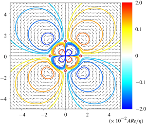
The presence of turbulent spots in planar shear flows is always accompanied by the existence of large-scale circulations. Reported examples include plane Poiseuille flow (Henningson & Kim Reference Henningson and Kim1991; Lemoult, Aider & Wesfreid Reference Lemoult, Aider and Wesfreid2013), plane Couette flow (Lundbladh & Johansson Reference Lundbladh and Johansson1991; Lagha & Manneville Reference Lagha and Manneville2007; Duguet & Schlatter Reference Duguet and Schlatter2013; Couliou & Monchaux Reference Couliou and Monchaux2015) and Waleffe flow (Schumacher & Eckhardt Reference Schumacher and Eckhardt2001; Chantry et al. Reference Chantry, Tuckerman and Barkley2016). Despite their different driving mechanisms, symmetries and boundary conditions, the large-scale flows in these planar systems share several properties. The wall-normal velocity features small-scale fluctuations which decay rapidly away from the spot (Eckhardt & Pandit Reference Eckhardt and Pandit2003). The large-scale in-plane velocities vary more slowly, they are directed inward along the streamwise direction and outward along the spanwise direction, giving rise to a quadrupolar circulation.
In the present study, we focus on the case of plane Couette flow. The associated linear base flow profile is known to be linearly stable for all Reynolds numbers (Romanov Reference Romanov1973), here defined as  $Re=Uh/\unicode[STIX]{x1D708}$, where
  $\pm U$ is the speed of counter-moving plates,
  $h$ is the half-gap size between them and
  $\unicode[STIX]{x1D708}$ is the kinematic viscosity of the fluid. It admits a simple analytical expression for the base flow:
  $\boldsymbol{U}=(Sy,0,0)$, where the shear
  $S=U/h$. The homogeneous shear of the base flow leads to plausible mathematical simplifications, while the absence of mean advection makes the long-term tracking of turbulent spots simpler. Therefore, plane Couette flow is an ideal system for analytical and experimental studies of localised turbulent spots and for the investigation of the large-scale flows around them.
Turbulent spots in plane Couette flow are sustained above  $Re\approx 325$ and take a rhombic shape, with the dimension along the streamwise direction being slightly larger than its counterpart in the spanwise direction (Daviaud et al. Reference Daviaud, Hegseth and Bergé1992; Tillmark & Alfredsson Reference Tillmark and Alfredsson1992; Dauchot & Daviaud Reference Dauchot and Daviaud1995a; Couliou & Monchaux Reference Couliou and Monchaux2018). During its initial growth, a turbulent spot undergoes a spanwise expansion resulting from two combined mechanisms: the stochastic nucleation of new streaks at the spanwise laminar–turbulent interface (Duguet et al. Reference Duguet, Maitre and Schlatter2011) and the motion of the interface due to the spanwise advection by large-scale flows (Duguet & Schlatter Reference Duguet and Schlatter2013; Couliou & Monchaux Reference Couliou and Monchaux2016, Reference Couliou and Monchaux2017). At later stages, growing turbulent spots start to distort and several spots might interact with each other. Two neighbouring spots can approach and merge, forming a single stripe inclined with respect to the streamwise direction (Duguet et al. Reference Duguet, Schlatter and Henningson2010). Moreover, large-scale flows introduce modifications to the base flow and depending on their far-field decay, they may contribute to a long-range modulation among turbulent spots (Prigent et al. Reference Prigent, Grégoire, Chaté, Dauchot and van Saarloos2002, Reference Prigent, Grégoire, Chaté and Dauchot2003), leading to the formation of laminar–turbulent banded patterns or labyrinths (Barkley & Tuckerman Reference Barkley and Tuckerman2007; Duguet et al. Reference Duguet, Schlatter and Henningson2010). Therefore, in order to understand the underlying mechanism for the spreading and suppression of localised turbulence by large-scale flows and to formulate an interaction rule among spots, it is necessary to know how the large-scale flow intensities decay with the distance from the spot.
For  $Re<325$ turbulent spots in plane Couette flow are not sustained. However, they can be sustained artificially if they are continuously forced by the presence of a permanent disturbance, e.g. a transverse jet (Daviaud et al. Reference Daviaud, Hegseth and Bergé1992; Tillmark & Alfredsson Reference Tillmark and Alfredsson1992) or a solid obstacle (Bottin, Dauchot & Daviaud Reference Bottin, Dauchot and Daviaud1997; Couliou & Monchaux Reference Couliou and Monchaux2017). Even at low Reynolds numbers
  $Re\leqslant 10$, a continuous forcing localised in space triggers a permanent response interpretable as a non-turbulent spot (Tardu Reference Tardu2012).
The physical origin of the large-scale flow is the mismatch of the streamwise flow rates across the laminar–turbulent interface (Duguet & Schlatter Reference Duguet and Schlatter2013). The mismatch is associated with the presence of overhang regions, where the flow is turbulent near one wall and laminar near the other (Coles Reference Coles1965; Lundbladh & Johansson Reference Lundbladh and Johansson1991). The scaling behaviour of the large-scale flows away from turbulent spots is far from clear and even controversial. Schumacher & Eckhardt (Reference Schumacher and Eckhardt2001) have investigated the growth of turbulent spots in Waleffe flow. By averaging between the two walls, they observed quadrupolar flows apparently similar to those in plane Couette flow with no-slip boundary conditions (Duguet & Schlatter Reference Duguet and Schlatter2013; Couliou & Monchaux Reference Couliou and Monchaux2016). In a moderate periodic domain of size  $80h\times 2h\times 80h$, where
  $2h$ is the gap width, they found that the kinetic energy of the large-scale flow exhibits an exponential decay in space, with a decay rate almost independent of the turbulent fluctuations inside the spot. More recently, Brand & Gibson (Reference Brand and Gibson2014) analysed a localised steady solution of plane Couette flow in a periodic domain of size
  $200h\times 2h\times 200h$. They found that the quadrupolar flow decays exponentially in both streamwise and spanwise directions, thereby supporting the previous observation by Schumacher & Eckhardt (Reference Schumacher and Eckhardt2001). However, closer examination of the database obtained in Duguet & Schlatter (Reference Duguet and Schlatter2013) reveals a deviation from the exponential scaling for turbulent spots in larger computation domains, though no scaling rule can be firmly established. In experiments by Couliou & Monchaux (Reference Couliou and Monchaux2015), no clear scaling has emerged from the data due to the difficulty of measuring low-amplitude velocities.
Despite the ubiquitous observation of spots in experiments and direct numerical simulations, as well as their importance for understanding growth dynamics and pattern formation, no analytical solution for quadrupolar flows has been obtained by solving the Navier–Stokes equations. In this work, we present an analytical derivation for quadrupolar circulations in a flow with a linear laminar profile, but confined by free-slip boundary conditions at the walls, instead of no slip. As we shall see, such a trade-off is a necessary compromise for the analytical approach. The reasons for choosing to accomplish an analytical study are (i) the current technical limitations in addressing experimentally or numerically the prediction of the far-field decay and (ii) the general lack of analytical studies on spatial localisation in the Navier–Stokes equations and their importance for a genuine understanding of the underlying localisation mechanisms.
The plan of the paper is as follows: a derivation of equations governing the large-scale flow is given in § 2, in addition to a modelling of turbulent spots based on symmetry arguments. In § 3, the proposed governing equations for the poloidal and toroidal functions are supplemented with free-slip boundary conditions and solved analytically. The characteristics of the quadrupolar flow are recovered in § 4 from the poloidal and toroidal functions, along with a brief argument for the topological origin of quadrupolar circulation in planar shear flows. Finally, conclusions drawn from the present study and outlooks are given in § 5.
2 Formulation
In this section, we present a derivation for a linearised model characterising the spatial distribution of the large-scale flow. Throughout the derivation, two assumptions have been exploited: (i) the intensity separation between the large-scale flow in the far field and the relative speed of counter-moving plates in § 2.1; and (ii) the scale separation between the wall-normal and the homogeneous directions in § 2.2. In order to solve the derived model, boundary conditions are discussed in § 2.4 and the forcing term representing a localised turbulent spot is modelled in § 2.5.
2.1 Linearised Navier–Stokes equations
Turbulent spots in plane Couette flow are limited to a bounded region in two homogeneous directions, but extend all the way across the gap. Localised distribution of the small-scale turbulent fluctuations inside the spot leads to the large-scale flow penetrating deeply into the laminar regions. At large distances from the spot, the decaying large-scale flow contributes to a weak deviation from the laminar base flow. Following Li & Widnall (Reference Li and Widnall1989), we consider a decomposition of the instantaneous flow characteristics, i.e. the velocity  $\boldsymbol{u}$ and the pressure
  $p$, into a base flow
  $(\boldsymbol{U},P)$, turbulent fluctuations
  $(\boldsymbol{u}^{\prime },p^{\prime })$ inside the turbulent spot and a perturbation
  $(\tilde{\boldsymbol{u}},\tilde{p})$ representing the large-scale flow
 $$\begin{eqnarray}\boldsymbol{u}=\boldsymbol{U}+\boldsymbol{u}^{\prime }+\tilde{\boldsymbol{u}},\quad p=P+p^{\prime }+\tilde{p},\end{eqnarray}$$
where, denoting by overbar the ensemble averaging, the large-scale flow is given by
 $$\begin{eqnarray}\tilde{\boldsymbol{u}}=\overline{\boldsymbol{u}-\boldsymbol{U}},\quad \tilde{p}=\overline{p-P}.\end{eqnarray}$$
 By taking the ensemble average of the Navier–Stokes equations, in Cartesian coordinates, where the axes  $x$,
$x$,  $y$ and
  $z$ are aligned with the streamwise, wall-normal and spanwise directions, the large-scale flow
  $(\tilde{\boldsymbol{u}},\tilde{p})$ is governed by
 $$\begin{eqnarray}\displaystyle & \displaystyle D_{t}\tilde{\boldsymbol{u}}+\tilde{\boldsymbol{u}}\boldsymbol{\cdot }\unicode[STIX]{x1D735}\boldsymbol{U}+\overline{\boldsymbol{u}^{\prime }\boldsymbol{\cdot }\unicode[STIX]{x1D735}\boldsymbol{u}^{\prime }}=-\unicode[STIX]{x1D70C}^{-1}\unicode[STIX]{x1D735}\tilde{p}+\unicode[STIX]{x1D708}\unicode[STIX]{x1D6FB}^{2}\tilde{\boldsymbol{u}}, & \displaystyle\end{eqnarray}$$
 $$\begin{eqnarray}\displaystyle & \displaystyle \unicode[STIX]{x1D735}\boldsymbol{\cdot }\tilde{\boldsymbol{u}}=0, & \displaystyle\end{eqnarray}$$
 where  $\unicode[STIX]{x1D70C}$ is the fluid density and
 $$\begin{eqnarray}D_{t}=\unicode[STIX]{x2202}_{t}+\boldsymbol{U}\boldsymbol{\cdot }\unicode[STIX]{x1D735}\end{eqnarray}$$
 denotes the material derivative. In (2.3), terms that are quadratic in  $\tilde{\boldsymbol{u}}$ are neglected, reflecting the observation that the large-scale flow is a weak perturbation on the background laminar shear flow, that is
  $|\tilde{\boldsymbol{u}}|\ll U$. The preceding equations are supplemented with the Dirichlet boundary conditions
 $$\begin{eqnarray}\boldsymbol{u}^{\prime }=\tilde{\boldsymbol{u}}=0,\end{eqnarray}$$
 at the walls  $y=\pm h$ and at infinity, i.e.
  $|x|,|z|\rightarrow \infty$.
Note that, subjected to the shearing of the base flow, perturbations generated at the spot are advected away and decay in amplitude. Since, our focus is on the large-scale flow in the far field, not flow structures inside turbulent spots, we propose to seek invariant solutions  $\tilde{\boldsymbol{u}}(x_{L},y_{L},z_{L})$ in a co-moving Lagrangian frame attached to the base flow
 $$\begin{eqnarray}x_{L}=x-Syt,\quad y_{L}=y,\quad z_{L}=z,\end{eqnarray}$$
 where the subscript  $_{L}$ denotes variables in the Lagrangian frame. Hence
 $$\begin{eqnarray}D_{t}\tilde{\boldsymbol{u}}=0.\end{eqnarray}$$
This assumption coincides with Kelvin’s solution for ship wakes (Kelvin Reference Kelvin1887) and Taylor’s hypothesis on turbulence (Taylor Reference Taylor1938). The fulfilment of the Lagrangian invariance with our solution for quadrupolar flows is inspected in § 3.1 and § 4.1, respectively.
By applying the divergence operator to (2.3) and using equation (2.4), the Poisson equation for pressure is
 $$\begin{eqnarray}\unicode[STIX]{x1D70C}^{-1}\unicode[STIX]{x1D6FB}^{2}\tilde{p}=-2S\unicode[STIX]{x2202}_{x}\tilde{u} _{y}-\unicode[STIX]{x1D735}\boldsymbol{\cdot }\overline{\boldsymbol{u}^{\prime }\boldsymbol{\cdot }\unicode[STIX]{x1D735}\boldsymbol{u}^{\prime }}.\end{eqnarray}$$
It is seen that the perturbed pressure comes from two distinct origins: (i) the spatial variation of the perturbed velocity, and (ii) the divergence of the Reynolds stresses. Consequently, the perturbed pressure can be further decomposed into
 $$\begin{eqnarray}\tilde{p}=\tilde{p}^{(i)}+\tilde{p}^{(ii)},\end{eqnarray}$$
 where  $\tilde{p}^{(ii)}$ is denoted, up to an additive constant, by
 $$\begin{eqnarray}\unicode[STIX]{x1D70C}^{-1}\unicode[STIX]{x1D6FB}^{2}\tilde{p}^{(ii)}=-\unicode[STIX]{x1D735}\boldsymbol{\cdot }\overline{\boldsymbol{u}^{\prime }\boldsymbol{\cdot }\unicode[STIX]{x1D735}\boldsymbol{u}^{\prime }}.\end{eqnarray}$$
 It is seen from (2.11) that, since the Reynolds stresses are not divergence free, the divergence of the Reynolds stresses will always generate a corresponding pressure field  $\tilde{p}^{(ii)}$ so as to make the sum
 $$\begin{eqnarray}\boldsymbol{q}_{\tilde{\boldsymbol{u}}}=-\overline{\boldsymbol{u}^{\prime }\boldsymbol{\cdot }\unicode[STIX]{x1D735}\boldsymbol{u}^{\prime }}-\unicode[STIX]{x1D70C}^{-1}\unicode[STIX]{x1D735}\tilde{p}^{(ii)},\end{eqnarray}$$
satisfy the incompressible condition
 $$\begin{eqnarray}\unicode[STIX]{x1D735}\boldsymbol{\cdot }\boldsymbol{q}_{\tilde{\boldsymbol{u}}}=0.\end{eqnarray}$$
 This observation reflects the mathematical fact that, for incompressible flows, the role of the pressure is to project the compressible nonlinear terms onto the subspace of divergence-free flow fields. Therefore, we interpret  $\boldsymbol{q}_{\tilde{\boldsymbol{u}}}$ as a forcing term mimicking the presence of an autonomous turbulent spot.
By using equations (2.8) and (2.12), and dropping the superscript  $^{(i)}$ denoting the origin, the momentum equation (2.3) can be expressed as
 $$\begin{eqnarray}\tilde{\boldsymbol{u}}\boldsymbol{\cdot }\unicode[STIX]{x1D735}\boldsymbol{U}=-\unicode[STIX]{x1D70C}^{-1}\unicode[STIX]{x1D735}\tilde{p}+\unicode[STIX]{x1D708}\unicode[STIX]{x1D6FB}^{2}\tilde{\boldsymbol{u}}+\boldsymbol{q}_{\tilde{\boldsymbol{ u}}},\end{eqnarray}$$
where the incompressibility constraint (2.4) leads to the following Poisson equation
 $$\begin{eqnarray}\unicode[STIX]{x1D70C}^{-1}\unicode[STIX]{x1D6FB}^{2}\tilde{p}=-2S\unicode[STIX]{x2202}_{x}\tilde{u} _{y}.\end{eqnarray}$$
Due to the presence of the variable part of the pressure gradient in (2.12), the forcing term need not vanish at the walls. However, in order to simplify the algebra, we impose the Dirichlet boundary conditions for the forcing
 $$\begin{eqnarray}\boldsymbol{q}_{\tilde{\boldsymbol{u}}}|_{y=\pm h}=0,\end{eqnarray}$$
complementary to the boundary conditions (2.6). Another calculation without imposing the Dirichlet boundary condition (2.16) yields similar results (Wang Reference Wang2019). Alternatively, Li & Widnall (Reference Li and Widnall1989) and Lagha & Manneville (Reference Lagha and Manneville2007) have modelled an isolated turbulent spot as a Gaussian distribution of Reynolds stresses in the homogeneous directions, deviating from the current approach.
2.2 Geometric scale separation in plane Couette flow
A distinguishing feature of planar shear flows is that, unlike localised turbulent fluctuations, the large-scale flow is spatially extended in the homogeneous directions, whereas highly confined in the wall-normal direction due to the presence of walls. Since the large-scale flows do not present an obvious well-defined length scale, let us denote by  $\unicode[STIX]{x1D706}$ the distance from a localised turbulent spot to where the large-scale flow is measured. The planar geometry entails the existence of a small parameter
 $$\begin{eqnarray}\unicode[STIX]{x1D702}=h/\unicode[STIX]{x1D706}\ll 1.\end{eqnarray}$$
 This slenderness is associated with a separation of geometric scales. Due to the confinement by the walls, the perturbed flow occurs at length scales  ${\approx}h$ in the wall-normal direction, while it is extended in the homogeneous directions. In a periodic box of size
  $[500h,2h,500h]$, for instance, the large-scale flow is observed at scales
  $\unicode[STIX]{x1D706}\approx 100h$, cf. figure 3 in Duguet & Schlatter (Reference Duguet and Schlatter2013). For this particular case,
  $\unicode[STIX]{x1D702}\approx 10^{-2}$ measures the separation between the small and large scales.
In this study, we suggest to exploit this geometric scale separation. We thus rescale the homogeneous coordinates  $x$ and
  $z$ by
  $\unicode[STIX]{x1D706}$, and the wall-normal coordinate
  $y$ by
  $h$
$h$
 $$\begin{eqnarray}x=\unicode[STIX]{x1D706}x^{\ast },\quad y=hy^{\ast },\quad z=\unicode[STIX]{x1D706}z^{\ast },\end{eqnarray}$$
 where the superscript  $^{\ast }$ denotes rescaled dimensionless variables. As such, the walls are now located at
  $y=\pm 1$. We choose to rescale in-plane velocities by
  $U$. The incompressibility constraints (2.4) and (2.13) lead to the following substitution for the velocity components
 $$\begin{eqnarray}\tilde{u} _{x}=U\tilde{u} _{x}^{\ast },\quad \tilde{u} _{y}=\unicode[STIX]{x1D702}U\tilde{u} _{y}^{\ast },\quad \tilde{u} _{z}=U\tilde{u} _{z}^{\ast },\end{eqnarray}$$
and for the forcing
 $$\begin{eqnarray}q_{\tilde{u} _{x}}=(\unicode[STIX]{x1D708}U/h^{2})q_{\tilde{u} _{x}}^{\ast },\quad q_{\tilde{u} _{y}}=\unicode[STIX]{x1D702}(\unicode[STIX]{x1D708}U/h^{2})q_{\tilde{u} _{y}}^{\ast },\quad q_{\tilde{u} _{z}}=(\unicode[STIX]{x1D708}U/h^{2})q_{\tilde{u} _{z}}^{\ast },\end{eqnarray}$$
where the scaling for the forcing terms is selected so as to balance the viscous dissipation. Similarly, the scaling for the pressure, as in lubrication theory (Howison Reference Howison2005)
 $$\begin{eqnarray}\tilde{p}=\unicode[STIX]{x1D70C}(\unicode[STIX]{x1D708}U\unicode[STIX]{x1D706}/h^{2})\tilde{p}^{\ast },\end{eqnarray}$$
 is built on a balance between the pressure gradients and the dominant viscous terms in the homogeneous directions. Note that the scaling (2.21) is justified provided that the reduced Reynolds number  $\unicode[STIX]{x1D6FC}$ is small
 $$\begin{eqnarray}\unicode[STIX]{x1D6FC}=\unicode[STIX]{x1D702}Re\ll 1.\end{eqnarray}$$
 This condition is satisfied as soon as the scale separation  $\unicode[STIX]{x1D702}^{-1}$ sufficiently large, cf. equation (2.17), and it shall be assumed henceforth.
Substituting the preceding scaling relations into (2.14), the rescaled non-dimensional Navier–Stokes equations are
 $$\begin{eqnarray}\displaystyle & \displaystyle (\unicode[STIX]{x1D702}^{2}\unicode[STIX]{x2202}_{x^{\ast }}^{2}+\unicode[STIX]{x2202}_{y^{\ast }}^{2}+\unicode[STIX]{x1D702}^{2}\unicode[STIX]{x2202}_{z^{\ast }}^{2})\tilde{u} _{x}^{\ast }=\unicode[STIX]{x2202}_{x^{\ast }}\tilde{p}^{\ast }+\unicode[STIX]{x1D6FC}\tilde{u} _{y}^{\ast }-q_{\tilde{u} _{x}}^{\ast }, & \displaystyle\end{eqnarray}$$
 $$\begin{eqnarray}\displaystyle & \displaystyle (\unicode[STIX]{x1D702}^{2}\unicode[STIX]{x2202}_{x^{\ast }}^{2}+\unicode[STIX]{x2202}_{y^{\ast }}^{2}+\unicode[STIX]{x1D702}^{2}\unicode[STIX]{x2202}_{z^{\ast }}^{2})\tilde{u} _{y}^{\ast }=\unicode[STIX]{x1D702}^{-2}\unicode[STIX]{x2202}_{y^{\ast }}\tilde{p}^{\ast }-q_{\tilde{u} _{y}}^{\ast }, & \displaystyle\end{eqnarray}$$
 $$\begin{eqnarray}\displaystyle & \displaystyle (\unicode[STIX]{x1D702}^{2}\unicode[STIX]{x2202}_{x^{\ast }}^{2}+\unicode[STIX]{x2202}_{y^{\ast }}^{2}+\unicode[STIX]{x1D702}^{2}\unicode[STIX]{x2202}_{z^{\ast }}^{2})\tilde{u} _{z}^{\ast }=\unicode[STIX]{x2202}_{z^{\ast }}\tilde{p}^{\ast }-q_{\tilde{u} _{z}}^{\ast }, & \displaystyle\end{eqnarray}$$
 $$\begin{eqnarray}(\unicode[STIX]{x2202}_{x^{\ast }}^{2}+\unicode[STIX]{x1D702}^{-2}\unicode[STIX]{x2202}_{y^{\ast }}^{2}+\unicode[STIX]{x2202}_{z^{\ast }}^{2})\tilde{p}^{\ast }=-2\unicode[STIX]{x1D6FC}\unicode[STIX]{x2202}_{x^{\ast }}\tilde{u} _{y}^{\ast }.\end{eqnarray}$$
 In contrast to lubrication theory, wherein the Laplace operator reduces to a second-order derivative with respect to  $y^{\ast }$, the full operator is retained here.
We observe from (2.23b) that the vertical pressure gradient is larger, by a factor  $\unicode[STIX]{x1D702}^{-2}$, than remaining terms in the equation, hence it cannot be balanced. The formal procedure consists of expanding the perturbed pressure as
 $$\begin{eqnarray}\tilde{p}^{\ast }=\tilde{p}^{\ast (0)}+\unicode[STIX]{x1D702}^{2}\tilde{p}^{\ast (1)}+O(\unicode[STIX]{x1D702}^{4}).\end{eqnarray}$$
 Substituting the expansion into equations (2.23) and collecting powers of  $\unicode[STIX]{x1D702}^{-2}$ reveals that
 $$\begin{eqnarray}\unicode[STIX]{x2202}_{y^{\ast }}\tilde{p}^{\ast (0)}=0.\end{eqnarray}$$
 This means that, due to the confinement by the walls, the leading-order pressure  $\tilde{p}^{\ast (0)}$ is only effective in generating large-scale flows in the homogeneous directions. The first-order correction
  $\tilde{p}^{\ast (1)}$ enters equation (2.23b), generating small-scale vertical motions of
  $O(h)$, but has negligible effect on generating the large-scale in-plane flows of
  $O(\unicode[STIX]{x1D706})$. Since equations (2.23) are linear and since we are interested in the angular dependence and scaling characteristics of the large-scale flows, we filter out the irrelevant small-scale vertical motions by truncating the perturbative expansion (2.25) to the lowest order
 $$\begin{eqnarray}\tilde{p}^{\ast }=\tilde{p}^{\ast (0)}.\end{eqnarray}$$
Substituting the truncation (2.27) into equations (2.23) and using (2.26), we obtain
 $$\begin{eqnarray}\displaystyle & \displaystyle (\unicode[STIX]{x1D702}^{2}\unicode[STIX]{x2202}_{x^{\ast }}^{2}+\unicode[STIX]{x2202}_{y^{\ast }}^{2}+\unicode[STIX]{x1D702}^{2}\unicode[STIX]{x2202}_{z^{\ast }}^{2})\tilde{u} _{x}^{\ast }=\unicode[STIX]{x2202}_{x^{\ast }}\tilde{p}^{\ast }+\unicode[STIX]{x1D6FC}\tilde{u} _{y}^{\ast }-q_{\tilde{u} _{x}}^{\ast }, & \displaystyle\end{eqnarray}$$
 $$\begin{eqnarray}\displaystyle & \displaystyle (\unicode[STIX]{x1D702}^{2}\unicode[STIX]{x2202}_{x^{\ast }}^{2}+\unicode[STIX]{x2202}_{y^{\ast }}^{2}+\unicode[STIX]{x1D702}^{2}\unicode[STIX]{x2202}_{z^{\ast }}^{2})\tilde{u} _{y}^{\ast }=-q_{\tilde{u} _{y}}^{\ast }, & \displaystyle\end{eqnarray}$$
 $$\begin{eqnarray}\displaystyle & \displaystyle (\unicode[STIX]{x1D702}^{2}\unicode[STIX]{x2202}_{x^{\ast }}^{2}+\unicode[STIX]{x2202}_{y^{\ast }}^{2}+\unicode[STIX]{x1D702}^{2}\unicode[STIX]{x2202}_{z^{\ast }}^{2})\tilde{u} _{z}^{\ast }=\unicode[STIX]{x2202}_{z^{\ast }}\tilde{p}^{\ast }-q_{\tilde{u} _{z}}^{\ast }. & \displaystyle\end{eqnarray}$$
For completeness, the perturbed pressure can be recovered by solving the following two-dimensional Poisson equation
 $$\begin{eqnarray}(\unicode[STIX]{x2202}_{x^{\ast }}^{2}+\unicode[STIX]{x2202}_{z^{\ast }}^{2})\tilde{p}^{\ast }=-2\unicode[STIX]{x1D6FC}\unicode[STIX]{x2202}_{x^{\ast }}\tilde{u} _{y}^{\ast },\end{eqnarray}$$
as soon as the wall-normal velocity is determined.
2.3 Poloidal–toroidal decomposition
In order to guarantee that the validity of the incompressible constraints (2.4) and (2.13) is not effected by the truncation (2.27), we represent the perturbed velocity  $\tilde{\boldsymbol{u}}$ using the poloidal–toroidal decomposition
 $$\begin{eqnarray}\tilde{\boldsymbol{u}}^{\ast }=\unicode[STIX]{x1D735}^{\ast }\times (\tilde{\unicode[STIX]{x1D713}}^{\ast }\boldsymbol{e}_{y})+\unicode[STIX]{x1D735}^{\ast }\times \unicode[STIX]{x1D735}^{\ast }\times (\tilde{\unicode[STIX]{x1D719}}^{\ast }\boldsymbol{e}_{y}),\end{eqnarray}$$
 where  $\unicode[STIX]{x1D735}^{\ast }=(\unicode[STIX]{x1D702}\unicode[STIX]{x2202}_{x^{\ast }},\unicode[STIX]{x2202}_{y^{\ast }},\unicode[STIX]{x1D702}\unicode[STIX]{x2202}_{z^{\ast }})$ is now the scaled gradient operator,
  $\tilde{\unicode[STIX]{x1D719}}^{\ast }$ and
  $\tilde{\unicode[STIX]{x1D713}}^{\ast }$ are the poloidal and toroidal functions, respectively, and
  $\boldsymbol{e}_{y}$ is the unit vector pointing towards positive
  $y$. Similarly, the forcing term
  $\boldsymbol{q}_{\tilde{\boldsymbol{u}}}^{\ast }$ can be expressed in terms of the poloidal
  $q_{\tilde{\unicode[STIX]{x1D719}}}^{\ast }$ and the toroidal
  $q_{\tilde{\unicode[STIX]{x1D713}}}^{\ast }$ components as
 $$\begin{eqnarray}\boldsymbol{q}_{\tilde{\boldsymbol{u}}}^{\ast }=\unicode[STIX]{x1D735}^{\ast }\times (q_{\tilde{\unicode[STIX]{x1D713}}}^{\ast }\boldsymbol{e}_{y})+\unicode[STIX]{x1D735}^{\ast }\times \unicode[STIX]{x1D735}^{\ast }\times (q_{\tilde{\unicode[STIX]{x1D719}}}^{\ast }\boldsymbol{e}_{y}).\end{eqnarray}$$
Hence, rather than working with the three-dimensional velocity field, we pursue in this paper the poloidal–toroidal formulation à la Marqués (Reference Marqués1990)
 $$\begin{eqnarray}\displaystyle & \displaystyle (\unicode[STIX]{x1D702}^{2}\unicode[STIX]{x2202}_{x}^{2}+\unicode[STIX]{x2202}_{y}^{2}+\unicode[STIX]{x1D702}^{2}\unicode[STIX]{x2202}_{z}^{2})\tilde{\unicode[STIX]{x1D719}}=-q_{\tilde{\unicode[STIX]{x1D719}}}, & \displaystyle\end{eqnarray}$$
 $$\begin{eqnarray}\displaystyle & \displaystyle (\unicode[STIX]{x1D702}^{2}\unicode[STIX]{x2202}_{x}^{2}+\unicode[STIX]{x2202}_{y}^{2}+\unicode[STIX]{x1D702}^{2}\unicode[STIX]{x2202}_{z}^{2})\tilde{\unicode[STIX]{x1D713}}=-q_{\tilde{\unicode[STIX]{x1D713}}}+\unicode[STIX]{x1D702}\unicode[STIX]{x1D6FC}\unicode[STIX]{x2202}_{z}\tilde{\unicode[STIX]{x1D719}}, & \displaystyle\end{eqnarray}$$
 $^{\ast }$ denoting rescaled dimensionless variables is now dropped for simplicity. Here, equation (2.32a) is obtained by substituting the decomposition (2.30) and (2.31) into equation (2.28b), while equation (2.32b) is obtained by taking the curl of (2.28) and projecting onto the
  $\boldsymbol{e}_{y}$ component. In order to simplify the expression, the two-dimensional Laplace operator
  $(\unicode[STIX]{x2202}_{x}^{2}+\unicode[STIX]{x2202}_{z}^{2})$ has been removed from both sides of (2.32). Consequently,
  $\tilde{\unicode[STIX]{x1D719}}$ and
  $\tilde{\unicode[STIX]{x1D713}}$ are determined only up to an additive function
  $h_{\tilde{\unicode[STIX]{x1D719}}}(x,z)$ and
  $h_{\tilde{\unicode[STIX]{x1D713}}}(x,z)$ satisfying the two-dimensional Laplace equations
  $$\begin{eqnarray}(\unicode[STIX]{x2202}_{x}^{2}+\unicode[STIX]{x2202}_{z}^{2})h_{\tilde{\unicode[STIX]{x1D719}}}(x,z)=(\unicode[STIX]{x2202}_{x}^{2}+\unicode[STIX]{x2202}_{z}^{2})h_{\tilde{\unicode[STIX]{x1D713}}}(x,z)=0.\end{eqnarray}$$
Stemming from the Dirichlet boundary conditions (2.6), equation (2.33) is supplemented with boundary conditions
 $$\begin{eqnarray}h_{\tilde{\unicode[STIX]{x1D719}}}(x,z)|_{|x|,|z|\rightarrow \infty }=h_{\tilde{\unicode[STIX]{x1D713}}}(x,z)|_{|x|,|z|\rightarrow \infty }=0,\end{eqnarray}$$
 such that  $h_{\tilde{\unicode[STIX]{x1D719}}}(x,z)$ and
  $h_{\tilde{\unicode[STIX]{x1D713}}}(x,z)$ are identically zero
 $$\begin{eqnarray}h_{\tilde{\unicode[STIX]{x1D719}}}(x,z)=h_{\tilde{\unicode[STIX]{x1D713}}}(x,z)=0.\end{eqnarray}$$
 Therefore,  $\tilde{\unicode[STIX]{x1D719}}$ and
  $\tilde{\unicode[STIX]{x1D713}}$ are uniquely determined by the second-order differential equations (2.32). Similarly, combining equations (2.29) and (2.30) and taking out the two-dimensional Laplace operator
  $(\unicode[STIX]{x2202}_{x}^{2}+\unicode[STIX]{x2202}_{z}^{2})$, the perturbed pressure becomes
 $$\begin{eqnarray}\tilde{p}=2\unicode[STIX]{x1D702}^{2}\unicode[STIX]{x1D6FC}\unicode[STIX]{x2202}_{x}\tilde{\unicode[STIX]{x1D719}}.\end{eqnarray}$$
 The preceding equations can be solved classically using Fourier transforms as soon as the boundary conditions as well as the forcing terms  $q_{\tilde{\unicode[STIX]{x1D719}}}$ and
  $q_{\tilde{\unicode[STIX]{x1D713}}}$ are specified.
2.4 Boundary conditions
The original boundary conditions for the plane Couette problem are no slip (2.6), which can be expressed in terms of the wall-normal components of the velocity and vorticity as
 $$\begin{eqnarray}\tilde{u} _{y}|_{y=\pm 1}=\unicode[STIX]{x2202}_{y}\tilde{u} _{y}|_{y=\pm 1}=\tilde{\unicode[STIX]{x1D714}}_{y}|_{y=\pm 1}=0.\end{eqnarray}$$
Stemming from the poloidal–toroidal decomposition (2.30), there is a correspondence between the velocity–vorticity and poloidal–toroidal formulations
 $$\begin{eqnarray}\displaystyle & \displaystyle \tilde{u} _{y}=-\unicode[STIX]{x1D702}^{2}(\unicode[STIX]{x2202}_{x}^{2}+\unicode[STIX]{x2202}_{z}^{2})\tilde{\unicode[STIX]{x1D719}}, & \displaystyle\end{eqnarray}$$
 $$\begin{eqnarray}\displaystyle & \displaystyle \tilde{\unicode[STIX]{x1D714}}_{y}=-\unicode[STIX]{x1D702}^{2}(\unicode[STIX]{x2202}_{x}^{2}+\unicode[STIX]{x2202}_{z}^{2})\tilde{\unicode[STIX]{x1D713}}. & \displaystyle\end{eqnarray}$$
Hence, the preceding no-slip boundary condition (2.37) can be rewritten in terms of the poloidal and toroidal functions as
 $$\begin{eqnarray}\tilde{\unicode[STIX]{x1D719}}|_{y=\pm 1}=\unicode[STIX]{x2202}_{y}\tilde{\unicode[STIX]{x1D719}}|_{y=\pm 1}=\tilde{\unicode[STIX]{x1D713}}|_{y=\pm 1}=0.\end{eqnarray}$$
 Here, the constraints on  $\unicode[STIX]{x2202}_{y}\tilde{\unicode[STIX]{x1D719}}$ and
  $\tilde{\unicode[STIX]{x1D713}}$ together ensure that the tangential velocities vanish at the walls. Note that there are four boundary conditions imposed on
  $\tilde{\unicode[STIX]{x1D719}}$, compatible with the presence of the fourth-order differential operator
  $\unicode[STIX]{x1D6FB}^{4}$ in the original momentum equation for
  $\tilde{\unicode[STIX]{x1D719}}$, cf. equation (14b) in Marqués (Reference Marqués1990). In this work, however, the removal of the vertical pressure gradient, which arises as a natural consequence of the geometric scale separation (2.17), not only filters out irrelevant small-scale motions driven by the vertical pressure gradient, but also leads to mathematical simplifications by reducing the fourth-order differential equation with respect to
  $y$ to a second-order one. Therefore, equation (2.32a) can support only two boundary conditions at the walls. This observation implies that the filtered small-scale motions must play a dominant role in satisfying the no-slip boundary conditions (2.40). Consequently, by removing them, we have to relax the no-slip boundary conditions to free-slip boundary conditions in order to ensure that the resulting problem is mathematically well posed.
Numerical simulations of Waleffe flow with stress-free boundary conditions (as considered by Schumacher & Eckhardt (Reference Schumacher and Eckhardt2001), Chantry et al. (Reference Chantry, Tuckerman and Barkley2016) and Chantry, Tuckerman & Barkley (Reference Chantry, Tuckerman and Barkley2017)),
 $$\begin{eqnarray}\tilde{u} _{y}|_{y=\pm 1}=\unicode[STIX]{x2202}_{y}^{2}\tilde{u} _{y}|_{y=\pm 1}=\unicode[STIX]{x2202}_{y}\tilde{\unicode[STIX]{x1D714}}_{y}|_{y=\pm 1}=0,\end{eqnarray}$$
 suggest that the presence of slip at the walls does not affect the generic properties of the large-scale flow. The stress-free boundary conditions can be expressed in terms of  $\tilde{\unicode[STIX]{x1D719}}$ and
  $\tilde{\unicode[STIX]{x1D713}}$ as
 $$\begin{eqnarray}\tilde{\unicode[STIX]{x1D719}}|_{y=\pm 1}=\unicode[STIX]{x2202}_{y}^{2}\tilde{\unicode[STIX]{x1D719}}|_{y=\pm 1}=\unicode[STIX]{x2202}_{y}\tilde{\unicode[STIX]{x1D713}}|_{y=\pm 1}=0,\end{eqnarray}$$
 where vanishing  $\unicode[STIX]{x2202}_{y}^{2}\tilde{\unicode[STIX]{x1D719}}|_{y=\pm 1}$ and
  $\unicode[STIX]{x2202}_{y}\tilde{\unicode[STIX]{x1D713}}|_{y=\pm 1}$ ensure that the tangential stresses are zero at the walls. However, since the linear laminar profile of plane Couette flow does not satisfy the stress-free boundary conditions, one needs to modify the base flow by, for instance, the inclusion of a sinusoidal body force. Moreover, similar to the no-slip boundary conditions, there are four constraints imposed on
  $\tilde{\unicode[STIX]{x1D719}}$, incompatible with the second-order differential equation (2.32a). Therefore, in general, the stress-free boundary conditions (2.42) cannot be satisfied, unless
  $\tilde{\unicode[STIX]{x1D719}}$ solves
 $$\begin{eqnarray}\unicode[STIX]{x2202}_{y}^{2}\tilde{\unicode[STIX]{x1D719}}=c\tilde{\unicode[STIX]{x1D719}},\end{eqnarray}$$
 up to a multiplying constant  $c$. In this case, two constraints for
  $\tilde{\unicode[STIX]{x1D719}}$ are simultaneously satisfied. Examples include trigonometric and hyperbolic trigonometric functions.
As a compromise between the number of boundary conditions that can be imposed on equation (2.32a) and the compatibility with the linear base flow, we consider in this paper a flow with mixed boundary conditions as in Eckhardt & Pandit (Reference Eckhardt and Pandit2003). More specifically, we require that the laminar profile satisfies the no-slip boundary conditions (2.6) of the full Navier–Stokes equations, whereas the perturbation satisfies the following free-slip boundary conditions:
 $$\begin{eqnarray}\tilde{\unicode[STIX]{x1D719}}|_{y=\pm 1}=0\quad \text{and}\quad \unicode[STIX]{x2202}_{y}\tilde{\unicode[STIX]{x1D713}}|_{y=\pm 1}=0.\end{eqnarray}$$
 Here, the constraint on  $\tilde{\unicode[STIX]{x1D719}}$ signifies that there is no penetration at the walls, while the constraint on
  $\tilde{\unicode[STIX]{x1D713}}$ is borrowed from the stress-free boundary conditions (2.42). It is demonstrated in § 3.1 that the perturbed flow field obtained in this paper also satisfies the stress-free boundary conditions (2.42), while the generality of the proposed free-slip boundary conditions (2.44) is discussed from a topological point of view in § 4.4.
2.5 Forcing selection
By seeking an equilibrium solution in an Eulerian frame attached to spots, Li & Widnall (Reference Li and Widnall1989) obtained doubly localised solutions in plane Poiseuille flow. With the same assumption, Brand & Gibson (Reference Brand and Gibson2014) obtained a similar solution for plane Couette flow. Note that these solutions are similar in size and structure to turbulent spots obtained from direct numerical simulations. Consequently, rather than the detailed dynamics, we perceive large-scale flows as arising from the blockage effect of localised turbulent spots. This leads to a formulation of the forcing terms by making the minimal assumption in § 2.5.1. Based on the parity analysis of (2.32), we conclude in § 2.5.2 that the formation of quadrupolar flows is associated with the forcing components that are symmetric with respect of the mid-plane  $y=0$.
2.5.1 Minimal assumption model for a localised spot
In order to solve equations (2.32), we must specify an analytical form for the forcing  $(q_{\tilde{\unicode[STIX]{x1D719}}},q_{\tilde{\unicode[STIX]{x1D713}}})$, yet the selection must not predetermine the large-scale flow. As such, we make the minimal assumption by modelling a localised turbulent spot as an obstacle in the
  $xy$-plane, that will deflect the streamwise velocity into vertical momentum, without imposing a wall-normal vorticity distribution in the
  $xz$-plane. By virtue of the conservation of angular momentum, the vertical momentum will alternate sign on each side of the obstacle. Assuming that the vertical momentum is concentrated on a mathematical filament along the
  $y$-axis which terminates at the walls, the minimal forcing is
 $$\begin{eqnarray}\displaystyle & \displaystyle q_{\tilde{\unicode[STIX]{x1D719}}}=-Ag(y)\unicode[STIX]{x1D6FF}^{\prime }(x)\unicode[STIX]{x1D6FF}(z), & \displaystyle\end{eqnarray}$$
 $$\begin{eqnarray}\displaystyle & \displaystyle q_{\tilde{\unicode[STIX]{x1D713}}}=0. & \displaystyle\end{eqnarray}$$
 Here,  $A$ is the amplitude of the forcing and the prime, which denotes a derivative with respect to the scaled
  $x$-axis, i.e.
  $\unicode[STIX]{x1D702}\unicode[STIX]{x2202}_{x}$, arises as a consequence of opposite vertical momentum. Note that the poloidal forcing (2.45) imposes a counter-rotating pair of streamwise circulations in the
  $yz$-plane. The form factor
 $$\begin{eqnarray}g(y)|_{y=\pm 1}=0\end{eqnarray}$$
is adjusted so as to satisfy the Dirichlet boundary condition (2.16).
The sign of  $A$ remains undetermined, and it shall be concluded by comparing the analytic solution with previous experimental and numerical results in § 4.2. Denoting the integral
 $$\begin{eqnarray}G=\int _{-1}^{1}g(y)\,\text{d}y.\end{eqnarray}$$
 For  $AG>0$, the forcing term (2.45) introduces an overall spanwise vorticity which is opposite in sign to that of the base flow; whereas for
  $AG<0$, the spanwise vorticity associated with the spot is aligned with that of the base flow.
2.5.2 Parity of the forcing
Although the characteristics of turbulent spots, as well as of the large-scale flows around them, are strongly three-dimensional, the quadrupolar circulation is revealed at the mid-plane  $y=0$ or after applying the
  $y$-average, denoted by
 $$\begin{eqnarray}\langle \;\rangle =\frac{1}{2}\int _{-1}^{1}\,\text{d}y,\end{eqnarray}$$
 to the perturbed in-plane flow  $\langle \tilde{\boldsymbol{u}}_{2D}\rangle =(\langle \tilde{u} _{x}\rangle ,\langle \tilde{u} _{z}\rangle )$. Here, the
  $y$-averaged in-plane velocities
 $$\begin{eqnarray}\displaystyle & \displaystyle \langle \tilde{u} _{x}\rangle =-\unicode[STIX]{x1D702}\unicode[STIX]{x2202}_{z}\langle \tilde{\unicode[STIX]{x1D713}}\rangle +\unicode[STIX]{x1D702}\unicode[STIX]{x2202}_{x}\langle \unicode[STIX]{x2202}_{y}\tilde{\unicode[STIX]{x1D719}}\rangle , & \displaystyle\end{eqnarray}$$
 $$\begin{eqnarray}\displaystyle & \displaystyle \langle \tilde{u} _{z}\rangle =+\unicode[STIX]{x1D702}\unicode[STIX]{x2202}_{x}\langle \tilde{\unicode[STIX]{x1D713}}\rangle +\unicode[STIX]{x1D702}\unicode[STIX]{x2202}_{z}\langle \unicode[STIX]{x2202}_{y}\tilde{\unicode[STIX]{x1D719}}\rangle & \displaystyle\end{eqnarray}$$
 can be decomposed into a divergence-free component characterised by the streamfunction  $\langle \tilde{\unicode[STIX]{x1D713}}\rangle$ and a curl-free component characterised by the velocity potential
  $\langle \unicode[STIX]{x2202}_{y}\tilde{\unicode[STIX]{x1D719}}\rangle$. The latter is identically zero with the Dirichlet boundary conditions (2.44):
 $$\begin{eqnarray}\langle \unicode[STIX]{x2202}_{y}\tilde{\unicode[STIX]{x1D719}}\rangle ={\textstyle \frac{1}{2}}(\tilde{\unicode[STIX]{x1D719}}|_{y=+1}-\tilde{\unicode[STIX]{x1D719}}|_{y=-1})=0.\end{eqnarray}$$
 Therefore, the in-plane flow  $\langle \tilde{\boldsymbol{u}}_{2D}\rangle$ is divergence free, arising from the non-vanishing
  $\langle \tilde{\unicode[STIX]{x1D713}}\rangle$.
Since the differential operator in (2.32) is strictly second order, the parity of the poloidal and toroidal functions is uniquely determined by the parity of the forcing. More specifically, the odd component of  $q_{\tilde{\unicode[STIX]{x1D719}}}$ leads to
  $\tilde{\unicode[STIX]{x1D713}}$ vanishing upon
  $y$-averaging. Since
  $q_{\tilde{\unicode[STIX]{x1D713}}}$ is zero by assumption, the quadrupolar flow must stem from the even part of the forcing. Accordingly, we restrict ourselves to the case where
  $g(y)$ is an even function of
  $y$.
$y$.
Let  $g(y)$ be an arbitrary even function satisfying the Dirichlet boundary condition (2.47), it can be expanded using Fourier series as
 $$\begin{eqnarray}g(y)=\mathop{\sum }_{n=1}^{\infty }a_{n}\cos (\unicode[STIX]{x1D709}_{n}y),\end{eqnarray}$$
 where  $a_{n}$ denote the Fourier coefficients and the wavenumbers are discretised
 $$\begin{eqnarray}\unicode[STIX]{x1D709}_{n}=(n-{\textstyle \frac{1}{2}})\unicode[STIX]{x03C0}\quad \text{for }n=1,2,3\ldots\end{eqnarray}$$
 In this model, the index  $n$ signifies that there are
  $n$ mutually counter-rotating vortices stacking along the
  $y$-axis. Based on the minimal assumption meant to model a localised filament-like spot, the present analysis can be applied to not only the transitional flows with
  $Re\approx 300$ but to all regimes with
  $Re>0$ down to the Stokes regime.
3 Analytical solutions for poloidal and toroidal functions
In this section, the modal solutions for the poloidal and toroidal functions are presented in § 3.1 and their inverse Fourier transform are evaluated in § 3.2. Moreover, the origin of the quadrupolar angular dependence and the algebraic decay in the toroidal function is uncovered in §§ 3.1 and 3.2, respectively.
3.1 Modal solutions
The homogeneity in  $x$ and
  $z$ justifies the use of a Fourier transform in the corresponding directions with wavenumbers
  $K_{x}$ and
  $K_{z}$. For any function
  $\hat{f}$, let
  $\tilde{f}$ be denoted by
 $$\begin{eqnarray}\tilde{f}(x,y,z)=\frac{1}{2\unicode[STIX]{x03C0}\unicode[STIX]{x1D702}}\iint _{-\infty }^{\infty }\hat{f}(y,K_{x},K_{z})\text{e}^{\text{i}(K_{x}x+K_{z}z)/\unicode[STIX]{x1D702}}\,\text{d}K_{x}\,\text{d}K_{z},\end{eqnarray}$$
 where the presence of  $\unicode[STIX]{x1D702}$ in the basis function signifies the smallness of wavenumbers
  $K_{x},K_{z}\sim O(\unicode[STIX]{x1D702})$ associated with the large-scale motion. Expanding the potential functions
  $\tilde{\unicode[STIX]{x1D719}}$ and
  $\tilde{\unicode[STIX]{x1D713}}$, as well as the forcing terms
  $q_{\tilde{\unicode[STIX]{x1D719}}}$ and
  $q_{\tilde{\unicode[STIX]{x1D713}}}$, using (3.1) and substituting the expansions into (2.32) gives
 $$\begin{eqnarray}\displaystyle & \displaystyle (\unicode[STIX]{x2202}_{y}^{2}-K^{2})\hat{\unicode[STIX]{x1D719}}=\text{i}\frac{AK_{x}}{2\unicode[STIX]{x03C0}\unicode[STIX]{x1D702}}\mathop{\sum }_{n=1}^{\infty }a_{n}\cos (\unicode[STIX]{x1D709}_{n}y_{L}), & \displaystyle\end{eqnarray}$$
 $$\begin{eqnarray}\displaystyle & \displaystyle (\unicode[STIX]{x2202}_{y}^{2}-K^{2})\hat{\unicode[STIX]{x1D713}}=\text{i}\unicode[STIX]{x1D6FC}K_{z}\hat{\unicode[STIX]{x1D719}}, & \displaystyle\end{eqnarray}$$
 $K=\sqrt{K_{x}^{2}+K_{z}^{2}}$ is the radial wavenumber. The preceding equations are supplemented with the Fourier-transformed free-slip boundary conditions
  $$\begin{eqnarray}\hat{\unicode[STIX]{x1D719}}|_{y=\pm 1}=0\quad \text{and}\quad \unicode[STIX]{x2202}_{y}\hat{\unicode[STIX]{x1D713}}|_{y=\pm 1}=0.\end{eqnarray}$$
Using the method of undetermined coefficients, equations (3.2) are solved recursively, yielding
 $$\begin{eqnarray}\displaystyle & \displaystyle \hat{\unicode[STIX]{x1D719}}=-\text{i}\frac{AK_{x}}{2\unicode[STIX]{x03C0}\unicode[STIX]{x1D702}}\mathop{\sum }_{n=1}^{\infty }\frac{a_{n}\cos (\unicode[STIX]{x1D709}_{n}y)}{K^{2}+{\unicode[STIX]{x1D709}_{n}}^{2}}, & \displaystyle\end{eqnarray}$$
 $$\begin{eqnarray}\displaystyle & \displaystyle \hat{\unicode[STIX]{x1D713}}=-\frac{\unicode[STIX]{x1D6FC}AK_{x}K_{z}}{2\unicode[STIX]{x03C0}\unicode[STIX]{x1D702}}\mathop{\sum }_{n=1}^{\infty }\frac{a_{n}}{(K^{2}+{\unicode[STIX]{x1D709}_{n}}^{2})^{2}}\left[\cos (\unicode[STIX]{x1D709}_{n}y)+\unicode[STIX]{x1D709}_{n}\sin (\unicode[STIX]{x1D709}_{n})\frac{\cosh (Ky)}{K\sinh (K)}\right], & \displaystyle\end{eqnarray}$$
 where the complementary solutions involving hyperbolic trigonometric functions arise so as to satisfy the corresponding boundary conditions at the walls. Note that the modal solution  $\hat{\unicode[STIX]{x1D719}}$ has vanishing second-order derivatives
 $$\begin{eqnarray}\unicode[STIX]{x2202}_{y}^{2}\hat{\unicode[STIX]{x1D719}}|_{y=\pm 1}=0,\end{eqnarray}$$
at the walls. Therefore, the obtained solutions (3.4) and (3.5) satisfy, upon inverse Fourier transforms, not only the free-slip boundary conditions (2.44) but also the stress-free boundary conditions (2.42).
Note that the solutions (3.4) and (3.5) do not fulfil the Lagrangian invariance (2.8) in general. The reason is that, by using equation (2.8), the solution space of equations (2.32) is strictly larger than the space of Lagrangian invariant solutions. Therefore, additional treatment is required to extract Lagrangian invariance from solutions (3.4) and (3.5). Substituting the Fourier transform for  $\tilde{\unicode[STIX]{x1D719}}$ and
  $\tilde{\unicode[STIX]{x1D713}}$ into equation (2.8), the Lagrangian invariance requires that both integrands vanish
 $$\begin{eqnarray}y(\text{i}K_{x}/\unicode[STIX]{x1D702})\hat{\unicode[STIX]{x1D719}}=y(\text{i}K_{x}/\unicode[STIX]{x1D702})\hat{\unicode[STIX]{x1D713}}=0.\end{eqnarray}$$
 Locally, equation (3.7) is satisfied only at the mid-plane where  $y=0$. This is exactly the circumstance under which quadrupolar flows are experimentally measured: a deviation from the mid-plane leads to a distortion of quadrupolar flows and their annihilation near the walls. Alternatively, since
  $\hat{\unicode[STIX]{x1D719}}$ and
  $\hat{\unicode[STIX]{x1D713}}$ are even functions of
  $y$, the Lagrangian invariance is restored through a wall-normal average
 $$\begin{eqnarray}\langle y(\text{i}K_{x}/\unicode[STIX]{x1D702})\hat{\unicode[STIX]{x1D719}}\rangle =\langle y(\text{i}K_{x}/\unicode[STIX]{x1D702})\hat{\unicode[STIX]{x1D713}}\rangle =0,\end{eqnarray}$$
 revealing a quadrupolar  $y$-averaged flow. This implies that, rather than a general property of the large-scale flow, the Lagrangian invariance is specific to the symmetric quadrupolar circulation.
In order to facilitate a comparison with previous numerical studies (Schumacher & Eckhardt Reference Schumacher and Eckhardt2001; Brand & Gibson Reference Brand and Gibson2014), we focus on the quadrupolar  $y$-averaged flow. Upon averaging in
  $y$, the modal solutions (3.4) and (3.5) become
 $$\begin{eqnarray}\displaystyle & \displaystyle \langle \hat{\unicode[STIX]{x1D719}}\rangle =-\text{i}\frac{AK_{x}}{2\unicode[STIX]{x03C0}\unicode[STIX]{x1D702}}\mathop{\sum }_{n=1}^{\infty }\frac{b_{n}}{K^{2}+\unicode[STIX]{x1D709}_{n}^{2}}, & \displaystyle\end{eqnarray}$$
 $$\begin{eqnarray}\displaystyle & \displaystyle \langle \hat{\unicode[STIX]{x1D713}}\rangle =-\frac{\unicode[STIX]{x1D6FC}AK_{x}K_{z}}{2\unicode[STIX]{x03C0}\unicode[STIX]{x1D702}K^{2}}\mathop{\sum }_{n=1}^{\infty }\frac{b_{n}}{K^{2}+\unicode[STIX]{x1D709}_{n}^{2}}, & \displaystyle\end{eqnarray}$$
where the hyperbolic trigonometric functions arising from the complementary solutions cancel by averaging and
 $$\begin{eqnarray}b_{n}=a_{n}\sin (\unicode[STIX]{x1D709}_{n})/\unicode[STIX]{x1D709}_{n}\end{eqnarray}$$
are the modified Fourier coefficients.
Let us introduce the polar decomposition for the wavenumbers
 $$\begin{eqnarray}K_{x}=K\cos (\unicode[STIX]{x1D711}),\quad K_{z}=K\sin (\unicode[STIX]{x1D711}).\end{eqnarray}$$
The quadrupolar nature of the solution stems from the angle dependence of the product
 $$\begin{eqnarray}K_{x}K_{z}={\textstyle \frac{1}{2}}K^{2}\sin (2\unicode[STIX]{x1D711}),\end{eqnarray}$$
 which generates second azimuthal harmonics in the  $xz$-plane. The presence of
  $K_{x}K_{z}$ in (3.10) is inscribed in the obstacle interpretation of the poloidal forcing (2.45) and the structure of the toroidal equation (3.2b), hence it is independent of the particular choice of the boundary conditions.
3.2 Inverse Fourier transform
After obtaining the modal solutions, we still face the task of inverting the Fourier transform. Let us introduce polar coordinates via
 $$\begin{eqnarray}x^{\diamond }=r^{\diamond }\cos \unicode[STIX]{x1D703},\quad z^{\diamond }=r^{\diamond }\sin \unicode[STIX]{x1D703},\end{eqnarray}$$
 where the spatial coordinates are re-scaled as  $x^{\diamond }=x/\unicode[STIX]{x1D702}$ and
  $z^{\diamond }=z/\unicode[STIX]{x1D702}$, so that the spatial coordinates are normalised by the half-gap size
  $h$, cf. equation (2.17). Dropping the superscript
  $^{\diamond }$, the inverse Fourier transform for the
  $y$-averaged poloidal and toroidal functions can be expressed in polar coordinates as
 $$\begin{eqnarray}\displaystyle \langle \tilde{\unicode[STIX]{x1D719}}\rangle & = & \displaystyle \frac{1}{2\unicode[STIX]{x03C0}\unicode[STIX]{x1D702}}\int _{0}^{\infty }\int _{0}^{2\unicode[STIX]{x03C0}}\langle \hat{\unicode[STIX]{x1D719}}\rangle \text{e}^{\text{i}Kr\cos (\unicode[STIX]{x1D711}-\unicode[STIX]{x1D703})}K\,\text{d}K\,\text{d}\unicode[STIX]{x1D711}\end{eqnarray}$$
 $$\begin{eqnarray}\displaystyle & = & \displaystyle -\frac{A}{4\unicode[STIX]{x03C0}^{2}\unicode[STIX]{x1D702}^{2}}\mathop{\sum }_{n=1}^{\infty }\int _{0}^{\infty }\frac{b_{n}K^{2}}{K^{2}+\unicode[STIX]{x1D709}_{n}^{2}}\,\text{d}K\int _{0}^{2\unicode[STIX]{x03C0}}\text{i}\cos (\unicode[STIX]{x1D711})\text{e}^{\text{i}Kr\cos (\unicode[STIX]{x1D711}-\unicode[STIX]{x1D703})}\,\text{d}\unicode[STIX]{x1D711},\end{eqnarray}$$
and
 $$\begin{eqnarray}\displaystyle \langle \tilde{\unicode[STIX]{x1D713}}\rangle & = & \displaystyle \frac{1}{2\unicode[STIX]{x03C0}\unicode[STIX]{x1D702}}\int _{0}^{\infty }\int _{0}^{2\unicode[STIX]{x03C0}}\langle \hat{\unicode[STIX]{x1D713}}\rangle \text{e}^{\text{i}Kr\cos (\unicode[STIX]{x1D711}-\unicode[STIX]{x1D703})}K\,\text{d}K\,\text{d}\unicode[STIX]{x1D711}\end{eqnarray}$$
 $$\begin{eqnarray}\displaystyle & = & \displaystyle -\frac{\unicode[STIX]{x1D6FC}A}{8\unicode[STIX]{x03C0}^{2}\unicode[STIX]{x1D702}^{2}}\mathop{\sum }_{n=1}^{\infty }\int _{0}^{\infty }\frac{b_{n}K}{K^{2}+\unicode[STIX]{x1D709}_{n}^{2}}\,\text{d}K\int _{0}^{2\unicode[STIX]{x03C0}}\sin (2\unicode[STIX]{x1D711})\text{e}^{\text{i}Kr\cos (\unicode[STIX]{x1D711}-\unicode[STIX]{x1D703})}\,\text{d}\unicode[STIX]{x1D711}.\end{eqnarray}$$
Since integrands involving the angular variables are decoupled from those with wavenumbers, they can be evaluated independently, yielding
 $$\begin{eqnarray}\displaystyle & \displaystyle \int _{0}^{2\unicode[STIX]{x03C0}}\text{i}\cos (\unicode[STIX]{x1D711})\text{e}^{\text{i}Kr\cos (\unicode[STIX]{x1D711}-\unicode[STIX]{x1D703})}\,\text{d}\unicode[STIX]{x1D711}=-2\unicode[STIX]{x03C0}\cos (\unicode[STIX]{x1D703})\text{J}_{1}(Kr), & \displaystyle\end{eqnarray}$$
 $$\begin{eqnarray}\displaystyle & \displaystyle \int _{0}^{2\unicode[STIX]{x03C0}}\sin (2\unicode[STIX]{x1D711})\text{e}^{\text{i}Kr\cos (\unicode[STIX]{x1D711}-\unicode[STIX]{x1D703})}\,\text{d}\unicode[STIX]{x1D711}=-2\unicode[STIX]{x03C0}\sin (2\unicode[STIX]{x1D703})\text{J}_{2}(Kr), & \displaystyle\end{eqnarray}$$
 where  $\text{J}_{m}(Kr)$ denotes the
  $m$th-order Bessel function of the first kind. Substitution gives
 $$\begin{eqnarray}\langle \tilde{\unicode[STIX]{x1D719}}\rangle =\frac{A\cos (\unicode[STIX]{x1D703})}{2\unicode[STIX]{x03C0}\unicode[STIX]{x1D702}^{2}}\mathop{\sum }_{n=1}^{\infty }b_{n}\int _{0}^{\infty }\frac{K^{2}\text{J}_{1}(Kr)}{K^{2}+\unicode[STIX]{x1D709}_{n}^{2}}\,\text{d}K=\frac{A\cos (\unicode[STIX]{x1D703})}{2\unicode[STIX]{x03C0}\unicode[STIX]{x1D702}^{2}}\mathop{\sum }_{n=1}^{\infty }b_{n}\unicode[STIX]{x1D709}_{n}\text{K}_{1}(\unicode[STIX]{x1D709}_{n}r),\end{eqnarray}$$
 $$\begin{eqnarray}\displaystyle \langle \tilde{\unicode[STIX]{x1D713}}\rangle & = & \displaystyle \frac{\unicode[STIX]{x1D6FC}A\sin (2\unicode[STIX]{x1D703})}{4\unicode[STIX]{x03C0}\unicode[STIX]{x1D702}^{2}}\mathop{\sum }_{n=1}^{\infty }b_{n}\int _{0}^{\infty }\frac{K\text{J}_{2}(Kr)}{K^{2}+\unicode[STIX]{x1D709}_{n}^{2}}\,\text{d}K\nonumber\\ \displaystyle & = & \displaystyle \frac{\unicode[STIX]{x1D6FC}A\sin (2\unicode[STIX]{x1D703})}{2\unicode[STIX]{x03C0}\unicode[STIX]{x1D702}^{2}}\mathop{\sum }_{n=1}^{\infty }b_{n}\left[(\unicode[STIX]{x1D709}_{n}r)^{-2}-\frac{1}{2}\text{K}_{2}(\unicode[STIX]{x1D709}_{n}r)\right],\end{eqnarray}$$
 where  $\text{K}_{m}(\unicode[STIX]{x1D709}_{n}r)$ is the
  $m$th-order modified Bessel function of the second kind. The integral (3.21) is given by (6.565.4) in Gradshteyn & Ryžhik (Reference Gradshteyn and Ryžhik2014). The integral (3.22) is not elementary, therefore a special treatment is required, see appendix A. The occurrence of the term
  $1/(\unicode[STIX]{x1D709}_{n}r)^{2}$ in the
  $y$-averaged toroidal field in (3.22) is at the root of the predicted algebraic decay of the in-plane velocity components. The mathematical origin of that term can be traced to the recurrence relation of the Bessel function
  $\text{J}_{2}(Kr)$, cf. equation (A 3) and the integral (A 7) in appendix A.
Note that, the quantities  $\unicode[STIX]{x1D6FC}$,
  $A$ and
  $\unicode[STIX]{x1D702}$ only appear in (3.21) and (3.22) as amplitudes, not as arguments, they do not affect the angular dependence and the scaling characteristics of the quadrupolar flow, only its strength. Consequently, the qualitative features of the quadrupolar flow depend only on the Fourier coefficients
  $a_{n}$ of the forcing.
4 Quadrupolar flows
In this section we present the full analytical expressions for the main flow components of the quadrupolar  $y$-averaged flow in § 4.1, as well as their scaling behaviours in the far field in § 4.2. We also uncover in § 4.3 an unexpected property of the flow circulation at intermediate distances from the spot, and eventually explain in § 4.4 the origin of the quadrupolar flow from a topological point of view.
4.1 Analytical expressions for the quadrupolar  $y$-averaged flow

From the analytical solutions for the poloidal and toroidal functions, various  $y$-averaged flow variables can be recovered, yielding
 $$\begin{eqnarray}\displaystyle \langle \tilde{u} _{x}\rangle & = & \displaystyle -[\sin (\unicode[STIX]{x1D703})\unicode[STIX]{x2202}_{r}+\cos (\unicode[STIX]{x1D703})r^{-1}\unicode[STIX]{x2202}_{\unicode[STIX]{x1D703}}]\langle \tilde{\unicode[STIX]{x1D713}}\rangle \nonumber\\ \displaystyle & = & \displaystyle -\frac{ARe\cos (3\unicode[STIX]{x1D703})}{\unicode[STIX]{x03C0}\unicode[STIX]{x1D702}}\mathop{\sum }_{n=1}^{\infty }b_{n}\unicode[STIX]{x1D709}_{n}\left[(\unicode[STIX]{x1D709}_{n}r)^{-3}-\frac{1}{8}\text{K}_{1}(\unicode[STIX]{x1D709}_{n}r)-\frac{1}{2}(\unicode[STIX]{x1D709}_{n}r)^{-1}\text{K}_{2}(\unicode[STIX]{x1D709}_{n}r)\right]\nonumber\\ \displaystyle & & \displaystyle -\,\frac{ARe\cos (\unicode[STIX]{x1D703})}{8\unicode[STIX]{x03C0}\unicode[STIX]{x1D702}}\mathop{\sum }_{n=1}^{\infty }b_{n}\unicode[STIX]{x1D709}_{n}\text{K}_{1}(\unicode[STIX]{x1D709}_{n}r),\end{eqnarray}$$
for the streamwise velocity,
 $$\begin{eqnarray}\displaystyle \langle \tilde{u} _{z}\rangle & = & \displaystyle +[\cos (\unicode[STIX]{x1D703})\unicode[STIX]{x2202}_{r}-\sin (\unicode[STIX]{x1D703})r^{-1}\unicode[STIX]{x2202}_{\unicode[STIX]{x1D703}}]\langle \tilde{\unicode[STIX]{x1D713}}\rangle \nonumber\\ \displaystyle & = & \displaystyle -\frac{ARe\sin (3\unicode[STIX]{x1D703})}{\unicode[STIX]{x03C0}\unicode[STIX]{x1D702}}\mathop{\sum }_{n=1}^{\infty }b_{n}\unicode[STIX]{x1D709}_{n}\left[(\unicode[STIX]{x1D709}_{n}r)^{-3}-\frac{1}{8}\text{K}_{1}(\unicode[STIX]{x1D709}_{n}r)-\frac{1}{2}(\unicode[STIX]{x1D709}_{n}r)^{-1}\text{K}_{2}(\unicode[STIX]{x1D709}_{n}r)\right]\nonumber\\ \displaystyle & & \displaystyle +\,\frac{ARe\sin (\unicode[STIX]{x1D703})}{8\unicode[STIX]{x03C0}\unicode[STIX]{x1D702}}\mathop{\sum }_{n=1}^{\infty }b_{n}\unicode[STIX]{x1D709}_{n}\text{K}_{1}(\unicode[STIX]{x1D709}_{n}r),\end{eqnarray}$$
for the spanwise velocity,
 $$\begin{eqnarray}\langle \tilde{u} _{y}\rangle =-[\unicode[STIX]{x2202}_{r}^{2}+r^{-1}\unicode[STIX]{x2202}_{r}+r^{-2}\unicode[STIX]{x2202}_{\unicode[STIX]{x1D703}}^{2}]\langle \tilde{\unicode[STIX]{x1D719}}\rangle =-\frac{A\cos (\unicode[STIX]{x1D703})}{2\unicode[STIX]{x03C0}\unicode[STIX]{x1D702}^{2}}\mathop{\sum }_{n=1}^{\infty }b_{n}\unicode[STIX]{x1D709}_{n}^{3}\text{K}_{1}(\unicode[STIX]{x1D709}_{n}r),\end{eqnarray}$$
for the wall-normal velocity,
 $$\begin{eqnarray}\displaystyle \langle \tilde{\unicode[STIX]{x1D714}}_{y}\rangle & = & \displaystyle -[\unicode[STIX]{x2202}_{r}^{2}+r^{-1}\unicode[STIX]{x2202}_{r}+r^{-2}\unicode[STIX]{x2202}_{\unicode[STIX]{x1D703}}^{2}]\langle \tilde{\unicode[STIX]{x1D713}}\rangle \nonumber\\ \displaystyle & = & \displaystyle \frac{ARe\sin (2\unicode[STIX]{x1D703})}{4\unicode[STIX]{x03C0}\unicode[STIX]{x1D702}}\mathop{\sum }_{n=1}^{\infty }b_{n}\unicode[STIX]{x1D709}_{n}^{2}[\text{K}_{0}(\unicode[STIX]{x1D709}_{n}r)+2(\unicode[STIX]{x1D709}_{n}r)^{-1}\text{K}_{1}(\unicode[STIX]{x1D709}_{n}r)],\end{eqnarray}$$
for the wall-normal vorticity, and eventually
 $$\begin{eqnarray}\displaystyle \langle \tilde{p}\rangle & = & \displaystyle 2\unicode[STIX]{x1D702}\unicode[STIX]{x1D6FC}[\cos (\unicode[STIX]{x1D703})\unicode[STIX]{x2202}_{r}-\sin (\unicode[STIX]{x1D703})r^{-1}\unicode[STIX]{x2202}_{\unicode[STIX]{x1D703}}]\langle \tilde{\unicode[STIX]{x1D719}}\rangle \nonumber\\ \displaystyle & = & \displaystyle -\frac{ARe\cos (2\unicode[STIX]{x1D703})}{2\unicode[STIX]{x03C0}}\mathop{\sum }_{n=1}^{\infty }b_{n}\unicode[STIX]{x1D709}_{n}^{2}[\text{K}_{0}(\unicode[STIX]{x1D709}_{n}r)+2(\unicode[STIX]{x1D709}_{n}r)^{-1}\text{K}_{1}(\unicode[STIX]{x1D709}_{n}r)]\nonumber\\ \displaystyle & & \displaystyle -\,\frac{ARe}{2\unicode[STIX]{x03C0}}\mathop{\sum }_{n=1}^{\infty }b_{n}\unicode[STIX]{x1D709}_{n}^{2}\text{K}_{0}(\unicode[STIX]{x1D709}_{n}r),\end{eqnarray}$$
 for the pressure, where the spatial derivatives  $\unicode[STIX]{x2202}_{x}$ and
  $\unicode[STIX]{x2202}_{z}$ have been expressed in polar coordinates. As a result of the Lagrangian invariance of the
  $y$-averaged poloidal and toroidal functions, the quadrupolar
  $y$-averaged flow, i.e. equations (4.1)–(4.3), is also Lagrangian invariant, satisfying
 $$\begin{eqnarray}\langle D_{t}\tilde{\boldsymbol{u}}\rangle =\langle \unicode[STIX]{x2202}_{t}\tilde{\boldsymbol{u}}\rangle +\langle y\unicode[STIX]{x2202}_{x}\tilde{\boldsymbol{u}}\rangle =0.\end{eqnarray}$$
For the same reasons, the reversed quadrupolar flow predicted in § 4.3.2 is Lagrangian invariant.
Note that, while the scaling of flow variables  $\langle \tilde{u} _{y}\rangle$,
  $\langle \tilde{\unicode[STIX]{x1D714}}_{y}\rangle$, and
  $\langle \tilde{p}\rangle$ is solely characterised by the modified Bessel functions of various orders, the in-plane velocities
  $\langle \tilde{u} _{x}\rangle$ and
  $\langle \tilde{u} _{z}\rangle$ feature a superposition of algebraic power-law functions
  $1/r^{3}$ and modified Bessel functions
  $\text{K}_{m}(\unicode[STIX]{x1D709}_{n}r)$. Therefore, a qualitatively different asymptotic behaviour is expected for
  $\langle \tilde{u} _{x}\rangle$ and
  $\langle \tilde{u} _{z}\rangle$.
4.2 Algebraic asymptote of the quadrupolar $y$-averaged flow

Since, independently of its order  $m$, the modified Bessel function
  $\text{K}_{m}(\unicode[STIX]{x1D709}_{n}r)$ decays faster than exponential in the asymptotic limit, cf. equation (9.7.2) in Abramowitz & Stegun (Reference Abramowitz and Stegun1965)
 $$\begin{eqnarray}\text{K}_{m}(\unicode[STIX]{x1D709}_{n}r)=\sqrt{\frac{\unicode[STIX]{x03C0}}{2}}\frac{\text{e}^{-\unicode[STIX]{x1D709}_{n}r}}{\sqrt{\unicode[STIX]{x1D709}_{n}r}}\left[1+O\left(\frac{1}{\unicode[STIX]{x1D709}_{n}r}\right)\right],\quad \text{as }r\rightarrow \infty ,\end{eqnarray}$$
 the wavenumber  $\unicode[STIX]{x1D709}_{n}$ can be regarded as the inverse of a screening length over which contributions from
  $\text{K}_{m}(\unicode[STIX]{x1D709}_{n}r)$ are negligible. Consequently, the asymptotic behaviour of the quadrupolar
  $y$-averaged flow must be characterised by the slower algebraic decay. It is seen from equations (4.1) and (4.2) that, in the absence of the modified Bessel functions, each Fourier mode contributes to the same algebraic asymptote
 $$\begin{eqnarray}\displaystyle & \displaystyle \langle \tilde{u} _{x}\rangle =-\frac{ARe\cos (3\unicode[STIX]{x1D703})}{\unicode[STIX]{x03C0}\unicode[STIX]{x1D702}}\mathop{\sum }_{n=1}^{\infty }b_{n}\unicode[STIX]{x1D709}_{n}^{-2}r^{-3}, & \displaystyle\end{eqnarray}$$
 $$\begin{eqnarray}\displaystyle & \displaystyle \langle \tilde{u} _{z}\rangle =-\frac{ARe\sin (3\unicode[STIX]{x1D703})}{\unicode[STIX]{x03C0}\unicode[STIX]{x1D702}}\mathop{\sum }_{n=1}^{\infty }b_{n}\unicode[STIX]{x1D709}_{n}^{-2}r^{-3}, & \displaystyle\end{eqnarray}$$
 provided that  $r\gg 1/\unicode[STIX]{x1D709}_{1}$. In other words, unlike previous findings by Schumacher & Eckhardt (Reference Schumacher and Eckhardt2001) and Brand & Gibson (Reference Brand and Gibson2014), we find that the far-field decay of the quadrupolar in-plane flow is algebraic, whose power-law exponent is
  $-3$. In particular, for
 $$\begin{eqnarray}A\mathop{\sum }_{n=1}^{\infty }b_{n}\unicode[STIX]{x1D709}_{n}^{-2}>0,\end{eqnarray}$$
the angular dependence of the asymptotic solutions (4.8) and (4.9) entails a quadrupolar angular dependence with streamwise inflow and spanwise outflow, consistently with previous experimental and numerical observations. We, therefore, conclude that the localised perturbation in equations (2.45) and (2.46) gives rise to the algebraically decaying quadrupolar in-plane flows in the far field.
Featuring modified Bessel functions, the flow variables  $\langle \tilde{u} _{y}\rangle$,
  $\langle \tilde{\unicode[STIX]{x1D714}}_{y}\rangle$ and
  $\langle \tilde{p}\rangle$ decay faster than exponentially and are thereby referred to as exponentially localised. Consequently, we define a spot as exponentially localised if and only if both
  $\langle \tilde{u} _{y}\rangle$ and
  $\langle \tilde{\unicode[STIX]{x1D714}}_{y}\rangle$ are exponentially localised. It shall be discussed in § 4.4 that, independently of the boundary conditions at the walls and details of the base flows, the angular dependence and the scaling characteristics of the quadrupolar
  $y$-averaged flow around an exponentially localised turbulent spot are unique and given by equations (4.8) and (4.9), in the asymptotic limit.
4.3 Coexistence of exponential and algebraic decays
Although the asymptotic solutions (4.8) and (4.9) capture the scaling characteristics of the quadrupolar  $y$-averaged flows in the far field, as one approaches the origin from infinity, the first Fourier mode with wavenumber
  $\unicode[STIX]{x1D709}_{1}$ comes into play at scales of
  $O(1/\unicode[STIX]{x1D709}_{1})$, followed by the second Fourier mode with wavenumber
  $\unicode[STIX]{x1D709}_{2}$ at scales of
  $O(1/\unicode[STIX]{x1D709}_{2})$, and so forth. Observing from (3.22), the exponentially decaying components
  $\text{K}_{2}(\unicode[STIX]{x1D709}_{n}r)$ have the same angular dependence but with opposite sign as compared to the algebraically decaying components
  $(\unicode[STIX]{x1D709}_{n}r)^{-2}$, constituting an exponentially localised reversed quadrupolar flow. Since exponential functions decay faster than algebraic ones, we may expect situations where the exponential decay takes over the algebraic decay near the turbulent spot, thus revealing a reversed quadrupolar flow.
4.3.1 Single-mode model versus two-mode model
We restrict ourselves to a minimal forcing with only the first two Fourier modes, implying a single-vortex and a triple-vortex configurations, respectively. In this case, there remains two free parameters in the solutions, namely the amplitude of the forcing  $A$ and the ratio between the first two Fourier coefficients, denoted by
 $$\begin{eqnarray}\unicode[STIX]{x1D6FE}=a_{2}/a_{1}.\end{eqnarray}$$
 For small values of  $\unicode[STIX]{x1D6FE}$, the
  $y$-dependence of the forcing is dominated by the lowest Fourier mode
  $n=1$. An increase in
  $\unicode[STIX]{x1D6FE}$ signals a shift towards the second Fourier mode.
Without loss of generality, the coefficient of the first Fourier mode is selected to be  $a_{1}=1$ such that the first two modified Fourier coefficients are given by
 $$\begin{eqnarray}b_{1}=\frac{2}{\unicode[STIX]{x03C0}}\quad \text{and}\quad b_{2}=-\frac{2}{3\unicode[STIX]{x03C0}}\unicode[STIX]{x1D6FE}.\end{eqnarray}$$
Consequently, equation (4.10) reduces to
 $$\begin{eqnarray}A\mathop{\sum }_{n=1}^{2}b_{n}\unicode[STIX]{x1D709}_{n}^{-2}=\frac{8A}{\unicode[STIX]{x03C0}^{3}}\left(1-\frac{\unicode[STIX]{x1D6FE}}{27}\right)>0.\end{eqnarray}$$
 There are two parameter combinations that can lead to the experimentally observed quadrupolar flows with streamwise inflow and spanwise outflow: (i)  $A>0$ and
  $\unicode[STIX]{x1D6FE}<27$; and (ii)
  $A<0$ and
  $\unicode[STIX]{x1D6FE}>27$. Note that the latter depicts two counter-clockwise spanwise circulations near the walls, separated by a negative spanwise vorticity at the centre of a localised spot, and similarly for the case:
  $A>0$ and
  $\unicode[STIX]{x1D6FE}<0$. Since these configurations have not been reported in previous studies, we therefore focus on the parameter regime
 $$\begin{eqnarray}A>0\quad \text{and}\quad 0\leqslant \unicode[STIX]{x1D6FE}<27.\end{eqnarray}$$
 More specifically, for the single-mode model:  $A>0$ and
  $\unicode[STIX]{x1D6FE}=0$, the poloidal forcing imposes a uniform spanwise circulation in the
  $xy$-plane that counter-acts the base flow. For the two-mode model:
  $A>0$ and
  $0<\unicode[STIX]{x1D6FE}<27$, the forcing term signifies a three-vortex configuration with three mutually counter-rotating spanwise vortices stacking along the
  $y$-axis, wherein both vortices near the walls rotate with the base flow.
With this choice, the integral (2.48) reduces to
 $$\begin{eqnarray}G=\int _{-1}^{1}\left[\cos \left(\frac{1}{2}\unicode[STIX]{x03C0}y\right)+\unicode[STIX]{x1D6FE}\cos \left(\frac{3}{2}\unicode[STIX]{x03C0}y\right)\right]\,\text{d}y=-\frac{4}{3\unicode[STIX]{x03C0}}(\unicode[STIX]{x1D6FE}-3).\end{eqnarray}$$
 Following the discussion in § 2.5.1, for  $0\leqslant \unicode[STIX]{x1D6FE}<3$, the forcing term is dominated by the circulating cell in the centre, resulting in an overall spanwise vorticity which is opposite in sign to that of the base flow. On the other hand, for
  $3<\unicode[STIX]{x1D6FE}<27$, two circulating cells near the walls become dominant, hence the induced spanwise vorticity by the poloidal forcing is aligned with the base flow. In order to highlight these two distinct cases and their impact on the large-scale flow, two representative ratios:
  $\unicode[STIX]{x1D6FE}=0$ (single-mode model) and
  $\unicode[STIX]{x1D6FE}=15$ (two-mode model), are considered. As we shall see in § 4.3.2, the flow configuration is insensitive to the precise values of
  $\unicode[STIX]{x1D6FE}$ in parameter regime:
  $\unicode[STIX]{x1D6FE}\in (3,27)$.
4.3.2 Reversed quadrupolar flow
In order to highlight the flow topology, we show in figure 1 the directional field for the in-plane velocities, defined as the vector  $\langle \tilde{\boldsymbol{u}}_{2D}\rangle (x,z)=(\langle \tilde{u} _{x}\rangle ,\langle \tilde{u} _{z}\rangle )$ normalised by its length
  $|\langle \tilde{\boldsymbol{u}}_{2D}\rangle |(x,z)$, so that all vectors have unit length. In both cases
  $\unicode[STIX]{x1D6FE}=0$ and
  $\unicode[STIX]{x1D6FE}=15$, the directional field outside the square box exhibits generic quadrupolar angular dependence, hence it is referred to as the far field. Conversely, the directional field inside the box exhibits a dependence on
  $\unicode[STIX]{x1D6FE}$ and it is referred to as the core region. For
  $\unicode[STIX]{x1D6FE}=0$, the streamlines, visualised as level curves of the toroidal function
  $\langle \tilde{\unicode[STIX]{x1D713}}\rangle$, are homoclinic to the origin, forming an ideal quadrupole. For
  $\unicode[STIX]{x1D6FE}=15$, the large-scale flow features a reversed quadrupole centred at the origin, surrounded by four large vortices. Since the precise value of each contour depends on the product
  $ARe/\unicode[STIX]{x1D702}$ and the ratio
  $\unicode[STIX]{x1D6FE}$, the colour bars are best interpreted as indicators for relative magnitudes only. It should be re-emphasised that, in the present study, the turbulent spot is assumed to be infinitesimally small, whereas it is of finite size in reality.

Figure 1. Directional field for the  $y$-averaged in-plane velocities
  $\langle \tilde{\boldsymbol{u}}_{2D}\rangle$, defined as
  $\langle \tilde{\boldsymbol{u}}_{2D}\rangle /|\langle \tilde{\boldsymbol{u}}_{2D}\rangle |$, exhibits a quadrupolar angular dependence, i.e. with inflow along the streamwise
  $x$-axis and outflow along the spanwise
  $z$-axis, cf. equations (4.1) and (4.2). Despite the difference in the forcing (a)
  $\unicode[STIX]{x1D6FE}=0$ and (b)
  $\unicode[STIX]{x1D6FE}=15$, the flow field (left) outside the inset (right) remains essentially unchanged. The streamlines shown in the insets are visualised as level curves of the toroidal function
  $\langle \tilde{\unicode[STIX]{x1D713}}\rangle$, increasing from blue to red (colour online). In the case
  $\unicode[STIX]{x1D6FE}=15$, the streamlines reveal the coexistence of a reversed quadrupolar flow centred at the origin and four vortices separated by the invariant manifolds of four hyperbolic saddle points, denoted by red circles.

Figure 2. Superposition between the contour plots of the  $y$-averaged wall-normal vorticity
  $\langle \tilde{\unicode[STIX]{x1D714}}_{y}\rangle$, where (a)
  $\unicode[STIX]{x1D6FE}=0$ and (b)
  $\unicode[STIX]{x1D6FE}=15$ and the in-plane directional field, cf. equation (4.4). Note that the exponentially decaying
  $\langle \tilde{\unicode[STIX]{x1D714}}_{y}\rangle$ takes opposite signs to the circulation direction of the two-dimensional vector field
  $\langle \tilde{\boldsymbol{u}}_{2D}\rangle$, indicating that the algebraically decaying component of the quadrupolar flows is irrotational.
Figure 2 displays a superposition between the contours of the wall-normal vorticity  $\langle \tilde{\unicode[STIX]{x1D714}}_{y}\rangle$ and the quadrupolar directional field from figure 1. It is seen that in both cases, i.e. the single-mode and two-mode models, the predominant wall-normal vorticity
  $\langle \tilde{\unicode[STIX]{x1D714}}_{y}\rangle$ corresponds to a quadrupolar angular dependence with streamwise outflow and spanwise inflow, opposite in sign to the in-plane circulation in figure 1. These reversed quadrupolar flows arise from the exponentially localised components of the toroidal function
  $\langle \tilde{\unicode[STIX]{x1D713}}\rangle$, consistently with the irrotational property of the quadrupolar flow in the far field. Since the wall-normal vorticity
  $\langle \tilde{\unicode[STIX]{x1D714}}_{y}\rangle$ is obtained by taking the curl of the in-plane velocity
  $\langle \tilde{\boldsymbol{u}}_{2D}\rangle$, it is independent of turbulent motions inside the spot.

Figure 3. Contour plots for the  $y$-averaged (a,b) streamwise velocity
  $\langle \tilde{u} _{x}\rangle$, cf. equation (4.1); (c,d) wall-normal velocity
  $\langle \tilde{u} _{y}\rangle$, cf. equation (4.3); and (e,f) spanwise velocity
  $\langle \tilde{u} _{z}\rangle$, cf. equation (4.2). The left and right columns correspond to the cases of
  $\unicode[STIX]{x1D6FE}=0$ and
  $\unicode[STIX]{x1D6FE}=15$, respectively.
Following the pioneering direct numerical simulation by Lundbladh & Johansson (Reference Lundbladh and Johansson1991), we present in figure 3 the contours for the  $y$-averaged velocity components. For
  $\unicode[STIX]{x1D6FE}=0$, the contours of the in-plane velocity components
  $\langle \tilde{u} _{x}\rangle$ and
  $\langle \tilde{u} _{z}\rangle$ are homoclinic to the origin, forming sextupoles; while those for the wall-normal velocity
  $\langle \tilde{u} _{y}\rangle$ form a dipole corresponding to a spanwise vorticity in accord with that of the base flow. In the case
  $\unicode[STIX]{x1D6FE}=15$, the symmetry associated with the sextupole of the in-plane velocity components is broken, accompanied by a reversal of the wall-normal velocity
  $\langle \tilde{u} _{y}\rangle$ in the core, cf. figure 3(c,d).

Figure 4. Decay of flow variables along the diagonal axis. In order to establish a comparison, the flow variables  $|\langle \tilde{u} _{x}\rangle |$ (solid line),
  $|\langle \tilde{u} _{y}\rangle |$ (dashed line),
  $|\langle \tilde{\unicode[STIX]{x1D714}}_{y}\rangle |$ (crosses) and
  $|\langle \tilde{p}\rangle |$ (dash-dot line) are normalised by their amplitudes
  $ARe/\unicode[STIX]{x1D702}$,
  $A/\unicode[STIX]{x1D702}^{2}$,
  $ARe/\unicode[STIX]{x1D702}$ and
  $ARe$, respectively. While
  $|\langle \tilde{u} _{y}\rangle |$,
  $|\langle \tilde{\unicode[STIX]{x1D714}}_{y}\rangle |$ and
  $|\langle \tilde{p}\rangle |$ decay exponentially,
  $|\langle \tilde{u} _{x}\rangle |$ scales algebraically in the far field, with a power-law exponent
  $-3$, independent of the ratio: (a)
  $\unicode[STIX]{x1D6FE}=0$ and (b)
  $\unicode[STIX]{x1D6FE}=15$. The inset reveals that the interface in (b) is where the velocity component
  $\langle \tilde{u} _{x}\rangle$ flips sign. (c) Location of the interfaces for
  $\langle \tilde{u} _{x}\rangle$ (solid line) and
  $\langle \tilde{u} _{y}\rangle$ (dashed line) along the streamwise
  $x$-axis for
  $\unicode[STIX]{x1D6FE}=a_{1}/a_{2}\in [0,30]$.
In order to understand the symmetry breaking observed in figure 3, we display in figure 4(a,b) the decay of velocity components:  $|\langle \tilde{u} _{x}\rangle |$ and
  $|\langle \tilde{u} _{y}\rangle |$ along the streamwise
  $x$-axis. The decay of the wall-normal vorticity
  $|\langle \tilde{\unicode[STIX]{x1D714}}_{y}\rangle |$ and the pressure
  $|\langle \tilde{p}\rangle |$ is also included as a reference. In both cases
  $\unicode[STIX]{x1D6FE}=0$ and
  $\unicode[STIX]{x1D6FE}=15$, the in-plane velocity components are dominated by the algebraic decay, whose power-law exponent is
  $-3$, in the limit
  $r\rightarrow \infty$. For
  $\unicode[STIX]{x1D6FE}=15$, the decay of flow variables are characterised by the presence of interfaces at which they flip sign. In particular, the location of the interfaces for
  $\langle \tilde{u} _{x}\rangle$ and
  $\langle \tilde{u} _{y}\rangle$ along the
  $x$-axis is plotted in figure 4(c) as a function of
  $\unicode[STIX]{x1D6FE}$. The interface for
  $\langle \tilde{u} _{x}\rangle$ appears first as
  $\unicode[STIX]{x1D6FE}$ increases past
  $\unicode[STIX]{x1D6FE}=3$ and quickly shifts towards infinity at
  $\unicode[STIX]{x1D6FE}=27$. For
  $\unicode[STIX]{x1D6FE}>27$, the flow field is characterised by an experimentally unobserved anti-quadrupolar flow with streamwise outflow and spanwise inflow, consistent with the expectation (4.13). On the other hand, the interface for
  $\langle \tilde{u} _{y}\rangle$ appears as soon as the second Fourier mode comes into play, i.e.
  $\unicode[STIX]{x1D6FE}>0$. With increasing values of
  $\unicode[STIX]{x1D6FE}$, the interface for
  $\langle \tilde{u} _{y}\rangle$ persists and is almost independent of
  $\unicode[STIX]{x1D6FE}$. Therefore, within the framework of the linear theory of quadrupolar flows, the second Fourier mode
  $\unicode[STIX]{x1D709}_{2}$ is a necessity in order to capture the reversal observed in figure 3(c,d).
For completeness, the contours of the  $y$-averaged pressure are shown in figure 5. For
  $\unicode[STIX]{x1D6FE}=0$, the
  $y$-averaged pressure
  $\langle \tilde{p}\rangle$ is exponentially localised with negative branches aligned with the streamwise direction and with the positive branches along the spanwise direction. For
  $\unicode[STIX]{x1D6FE}=15$, the symmetry of the pressure field is broken by the emergence of the reversed pressure in the core region, linked to the interface observed in figure 4(b).

Figure 5. Contours of the  $y$-averaged pressure
  $\langle \tilde{p}\rangle$: (a)
  $\unicode[STIX]{x1D6FE}=0$ and (b)
  $\unicode[STIX]{x1D6FE}=15$, cf. equation (4.5).
4.4 Topological origin of the quadrupolar flow
We discuss in this section the consequence of an exponentially localised turbulent spot, where both  $\langle \tilde{u} _{y}\rangle$ and
  $\langle \tilde{\unicode[STIX]{x1D714}}_{y}\rangle$ decay exponentially. Since
  $\langle \tilde{\unicode[STIX]{x1D714}}_{y}\rangle$ is exponentially localised, the algebraically decaying component of the
  $y$-averaged in-plane flow
  $\langle \tilde{\boldsymbol{u}}_{2D}\rangle$ must be irrotational. Recalling from (2.52) that the
  $y$-averaged in-plane flow field between two walls is incompressible, we conclude that the algebraically decaying component of
  $\langle \tilde{\boldsymbol{u}}_{2D}\rangle$ is harmonic, i.e. both divergence free and curl free. To summarise, the algebraically decaying components of the
  $y$-averaged in-plane flow are harmonic if the
  $y$-averaged wall-normal vorticity is exponentially localised. This observation can be extended to all planar shear flows confined between two walls.
Since  $\langle \tilde{u} _{y}\rangle$ is also exponentially localised, the quadrupolar
  $y$-averaged flow
  $\langle \tilde{\boldsymbol{u}}\rangle$ can be decomposed into a two-dimensional algebraically decaying harmonic component
  $\langle \tilde{\boldsymbol{u}}\rangle ^{H}$ and a three-dimensional exponentially decaying component
  $\langle \tilde{\boldsymbol{u}}\rangle ^{E}$ such that
 $$\begin{eqnarray}\langle \tilde{\boldsymbol{u}}\rangle =\langle \tilde{\boldsymbol{u}}\rangle ^{H}+\langle \tilde{\boldsymbol{u}}\rangle ^{E},\end{eqnarray}$$
 where  $\langle \tilde{\boldsymbol{u}}\rangle ^{H}$ and
  $\langle \tilde{\boldsymbol{u}}\rangle ^{E}$ both satisfy the Dirichlet boundary conditions
 $$\begin{eqnarray}\langle \tilde{\boldsymbol{u}}\rangle ^{H}\rightarrow 0,\quad \langle \tilde{\boldsymbol{u}}\rangle ^{E}\rightarrow 0\quad \text{as }r\rightarrow \infty .\end{eqnarray}$$
 In the framework of algebraic topology, we interpret such an exponentially localised turbulent spot as an isolated zero of the two-dimensional vector field bounded by the Dirichlet boundary conditions at infinity. Denote by  ${\mathcal{C}}$ any simple closed curve enclosing the isolated zero and
  $p=(r_{p},\unicode[STIX]{x1D703}_{p})$ a point on
  ${\mathcal{C}}$. Let
  $p$ travel along
  ${\mathcal{C}}$ counter-clockwise, the corresponding vector
  $\langle \tilde{\boldsymbol{u}}\rangle ^{H}(r_{p},\unicode[STIX]{x1D703}_{p})$ attached to the point rotates continuously. Upon returning to its original position, it rotates by an angle
  $2k\unicode[STIX]{x03C0}$ for some integer
  $k$, (see, e.g. chapter 9 in Chaikin & Lubensky (Reference Chaikin and Lubensky1995)). We denote by
  $k$ the Poincaré index of the exponentially localised turbulent spot after averaging between the two walls. It can be shown that
  $k$ is a topological invariant solely determined by the characteristics of the turbulent spot inside
  ${\mathcal{C}}$. It is independent of the exact form of
  ${\mathcal{C}}$ (Guckenheimer & Holmes Reference Guckenheimer and Holmes2013). According to the Hodge decomposition theorem (see, e.g. Theorem 2.2.1 in Jost (Reference Jost1995)), such a harmonic field
  $\langle \tilde{\boldsymbol{u}}\rangle ^{H}$ is unique per Poincaré index, and it is independent of boundary conditions of
  $\tilde{\boldsymbol{u}}$ at the walls. The exponentially decaying component
  $\langle \tilde{\boldsymbol{u}}\rangle ^{E}$, however, depends on details such as the boundary conditions at walls, the base flow profile and the forcing. These contributions lead to a deviation from the canonical harmonic flow given by (4.8) and (4.9). This deviation is however localised in the core region only. In the asymptotic limit where the contribution from
  $\langle \tilde{\boldsymbol{u}}\rangle ^{E}$ is negligible, the large-scale flow around an isolated turbulent spot is characterised by the harmonic component
  $\langle \tilde{\boldsymbol{u}}\rangle ^{H}$, which is uniquely determined by the index of the turbulent spot and independent of the boundary conditions at the walls.
According to the Poincaré–Hopf theorem (see, e.g. Lefschetz (Reference Lefschetz1949)), the index of an isolated turbulent spot is also unique and characterised by the Euler characteristics of the planar geometry. The index of an isolated turbulent spot can be extracted from figure 1. For  $\unicode[STIX]{x1D6FE}=0$, the directional field has one fixed point, namely the quadrupole, with index
  $+3$; while for
  $\unicode[STIX]{x1D6FE}=15$, the directional field possesses nine fixed points including a quadrupole with index
  $+3$, four vortices with index
  $+1$ each, and four saddles with index
  $-1$ each, such that the total sum of the indices is
  $+3$ and remains unchanged. Therefore, we conclude without any proof that the index of an isolated turbulent spot in planar shear flow satisfying the Dirichlet boundary conditions (4.17) is uniquely equal to
  $+3$.
$+3$.
The uniqueness of the harmonic vector field, which is ensured by the Hodge decomposition theorem, and the uniqueness of the index of an isolated turbulent spot, which is ensured by the Poincaré–Hopf theorem, together imply that the topology of the harmonic vector field  $\langle \tilde{\boldsymbol{u}}\rangle ^{H}$ is uniquely determined by the planar geometry, namely, the two-dimensional plane with Dirichlet boundary conditions at infinity and a simple isolated zero at the origin. Therefore, we expect that the
  $y$-averaged large-scale flow around an exponentially localised turbulent spot confined between two walls is generically quadrupolar and decays algebraically with power-law exponent
  $-3$ in the asymptotic limit
  $r\rightarrow \infty$. In other words, the origin of the ubiquitously observed quadrupolar circulations around turbulent spots in planar shear flows is topological.
5 Conclusions and outlooks
Using scale analysis and symmetry argument, we have derived a set of linear second-order differential equations for the poloidal and toroidal functions characterising the spatial evolution of large-scale flows around an isolated spot, namely equations (2.32).
Since the large-scale flow decays, as long as the far field is of concern, the intensity separation justifies a linearisation about the base flow and a seeking for invariant solutions in the co-moving Lagrangian frame. With this formalism, we get around of the difficulty associated with the variable coefficients in  $y$, a typical feature of all shear flows. Scale analysis reveals that the variable part of the vertical pressure gradient does not contribute to the large-scale velocity field in the homogeneous directions. It is therefore neglected. Physically, this corresponds to a filtering of the smallest-scale wall-normal flows driven by the vertical pressure gradient, as well as the corresponding in-plane motions so as to satisfy the incompressibility constraint. Mathematically, the elimination of the vertical pressure gradient reduces the poloidal equation from a fourth-order differential equation with respect to the wall-normal variable
  $y$ to a second-order one. Hence the no-slip boundary conditions, which require both the poloidal function and its derivative along the vertical direction to vanish at the walls, cannot be satisfied. Consequently, we relaxed the no-slip conditions to the free-slip boundary conditions. It is noteworthy that the obtained poloidal functions have vanishing second-order derivatives at the walls, hence the perturbed flow presented in this paper satisfies not only the free-slip but also the stress-free boundary conditions.
Note that these simplifications rely only on (i) the intensity separation between the large-scale flow in the far field and the characteristic velocity scale of the base flow; and (ii) the scale separation between wall-normal and homogeneous directions, we expect them to be readily applicable to any planar shear flows confined between two walls.
The proposed governing equations have been solved analytically using Fourier transform. Comparing the obtained solutions with experimental and numerical observations, we conclude that the quadrupolar flows, which are experimentally measured at the mid-plane and numerically revealed through a wall-normal average, are the stationary wake pattern ‘behind’ a localised spot in planar shear flows. In this sense, quadrupolar flows arise as a consequence to the blockage effect of localised structures in shear flows, rather than the detailed turbulent dynamics inside the spot. A closer examination of the analytical solutions leads to the following three main predictions.
5.1 The asymptotic decay of the quadrupolar flow is algebraic
While the wall-normal velocity component is exponentially localised, the in-plane velocities feature a superposition between an algebraic and an exponential decay. That is, the decay of the in-plane velocity components is exponential near an isolated turbulent spot and it is algebraic with a power-law exponent  $-3$ in the far field. Note that, this observation does not contradict previously reported exponential decay in moderately sized systems by Schumacher & Eckhardt (Reference Schumacher and Eckhardt2001) and Brand & Gibson (Reference Brand and Gibson2014), where no algebraic decay was found. The algebraic decay can be masked by the exponential decay near the turbulent spot and unveil itself only at larger distances than computed in these numerical investigations. Note that algebraic decay of the large-scale flow implies that the associated length scale diverges, namely
  $\unicode[STIX]{x1D706}\rightarrow \infty$, hence the scale-separation criterion (2.22) for large-scale flows is always valid, independent of the Reynolds number.
5.2 Existence of an exponentially localised reversed quadrupolar flow
The existence of reversed quadrupolar flow is a robust outcome of the proposed model (2.32) but it has never been reported explicitly in the literature. As soon as the negative spanwise vorticity is generated near the walls inside the spot and becomes dominant, the exponentially localised reversed quadrupolar flow emerges. This reversed quadrupolar flow leads to four large circulating cells in the  $xz$-plane and a spanwise circulation that counteracts the base flow in the
  $xy$-plane. The predicted flow resembles those observed in previous experiment (Couliou & Monchaux Reference Couliou and Monchaux2015) and numerical simulation (Lundbladh & Johansson Reference Lundbladh and Johansson1991). However, since the spot is pointwise in our model, this resemblance can be fortuitous. On the other hand, instead of the in-plane velocities, the existence of the reversed quadrupolar flow, hence the validity of the linearised theory, can be unambiguously tested by investigating the wall-normal vorticity. We expect that, independently of the domain size and the resolution, the wall-normal vorticity displays quadrupolar contours and is of opposite sign to the direction of quadrupolar circulation in the far field. Since these reversed solutions are exponentially localised, their presence does not affect the algebraically decaying large-scale flow in the asymptotic limit
  $r\rightarrow \infty$.
5.3 Topological origin of the algebraically decaying quadrupolar flow
By exploiting the exponential localisation of the wall-normal components of velocity and vorticity fields, as well as the non-penetrating boundary conditions at the walls, we have uncovered a topological origin for quadrupolar circulations in planar shear flows. More specifically, the algebraically decaying component of the large-scale flow is two-dimensional and harmonic, which is uniquely determined by the index of the  $y$-averaged turbulent spots. For planar shear flows confined between two walls, the index of an isolated turbulent spot is unique and equals
  $+3$. Therefore, independently of the details of the driving mechanism and of the boundary conditions at the walls, we conclude that the presence of quadrupolar circulations around localised turbulent spots in planar shear flows confined between two walls, e.g. plane Couette, plane Poiseuille, Couette–Poiseuille and Waleffe flows, is generic.
Many other questions remain open and deserve verification using either experimental or numerical means. In particular, with the increase in computer memory, a direct numerical simulation of the fully resolved nonlinear Navier–Stokes equations with no-slip boundary conditions, in domains large enough to unambiguously verify the present predictions about decay exponent, is currently becoming feasible. Similarly, the minimal assumption adopted in the present modelling to mimic a localised turbulent spot by a filament-like obstacle can be compared with the nonlinear simulations and tested. Alternatively, the linearised model (2.32) can give the Green’s function, see e.g. Blake (Reference Blake1971), Liron & Mochon (Reference Liron and Mochon1976) and Grenier & Nguyen (Reference Grenier and Nguyen2019), which could be used to derive the response to any vorticity distribution mimicking an actual spot or band. Finally, a generalisation of the present derivation to arbitrary boundary conditions at the wall, to pressure-driven flows such as Poiseuille or Couette–Poiseuille flows, to even to non-planar geometries and even to external boundary-layer flows would be welcome.
Acknowledgements
This work constitutes part of the PhD thesis by Z.W. at Nanyang Technological University, Singapore. Z.W. would like to thank B. Dubrulle for teaching scale analysis, D. Sullivan for confirming the use of the Hodge decomposition theorem and pointing out the relevance of the Poincaré–Hopf theorem, V. Sergiescu for his explanations and suggestions and P. Kashyap for discussing preliminary simulation results. Z.W. also thanks S. Mhaisalkar for decisive support and IMSIA for hospitality. We all thank F. Daviaud and B. Dubrulle for initiating this collaboration, as well as their support and encouragement. It is with great sadness that we acknowledge the death of our co-author Professor B. Eckhardt (1960–2019) during the revision process on 7 August 2019. We owe him a debt of gratitude for inspiring discussion and guidance.
Declaration of interests
The authors report no conflict of interest.
Appendix A
This appendix contains details for calculating the following integral, cf. equation (3.22):
 $$\begin{eqnarray}\int _{0}^{\infty }\frac{K\text{J}_{2}(Kr)}{K^{2}+\unicode[STIX]{x1D709}_{n}^{2}}\,\text{d}K.\end{eqnarray}$$
 Denote  $\text{Z}_{m}(x)$ the
  $m$th order Bessel functions of the first kind
  $\text{J}_{m}(x)$, the modified Bessel functions of the second kind
  $\text{K}_{m}(x)$ and any linear combinations of these functions. The recurrence formula reads (see (8.471.1) in Gradshteyn & Ryžhik Reference Gradshteyn and Ryžhik2014)
 $$\begin{eqnarray}x\text{Z}_{m-1}(x)+x\text{Z}_{m+1}(x)=2m\text{Z}_{m}(x).\end{eqnarray}$$
 Substituting  $m=1$ and
  $x=Kr$ into (A 2), then the Bessel function
  $\text{J}_{2}(Kr)$ can be expressed as
 $$\begin{eqnarray}\text{J}_{2}(Kr)=\frac{2}{Kr}\text{J}_{1}(Kr)-\text{J}_{0}(Kr).\end{eqnarray}$$
Thus, equation (A 1) can be split into two integrals
 $$\begin{eqnarray}\int _{0}^{\infty }\frac{K\text{J}_{2}(Kr)}{K^{2}+\unicode[STIX]{x1D709}_{n}^{2}}\,\text{d}K=\frac{2}{r}\int _{0}^{\infty }\frac{\text{J}_{1}(Kr)}{K^{2}+\unicode[STIX]{x1D709}_{n}^{2}}\,\text{d}K-\int _{0}^{\infty }\frac{K\text{J}_{0}(Kr)}{K^{2}+\unicode[STIX]{x1D709}_{n}^{2}}\,\text{d}K.\end{eqnarray}$$
Using the identity
 $$\begin{eqnarray}\frac{1}{K^{2}+\unicode[STIX]{x1D709}_{n}^{2}}=\frac{1}{\unicode[STIX]{x1D709}_{n}^{2}}\left(1-\frac{K^{2}}{K^{2}+\unicode[STIX]{x1D709}_{n}^{2}}\right),\end{eqnarray}$$
the first integral on the right-hand side of (A 4) can be, again, split into two, yielding
 $$\begin{eqnarray}\displaystyle \int _{0}^{\infty }\frac{K\text{J}_{2}(Kr)}{K^{2}+\unicode[STIX]{x1D709}_{n}^{2}}\,\text{d}K & = & \displaystyle +\frac{2}{\unicode[STIX]{x1D709}_{n}^{2}r}\left[\int _{0}^{\infty }\text{J}_{1}(Kr)\,\text{d}K-\int _{0}^{\infty }\frac{K^{2}\text{J}_{1}(Kr)}{K^{2}+\unicode[STIX]{x1D709}_{n}^{2}}\,\text{d}K\right]\nonumber\\ \displaystyle & & \displaystyle -\,\int _{0}^{\infty }\frac{K\text{J}_{0}(Kr)}{K^{2}+\unicode[STIX]{x1D709}_{n}^{2}}\,\text{d}K.\end{eqnarray}$$
The preceding integrals can be found as equations (6.511.1) and (6.565.4) in Gradshteyn & Ryžhik (Reference Gradshteyn and Ryžhik2014), respectively. They are
 $$\begin{eqnarray}\int _{0}^{\infty }\text{J}_{m}(Kr)\,\text{d}K=\frac{1}{r},\end{eqnarray}$$
 for  $m>-1$; and
 $$\begin{eqnarray}\int _{0}^{\infty }\frac{K^{m}\text{J}_{m}(Kr)}{(K^{2}+\unicode[STIX]{x1D709}_{n}^{2})^{\unicode[STIX]{x1D707}+1}}K\,\text{d}K=\frac{r^{\unicode[STIX]{x1D707}}\unicode[STIX]{x1D709}_{n}^{m-\unicode[STIX]{x1D707}}}{2^{\unicode[STIX]{x1D707}}\unicode[STIX]{x1D6E4}(\unicode[STIX]{x1D707}+1)}\text{K}_{m-\unicode[STIX]{x1D707}}(\unicode[STIX]{x1D709}_{n}r),\end{eqnarray}$$
 for  $-1<m<2\unicode[STIX]{x1D707}+3/2$ and
  $\unicode[STIX]{x1D709}_{n}>0$. Here,
  $\unicode[STIX]{x1D6E4}(\unicode[STIX]{x1D707}+1)$ denotes the gamma function.
Using these formulae, the integral (A 6) becomes
 $$\begin{eqnarray}\int _{0}^{\infty }\frac{K\text{J}_{2}(Kr)}{K^{2}+\unicode[STIX]{x1D709}_{n}^{2}}\,\text{d}K=\frac{2}{\unicode[STIX]{x1D709}_{n}^{2}r}\left[\frac{1}{r}-\unicode[STIX]{x1D709}_{n}\text{K}_{1}(\unicode[STIX]{x1D709}_{n}r)\right]-\text{K}_{0}(\unicode[STIX]{x1D709}_{n}r).\end{eqnarray}$$
This expression can be further simplified by using the recurrence relation (A 2), yielding
 $$\begin{eqnarray}\int _{0}^{\infty }\frac{K\text{J}_{2}(Kr)}{K^{2}+\unicode[STIX]{x1D709}_{n}^{2}}\,\text{d}K=2(\unicode[STIX]{x1D709}_{n}r)^{-2}-\text{K}_{2}(\unicode[STIX]{x1D709}_{n}r).\end{eqnarray}$$


