

1. Introduction
Several authors have suggested that the long-term behavior of some deterministic physical systems, or of some classical models in Rn, is in some sense uncomputable (Moore Reference Moore1990, Reference Moore1991; Moser Reference Moser1978, 67–68; Pitowsky Reference Pitowsky1996; Sommerer and Ott Reference Sommerer and Ott1996; Wolfram Reference Wolfram1985). At their most explicit, these authors argue that the set of real-valued states leading eventually to a certain kind of behavior is undecidable. However, none of these authors gives a rigorous definition of decidability for sets of real-valued states, and this warrants more concern than one might expect.
Intuitively, a set is decidable if there is a mechanical procedure that will always determine whether or not a given object in the domain of discourse is in that set. For sets of natural numbers, this intuitive notion seems to be captured by the rigorous mathematical concept of a “recursive” set, and this concept is nontrivial in extension. That is, there are many recursive sets of natural numbers and many nonrecursive ones (setting aside any constructivistic denial of nonrecursive sets).
For sets of real numbers or real n- tuples, however, there is no uniquely standard notion of a decidable set. There is a standard notion of a computable function on the reals or real n-tuples, called Grzegorczyk-computability, with many different formulations (Grzegorczyk Reference Grzegorczyk1955a, Reference Grzegorczykb, Reference Grzegorczyk1957; Ko Reference Ko1991; Pour-El and Caldwell Reference Pour-El and Caldwell1975; Pour-El and Richards Reference Pour-El and Richards1983; Weihrauch Reference Weihrauch2000), but it does not directly suggest a useful concept of a decidable set of reals. One might like to say that a set B of reals is decidable if the characteristic function of B (i.e., χ B(x) = 1 if x ∊ B, χ B(x) = 0 otherwise) is Grzegorczyck-computable. However, this notion is practically unsatisfiable. Grzegorczyk-computable functions are always continuous (Grzegorczyk Reference Grzegorczyk1955a), but in Rn, only ⊘ and Rn have continuous characteristic functions.Footnote 1 Hence in the obvious sense for sets of real n-tuples, undecidability is trivial.
Myrvold (Reference Myrvold and Cohen1997) provides reasons to accept this concept of decidability on Rn, uninformative as it may be, and concede that nontrivial sets of reals are simply not decidable. Nonetheless, some sets of reals are more nearly decidable than others, and various relaxed notions of a decidable set of reals have been introduced (e.g., Blum, Shub, and Smale Reference Blum Lenore and Smale1989; Ko Reference Ko1991; Myrvold Reference Myrvold and Cohen1997; Weihrauch Reference Weihrauch2000). Most of them are far from equivalent.
Here we discuss Reference KoKo's (1991) notion of a recursively approximable (r.a.) set, and a previously overlooked notion, which we dub decidability in μ (abbreviated d-μ), where μ is a measure. Both notions involve measures and express the desire for a decision algorithm with a high probability of success. Ko's notion has intuitive and practical appeal, and we will make some use of it here, but it also has certain features for which the motivations are unclear. We will see that d-μ is closer to the classical concept of a decidable set of natural numbers and that it captures certain intuitions that r.a. does not. In particular, r.a. implies the existence of a decision procedure that succeeds with probability arbitrarily close to one (given certain assumptions about the relevant probability measure), while d-μ expresses the existence of a decision procedure that succeeds with a probability of exactly one.
Applications of d-μ are suggested by some interesting results in dynamical systems. A dynamical system is a mathematical model consisting of a space of states—phase space—and a flow function, by which the state of the system at any time determines the state at any other time. Phase space enables one to represent the values of all the variables of a system—such as the position and momentum coordinates for several bodies—as a single point. The basin of a set A of states is the set of states from which the system will asymptotically approach A. A basin is riddled, as in ‘riddled with holes,’ if every open set in phase space contains a positive-measure portion of the complement of the basin (Alexander et al. Reference Alexander, Yorke, You and Kan1992).
Classical models of physical systems have shown numerical evidence of riddled basins (Sommerer and Ott Reference Sommerer and Ott1993, Reference Sommerer and Ott1996) and some actual systems have shown observational evidence of riddling or approximateFootnote 2 riddling (Heagy, Carroll, and Pecora Reference Heagy, Carroll and Pecora1994). A riddled basin implies a kind of unpredictability, since exact initial data are required in order to determine whether the state of a system lies in such a basin, and hence to determine the system's qualitative behavior as time increases without bound. (Note this is different from “chaos,” where very precise initial data are required to determine finite-time behavior.) What is more, any computation that determines the long-term behavior of a system with riddled basins must use the complete exact initial data, which generally cannot be finitely expressed. Hence such computations are intuitively impossible, even if the data are somehow available. On this basis, Sommerer and Ott (Reference Sommerer and Ott1996) argue that a certain system that seems to have riddled basins exhibits “uncomputable” behavior.
However, the authors do not give a definition of ‘uncomputable set’ sufficient to distinguish it from the trivially satisfied notion mentioned above. Here we clarify and bolster their claim with a simple theorem: no riddled set with positive λ-measure is d-λ (Theorem III). (Throughout this paper, λ denotes Lebesgue measure, the standard notion of volume in Rn.) Therefore if Sommerer and Ott are correct that their basins are riddled and have positive measure, the basins are undecidable in the precise sense to be defined here. Hence Sommerer and Ott's uncomputability claims are warranted, and since the proof of this result and the motivations for d-μ are similar to Sommerer and Ott's arguments and motivations, it seems that decidability in μ captures the intuitions of at least two scientists.
Another application is the famous problem of the stability of the solar system. There one models the solar system as point masses under Newtonian gravitation, and the problem is to determine whether any of the bodies will ever escape the system or collide with another body. If not, we say that the orbit of the whole system in phase space is stable. (Though, there are other notions of stability that it might not satisfy.) Such exalted mathematicians as Lagrange, Laplace, and Poisson have obtained partial stability results (see Poincaré Reference Poincaré1891, Reference Poincaré1898; Moser Reference Moser1978; Diacu and Holmes Reference Diacu and Holmes1996 for nontechnical reviews), but Poincaré famously revealed formidable obstacles to any complete solution: the nonexistence of any constants of motion beyond the known few, and the terribly complex interweaving of orbits now known as the homoclinic tangle (Reference Poincaré1890, Reference Poincaré[1892–1899] 1993; see also Moser Reference Moser1978; Goroff's introduction to Poincaré Reference Goroff[1892–1899] 1993; Diacu and Holmes Reference Diacu and Holmes1996; Parker Reference Parker1998). Some have suggested that the stability problem may even be undecidable (Moser Reference Moser1978; Wolfram Reference Wolfram1985), but again, without articulating an appropriate nontrivial sense.
The concept of decidability in μ fills this gap. In fact, modern KAM theory (named for Kolmogorov, Arnol'd, and Moser), provides reasons to suspect that the stability problem and many related problems are not d-λ (where again, λ is Lebesgue measure).Footnote 3 It shows that certain classes of energy-conserving systems have many bounded orbits, confined to tori in phase space. We will see that the tori of bounded orbits established by KAM theory for a given system form a set that is not d-λ. This itself is a meaningful undecidability result for an important field, but moreover it suggests that the stability of the solar system (and similar problems) may not be d-λ. The latter proposition depends on yet unknown facts (see Section 6), but in any case our discussion will shed some light on the senses in which such problems might be rigorously unsolvable.
It should be said, in fairness, that the authors cited above (Moore, Pitowsky, Moser, Sommerer and Ott, and Wolfram) never set out to define a rigorous and viable concept of decidability for sets in real space. However, the issue is not whether the machines to which they refer provide a basis for such a definition (as oracle Turing machines will for us). These authors have made claims and suggestions of undecidable behavior for real-valued models of physical systems—they suggest not just that, for example, none of Moore's machines can decide the fate of certain Moore machines, but that nothing within the traditional conception of a computing machine or algorithm can decide the fate of certain Moore machines, or of other real-valued systems. Since taken in the obvious way this is trivial, such suggestions are not clear until relevant nontrivial notions of undecidability have been identified. Our goal here is not to indict others for making vague claims, but to give sharper teeth to undecidability claims by clarifying what precisely they could mean.Footnote 4 Technical definitions and proofs appear in the appendix.
2. Defining Decidability
We adopt the usual discrete conception of computation as the systematic manipulation of finite symbol strings. Though analog computation is worth studying, we restrict our attention to the discrete approach, which dominates mathematical practice and has been canonized by recursion theory.
In order to regard points in some spaceFootnote 5 as subjects of discrete computation, we must represent them using finite strings. There being no way to code each point in an uncountable space with a single finite string, we represent real points by approximation. Fix a finite alphabet A and a coding of the natural numbers, i.e., a map taking the finite strings from A onto N. Similarly, fix a coding of the rational n-tuples.Footnote 6 We represent a point x ∊ Rn by a function from strings to strings that converges quickly to x in the following sense: it takes a code for any natural number m to a code for a rational n-tuple q such that ||q – x|| < 2−m. Let us call such a function a Cauchy oracle for x (Definition 1(i) in Appendix). Note that a given point is represented by many different Cauchy oracles, for there are uncountably many sequences of rational points that converge quickly to a given point.Footnote 7
For applications to empirical science, a Cauchy oracle represents an infinite sequence of ever more accurate measurements of a particular quantity. It embodies the idealizing assumption that with sufficient time, effort, and funding, scientists can exact a measurement to any desired accuracy, short of perfect. Unrealistic as it is, this idealization enables us to abstract away from the specific limitations of various measurement techniques, and to show what cannot be computed no matter how accurate the data.
We use the term ‘oracle’ here because our decidabilities will be defined in terms of oracle Turing machines. A Turing machine is a hypothetical device consisting of an infinite tape (the work tape) and a head that moves back and forth along the tape reading and writing symbols (say from our alphabet A). The head has finitely many possible internal states, and at each step, its motion, the symbol it writes (if any), and the next internal state it takes on are determined by (i) its present internal state, (ii) the symbol immediately under the head, and (iii) its program (a finite list of instructions that determines its response to each symbol in each state). This model can be treated rigorously, and it is well known that the functions it can compute on N are precisely the recursive and partial recursive functions—the same functions picked out by several other notions of computability (Turing Reference Turing1936; and, e.g., Davis and Weyuker Reference Davis and Weyuker1983; Soare Reference Soare1987). This supports the Church-Turing thesis that such functions are precisely the intuitively computable functions on N.
An oracle Turing machine (OTM) is a Turing machine that can “ask questions” of a hypothetical black box called an oracle. In particular, a function OTM is a Turing machine with a second tape (the query tape) where in the course of its computations it may write a query in the form of a finite string, and the oracle will then replace that string with another finite string (Figure 1). Hence the oracle is just a function from finite strings to finite strings. While it plays a role in a machine, the oracle itself is not a machine and it need not be a computable function. In classical recursion theory, an uncomputable oracle increases an OTM's computing power, and given a particular oracle, one considers what functions on N become computable (Soare Reference Soare1987).

Figure 1. A function oracle Turing machine. When the machine M enters the query state q i, the finite string on the query tape is replaced by another, as determined by the oracle function φ; the read/write head returns to the “origin,” where the new string begins; and M enters the answer state q j. If φ is a Cauchy oracle for x and the string on the query tape is a code for, say, 11, then the new string codes a rational point with a distance from x less than 2–11.
Here, however, we do not use an oracle as an aid to computation but as an input, a representation of the real-valued point on which we wish to perform a computation. When we consider whether an OTM M correctly performs some computation on a point x, we assume that M's oracle is a Cauchy oracle for x. M can ask this oracle for an approximation of x with any specified accuracy, and the oracle will provide it. We then ask, “If M is provided with such an oracle, will it give an output appropriate to x?” “If M is provided a Cauchy oracle for y, will it give an output appropriate to y?” etc. Thus the oracle defines the particular instance of a problem that M must solve. The oracle may still be an uncomputable string function; after all, for us the oracle represents a sequence of ever more accurate measurements of some real-world quantity, and there is no reason to expect such a sequence to be computable. Neither, though, is there any worry that an uncomputable oracle will make an OTM inappropriately powerful, for we treat oracles as inputs: given a particular function on oracles, we ask on which oracles does an OTM compute that function.
We omit further details of OTMs and adopt the standard assumption that any systematic procedure involving queries to an oracle can be carried out by an OTM. This is the relativized Church-Turing thesis used in higher recursion theory (Soare Reference Soare1987). It licenses us to prove computability results by appeal to informal algorithms rather than complicated Turing programs.
Both Reference KoKo's (1991) recursive approximability and our decidability in μ are defined in terms of OTMs and measures. Ko's notion amounts to the existence of an approximately accurate decision algorithm in the form of an OTM such that the set of points where the OTM errs (the error set) can be made arbitrarily small in Lebesgue measure (or outer measure). The upper bound for the measure of the error set can be specified as an input on the machine's work tape. Also, Ko requires this machine to halt (finish computing and give an output) on every Cauchy oracle. In sum, a set is recursively approximable (r.a.) if there is an OTM that (1) halts on every Cauchy oracle and (2) computes the set's characteristic function correctly, except perhaps on some set with Lebesgue outer measure less than 2−n for specified n (Definition 3 in Appendix).
Ko explains that such a machine would decide a set “with an error probability less than or equal to 2−n, where the probability is measured by the natural Lebesgue measure” (1991). However, this motivating remark raises a few questions.
Firstly, is it legitimate to equate probability with Lebesgue measure? The connection between probability and Lebesgue measure, or the closely related “microcanonical” measure on an energy surface, has been much discussed by philosophers in relation to thermodynamics and statistical mechanics (Reference PoincaréPoincaré 1907; Sklar Reference Sklar1973, Reference Sklar1993; Malament and Zabell Reference Malament and Zabell1980; Batterman Reference Batterman1998; Vranas Reference Vranas1998) and is still debated. Yet, that discussion at least illustrates how attractive it is to relate probabilities to Lebesgue measure or something much like it—in particular to suppose that, barring special circumstances, the probability associated with a measure-zero set of states in phase space is zero. We adopt this assumption here as a motivation both for r.a. and for our results below involving d-λ, where λ is Lebesgue measure. However, d-μ will be defined for any measure μ, and even r.a. generalizes easily to an arbitrary measure or outer measure. Hence these decidability concepts, if not the results below, can be applied to the appropriate probability measure whatever it may be.
Secondly, why require a machine that always halts? Assuming we have a machine that sometimes gives incorrect output, the epistemological situation would seem no worse if in principle that machine could also fail to halt, but with probability zero. This would not affect the probability of obtaining a correct output, and in application we could be confident that nonhalting cases would never arise.
Finally, why should one be satisfied with an arbitrarily small, possibly nonzero probability of error? A probability of error exactly equal to zero would be intuitively better.
In short, why not simply demand a machine that, with probability one (whatever the probability measure may be), will halt and give correct output? With this in mind, we say a set is decidable in μ (or d-μ), where μ is a measure, if some OTM will compute its characteristic function except perhaps on some set with μ- measure zero, where the OTM might decide incorrectly or not at all (Definition 4 in Appendix). Otherwise, the set is undecidable in μ (or u-μ). We will see below that r.a. and d-μ are not equivalent, and in particular d-λ is strictly stronger than r.a.
Our intent in defining d-μ is that μ should be chosen to reflect the likelihood of a physical system taking on a state in a given set, at least to some extent. Specifically, μ should be a measure in which the relevant probability is absolutely continuous—assigning probability zero to all measure-zero sets. Then if a given set is d-μ, there is a machine M such that the probability of a state arising that M does not correctly decide is zero. Though it might still be strictly possible for such a state to occur, we can safely assume that none will (and this assumption is reasonable whether the probability in question is an objective fact or merely a reflection of our expectations).
It is not claimed here that d-μ is the best concept of decidability in every respect for every real-valued context. In fact, r.a. is in some ways more pragmatic, for an extremely minuscule probability of error is usually good enough for practical purposes. However, it is just this pragmatism that makes r.a. less analogous to classical decidability than d-μ, for the classical concept of decidability in discrete recursion theory (or for that matter, logic [Reference GödelGödel 1931]) is highly theoretical. It concerns what can be decided in all cases using a single algorithm (or effectively axiomatized theory). Though only trivial sets of reals are decidable in this absolute sense, clearly those sets that are decidable all the way up to measure zero come closer to that standard than those that can only be decided up to an arbitrarily small nonzero measure.
One could define still stronger notions of decidability, which might be preferable in some respects. One strengthening is obtained by appending to the definition of d-μ the requirement that M must halt on every Cauchy function. However, this is too strong; if μ is a reasonably nice measure, only measure-zero sets and their complements are decidable in this sense (Proposition 2). Hopefully other strengthenings will be explored in future writings. Strictly speaking though, no stronger decidability could entail any greater probability of correct output. If we can indeed safely assume that barring special circumstances, no state in a given measure-zero set will actually arise, then d-μ already guarantees us an algorithm that in practice will always succeed. Also, a stronger notion of decidability would imply a weaker notion of undecidability, and this would be undesirable, for one of our tasks here is to find the most meaningful undecidability results possible for certain dynamical systems.
3. The Topological Use Principle
All of the results here are based on the Use Principle of classical recursion theory. This states that if an OTM halts, then it does so after finitely many steps and after scanning only finitely many symbols provided by the oracle (see, e.g., Soare Reference Soare1987). In our context this implies that an OTM must make its “decisions” based on approximate input, without ever “knowing” the exact position of a point. Consequently, if M outputs q on a given point, then it outputs q on a neighborhood of that point. More precisely,
Theorem I (Topological Use Principle). If an OTM M halts with output q on some Cauchy oracle for x, then there is a neighborhood U of x such that M halts with output q on some Cauchy oracle for each point in U. Footnote 8 (See Appendix for proof.)
This implies that if a set B is d-μ as witnessed by an OTM M, and M outputs, say, 1 (for “Yes, x ∊ B”) on some Cauchy oracle for x, then we can determine a neighborhood around x that is contained in B except perhaps for a subset of measure zero. If we have chosen a reasonable coding of rationals, this enables us to show
Theorem II. D-λ implies r.a.
For, given an algorithm M that shows B is d-λ, we can effectively construct two sequences of neighborhoods: some on which M halts and which nearly fill Rn, and others covering the gaps. It is then simple to give an algorithm that halts on all Cauchy oracles and correctly decides B almost everywhere except on the latter neighborhoods, which form an arbitrarily small set.
4. Riddled Sets
In some work on dynamical systems, a set B is called riddled (Alexander et al. Reference Alexander, Yorke, You and Kan1992) if it is significantly pervaded with holes, i.e., if its complement has positive Lebesgue measure (λ) in every nonempty neighborhood (Definition 5; see Figure 2). For example, any nowhere-dense subset of Rn is riddled, but one can also construct dense riddled sets.

Figure 2. Riddling and Theorem III. Here A is riddled: every neighborhood, like the magnified inset, contains positive-measure portions of the complement A C. If an OTM M gives output q given some Cauchy oracle for x, it will also do so for each point in a small neighborhood of x (Theorem I). Therefore it incorrectly decides A on a positive-measure set within that neighborhood (Theorem III).
It follows from the Topological Use Principle that no algorithm correctly computes the characteristic function of a set B ⊆ Rn at the boundary of B. Of course, a riddled set is entirely included in its own boundary. This makes it possible to show:
Theorem III. Every riddled set with positive Lebesgue measure is u-λ. (See Figure 2.)
As we will see, this explicates and justifies Sommerer and Ott's uncomputability claims, and it also shows that the KAM tori are u-λ.
Consider a simple example of a riddled set, a generalized Cantor set. This is constructed in stages: beginning with the unit interval, remove an interval from the middle, then remove a much smaller interval from each remaining piece, and repeat (Figure 3). If the intervals removed decrease rapidly in size, the set remaining after infinitely many stages will have positive measure. Clearly such a set is riddled, and if the construction is sufficiently systematic, the resulting set is r.a. Hence, in virtue of Theorem III, we obtain the following:
Theorem IV. There exists a set that is r.a. but not d-λ.
With Theorem II, this shows that d-λ is strictly stronger than r.a., and the generalized Cantor set serves as a simple model for the kind of undecidability that appears to occur in Sommerer and Ott's example and the n-body stability problem.

Figure 3. Construction of a generalized cantor set C with positive Lebesgue measure.
5. Riddled Basins of Attraction
Sommerer and Ott's model (1996) consists of a point particle in a two-dimensional potential, with an additional force given as a sinusoidal function of time. The motion is governed by
where γ is the friction coefficient, i is the unit vector in the positive x direction, a is the amplitude of the periodic force ia sin(ωt), ω/2π gives the frequency of the periodic force, and ∇V(x, y) is the gradient of the potential given by
(See Figure 4.) The parameters s, p, and k may be varied to obtain a family of potentials. With fixed parameters, the solutions of (1) form a dynamical system on a five-dimensional phase space: two dimensions to represent the position of the particle, two for momentum or velocity, and since the periodic force depends on time, we include time itself as a state variable.

Figure 4. Sommerer and Ott's potential. Motion defined by equation (1) can be visualized as a marble rolling on this surface while the surface rocks to the left and right, representing the periodic force ia sin(ωt).
Sommerer and Ott refer to Reference MilnorMilnor's (1985) definition of attractor—essentially, a set whose basin of attraction has positive Lebesgue measure.Footnote 9 They give an analytic argument that their system (with chosen parameters) has at least two attractors, one in each well of the potential. Numerically approximated graphs seem to show the disjoint basins of both attractors occupying significant portions of each neighborhood in phase space, suggesting that the basins are riddled (Figure 5). The authors also remark that the full measure of the phase space is divided between these two basins,Footnote 10 implying that the basins have positive measure. Inferring that a computation must make full use of exact data in order to determine membership in one of these basins, Sommerer and Ott conclude that the basins are uncomputable.

Figure 5. Sommerer and Ott's riddled basins (Reference Sommerer and Ott1996). Slices of the five-dimensional phase space of the dynamical system defined by equation (1). The attractors intersect these planes along the x-axis. For each initial condition in each 760 × 760 grid, Sommerer and Ott simulated an orbit until it came within 10–5 of an attractor, with velocity transverse to the attractor less than 10–6. Initial states leading to the left attractor were colored black, and those leading to the right attractor, white. Blow-ups (b) and (c) of insets in (a), and (d) of the inset in (c), suggest that both basins are riddled.
Theorem III implies that if indeed Sommerer and Ott's basins are riddled and have positive measure, then neither basin is d-λ. This seems to reflect the intuitions behind Sommerer and Ott's uncomputability claim, for what makes the undecidability of their example strong is the fact that the complement of a riddled set has positive measure in every neighborhood. Therefore any algorithm will fail to decide it not just in a few isolated cases, but on a set of cases with positive measure and, intuitively, with a positive probability that some case in that set will actually occur. This is precisely the worry that motivated our definitions of d-μ and u-μ. Also, Sommerer and Ott's intuition that an algorithm cannot actually use infinitely precise data about the position of a point is essentially the Topological Use Principle, the main insight used to establish Theorem III. Hence u-λ seems to be roughly the undecidability they had in mind. Regardless, it is one rigorously defined undecidability that follows from their claims.
On the other hand, r.a. is apparently not the concept of computability Sommerer and Ott had in mind when claiming that their basins were uncomputable. Rather, r.a. explicates their claims that the basins are in a sense computable—sufficiently computable that the authors could produce qualitatively accurate graphs revealing the riddled structure of those basins. In fact, Sommerer and Ott's argument for the validity of their numerical data (1996) is almost an argument that the basins are r.a. (though they do not use that term). For simpler systems with riddled basins studied previously (Ott, Alexander, et al. Reference Ott Edward, Kan, Sommerer and Yorke1994), they sketch a procedure to determine, with an arbitrarily small but nonzero chance of error, whether a given point lies in a given basin. The existence of such a procedure is the central feature of r.a., and in fact the basins in some of those simpler systems can be proven r.a. The authors suppose that the same procedure will work for their new, more realistic example and in fact use it to produce their graphs (Figure 5). It is therefore likely that their basins are r.a., so r.a. does not reflect the undecidability in their dynamical system.
6. The KAM Tori
KAM theory establishes tori of bounded orbits for certain energy-conserving systems. For a given system of the right kind, these tori form “a set of positive measure … but a complicated Cantor set” (Moser Reference Moser1973, 8) akin to the generalized Cantor set that exemplified Theorem IV. Specifically, the union of such tori is nowhere dense, hence riddled, has positive λ-measure, and is therefore u-λ, where λ continues to denote Lebesgue measure (see note 3). This suggests (without proof) that in particular the stability of the solar system may be undecidable in the precise sense that the union of stable orbits is u-λ.
The main KAM theorems concern Hamiltonian dynamical systems that are nearly integrable. (There are similar theorems for other classes of systems, e.g., Moser Reference Moser1973, 49.) Hamiltonian systems are those governed by Hamilton's equations,
where H, the Hamiltonian, is a function of the 2m variables q = (q 1, … , q m), p = (p 1, … , p m). For a collection of n point masses, q might consist of the 3n rectangular position coordinates of the bodies and p the 3n momentum components, where H is the total energy of the system; but other coordinates can be chosen.
A Hamiltonian system is integrable if q, p, and H in (2) can be chosen so that H = H 0(p) is independent of q. In this case, (2) is easily solved, and all bounded solutions are periodic or quasi-periodic, meaning that each is confined to an m-dimensional torus in phase space (which it fills densely), is simple in a certain sense, and will again and again come arbitrarily close to repeating itself (Figure 6).
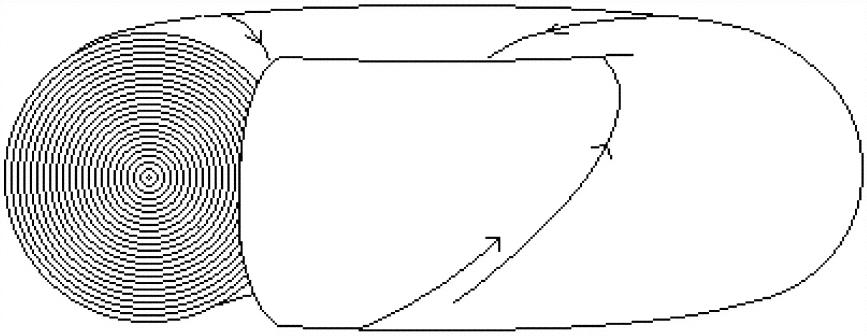
Figure 6. Merely schematic illustration of the invariant tori in an integrable system. A quasiperiodic orbit wraps around a torus filling it densely. The cut-away shows such tori filling the phase space.
A nearly integrable system is a small perturbation of such a system. For example, a Newtonian system of two gravitating bodies is integrable; adding a very small third body produces a nearly integrable system. Such a perturbation can transform some of the invariant tori into much more complicated sets of chaotic orbits, while other tori are only slightly deformed. KAM theory establishes (among other things) sufficient conditions under which a particular torus is only slightly deformed by a perturbation. The deformed invariant tori so established are called the KAM tori. In the case of an n-body system, the orbits that lie on the KAM tori avoid escape and collision; they are stable in the sense of the historic n-body stability problem.
In order for the methods of KAM theory to show that a particular invariant torus survives a perturbation, the torus must meet certain “nonresonance” conditions.Footnote 11 Essentially, the partial derivatives ω i = ∂H 0(p)/∂p i (“frequencies”) of the unperturbed, integrable Hamiltonian H 0(p) on that torus must be far from commensurable, which is usuallyFootnote 12 expressed by a condition of the form
If the function Ω is chosen to grow quickly, the set D of frequency vectors (ω 1, … , ω m) satisfying this condition has positive λ-measure (see De la Llave Reference De la Llave2001). Also, D is nowhere dense, since it is obtained from Rm by removing a small neighborhood around each m-tuple of commensurable frequencies, and such m-tuples are dense. D is therefore riddled, and by Theorem III, u-λ.
Now, D itself is not the union of the KAM tori in the 2m-dimensional phase space. It is a set of m-tuples (ω 1, … , ω m) such that each KAM torus corresponds to an m-tuple in D. However, this correspondence is such as to ensure that the KAM tori are u-λ. Under mild conditions, there exists a diffeomorphism on an open set Tm × P that maps Tm × Ξ ⊆ Tm × P onto the KAM tori, where Tm is the m-dimensional torus, P an open subset of Rm, and Ξ a positive-measure subset of D (Reference JürgenPöschel 1982). Since Tm × Ξ is nowhere dense and diffeomorphisms preserve this property, the union of KAM tori is nowhere dense. Therefore the latter set is riddled, and the KAM theorems state explicitly that it has positive λ-measure. Hence, the KAM tori themselves form a u-λ set (Figure 7).

Figure 7. Schematic cross-section of the invariant tori in a nearly integrable system, showing riddled structure. (In phase spaces with dimension greater than three, orbits are not trapped inside such tori.)
In physical applications, the coordinates (q, p) in which H 0 is independent of q will rarely be the most natural phase space coordinates; it is usually necessary to change variables in order to meet the conditions of KAM theorems. However, the coordinates used in KAM theory are always related to the natural coordinates by “canonical” transformations, which preserve both the topology and the natural measure. Hence, when λ is the natural measure, the KAM tori are riddled, positive-measure, and therefore u-λ even in the natural physical coordinates.
Though these tori form u-λ sets, whether the stability problem itself is u-λ is still an open question. There might be many more stable orbits not on the KAM tori, in which case the set of all orbits that are stable in our sense might not be riddled. However, Reference Arnol’dArnol'd (1964) has constructed examples of orbits of nearly integrable systems that escape, and conjectured that the existence of such orbits is generic. If further almost all orbits not lying on the KAM tori escape, then the positive-measure set of stable orbits is riddled and therefore u-λ, and the stability of the solar system is undecidable in that concrete sense. Similar claims might also hold for other physical problems subject to KAM theory, such as that of the stability of particle trajectories in an accelerator (Moser Reference Moser1978).
Incidentally, it is not hard to see that D is r.a., at least if Ω in (3) is Grzegorczyk-computable and points are coded in a reasonably informative way. The proof idea is just this: To determine with high accuracy whether (ω 1, … , ω m) ∊ D, determine whether (3) holds for a large number of integer m-tuples (j 1, … , j m). Also there should be little difficulty in showing that the KAM tori themselves are r.a. if the relevant transformations are sufficiently computable. Hence again, u-λ characterizes cases of significant undecidability that r.a. obscures.
7. Conclusions
Decidability in a measure μ is a natural relaxation of the concept of decidability, especially in physical contexts. When μ is appropriately chosen, d-μ amounts to the existence of a decision procedure that succeeds with probability one. It is also nontrivial in extension and distinct from other relaxed decidabilities.
We have seen that any riddled set with positive Lebesgue measure is undecidable in λ (Theorem III), though such a set may be r.a. (Theorem IV). It therefore appears that u-λ is just the kind of undecidability that Sommerer and Ott intended to assert in 1996. If they are correct in concluding from the numerical evidence that their example has riddled, positive-measure basins, then those basins are u-λ, though there is good reason to suspect they are nonetheless r.a.
We have also seen that the KAM tori are u-λ, since they too form riddled, positive-measure sets. This suggests that the stability of the solar system, and the qualitative long-term behavior of many other conservative systems, may be undecidable in the concrete sense of u-λ. Whether this is so depends on yet unknown facts, but in any case, the concept of undecidability in a measure μ defined here is one rigorous notion of undecidability that can be meaningfully applied to such problems.
One may raise doubts about the physical significance of undecidability results such as those presented here. The models we have considered are highly idealized and grounded in the out-dated prequantum worldview. In particular, questions about the unbounded future of a model may have no physical meaning, since it is intuitively doubtful that any real system will last forever, or more precisely, retain its form—adhere to one model—forever.
There might still be ways in which some actual physical system could nonetheless behave undecidably in a meaningful sense, but let us not pursue this here. Our primary concern has not been with the occurrence of actual undecidable motion, but with illustrating the concept of decidability in μ. We have not been concerned with the actual solar system, which, due to energy dissipation if nothing else, will no doubt crumble one day. Rather, we have sought to clarify some speculations about a mathematical problem raised by classical physics, and to do so in a manner appropriate to that context. More generally, our results on riddled basins and KAM theory have demonstrated fundamental theoretical difficulties that arise even for the prediction of simple models, long before real-world contingencies are brought to bear—difficulties quite different from chaos and from quantum indeterminacy. We have seen that even if the world were deterministic, classical, susceptible to exact measurement, and well captured by idealized models, some systems could still present significant computational barriers to prediction.
Appendix
Let ||·|| denote the Euclidean norm on Rn. Fix a finite alphabet A and let A* be the set of finite strings from A. Fix a coding N: A* → N onto N, and for each n, a coding Q n: A* → Qn onto Qn, such that the relation ||Q n(s 1) − Q n(s 2)|| ≤ Q n(s 3) is recursive.
Definition 1.
(i) A Cauchy oracle for x is a function φ: A* → A* such that ||Q n(φ(s)) − x|| < 2−N(s) for all s ∊ A*. CO x denotes the set of Cauchy oracles for x.
(ii) When an OTM M is supplied with a particular oracle φ we refer to it as M φ. If M φ halts on an input string s, we write M φ(s)↓ and denote the output string by M φ(s) or M φ(s)↓.
(iii) Let σ : {0, 1, … , k} → A* be a finite sequence of strings. We say that length(σ) = k + 1. For any φ: N → A*, we write σ ⊂ φ and φ ⊃ σ if σ(i) = φ(i) for all i ∊ dom(σ) = {0, 1, … , k}.
(iv) We write M σ(n)↓ = x if for some oracle function φ ⊃ σ, M φ(n)↓ = x and M φ(n) queries the oracle only with numbers in dom(σ)—i.e., M φ never enters the query state with a string s on the oracle tape such that N(s) ≥ length(σ). If no such φ exists, we write M σ(n)↑.
Proposition 1 (Use Principle). M φ(n)↓ = x ⇔ (∃σ ⊂ φ) M σ(n)↓ = x.
Proof. See Soare (Reference Soare1987). ▪
Definition 2. B(x, ∊) (B[x, ∊]) denotes the open (closed) ball with center x and radius ∊.
Theorem I (Topological Use Principle). If M φ(n)↓ = q for some φ ∊ CO x, then there is a neighborhood U of x such that (∀y ∊ U)(∃ψ ∊ CO y) M ψ(n)↓ = q.
Proof. Fix x ∊ Rn and suppose φ satisfies the antecedent. By the Use Principle, choose a finite sequence σ such that σ ⊂ φ and M σ(n)↓ = q. Let U = ∩i ≤ length(σ) B(φ(i), 2–i). To see that U satisfies the consequent, let y ∊ U. Choose θ ∊ CO y and let
Then ψ ∊ CO y, and by the Use Principle, M ψ(n)↓ = M σ(n)↓ = q. ▪

Definition 3. A set B ⊆ Rn is recursively approximable (r.a.) if there is an OTM M such that (∀x ∊ Rn, φ ∊ CO x, m ∊ Z+)(M φ(m)↓ and λ*E M, m(B) ≤ 2–m), where λ* denotes Lebesgue outer measure and E M, m(B) = {x ∊ Rn | (∃φ ∊ CO x) M φ(m) ≠ χ B(x)}.
Definition 4. For any measure μ on Rn, a set B ⊆ Rn is decidable in μ (or d-μ) if there exists an OTM M such that
is μ-measurable and μE M(B) = 0. (The null string ⊘ here is an arbitrary choice.) Otherwise, B is undecidable in μ (or u-μ).Note that without the alternative M φ(⊘)↑ here, only measure-theoretically trivial sets would be d-μ:

Proposition 2. Suppose μ* is a regular outer measure on Rn (i.e., if U ≠ ⊘ is open in the Euclidean topology then μ*U > 0), B ⊆ Rn, M is an OTM, μE M(B) = 0, and (∀x ∊ Rn)(∀φ ∊ CO x) M φ(⊘)↓ ∊ {0, 1}. Then μB = 0 or μ(B C) = 0, where B C = Rn \ B.
Proof. Assume antecedents. Let U = {x | (∃φ ∊ CO x) M φ(⊘)↓ = 1}, V = {x | (∃φ ∊ CO x) M φ(⊘)↓ = 0}. By Theorem I, U and V are open. Since (∀x ∊ Rn)(∀φ ∊ CO x) M φ(⊘)↓ ∊ {0, 1}, U ∪ V = Rn. Since Rn is connected, either U = ⊘, V = ⊘, or U ∩ V ≠ ⊘. But U ∩ V ⊆ E M(B), so μ(U ∩ V) = 0. Since U ∩ V is open and μ* is regular, U ∩ V = ⊘. Therefore U = ⊘ or V = ⊘. Hence B ⊆ E M(B) or B C ⊆ E M(B). Since μE M(B) = 0, either μB = 0 or μ(B C) = 0. ▪
Theorem II. If B ⊆ Rn is d-λ then B is r.a.
Proof. See main text for strategy. Let S: N → A** be an effective enumeration of the finite sequences of strings in A*. Define U(i) as the set of points with Cauchy oracles φ such that S(i) ⊂ φ, i.e., U(i) = ∩j ≤ length(S(i)) B(Q n(S(i)j), 2–j) where S(i)j is the j th string in S(i). Where length(S(i)) = 2j, let V(i) = ∪k ≤ jB(Q n(S(i)2k− 1), Q n(S(i)2k)).
Suppose an OTM M satisfies Definition 4. For each m ∊ N, construct recursive sequences of integers u[m, i], v[m, i] as follows:
1. Set R, i = 1.
2. Simulate M S(j) for all j ∊ N simultaneously (by dovetailing). Whenever M S(j)(⊘)↓ for some j, let u[m, i] = j and i = i + 1. Once λ(B[0, R] \ ∪k≤iU(u[m, k])) < 2–m − R − 1, proceed to 3. (Volumes of finite unions, intersections, and differences of rational balls can be computed to any accuracy, since we assume ||Q n(s 1) − Q n(s 2)|| ≤ Q n(s 3) is recursive.)
3. By trial and error, fix v[m, R] such that λV(v[m, R]) < 2–m − R − 1 and B[0, R] ⊆ ∪j ≤ iU(u[m, j]) ∪ ∪j ≤ R V(v[m, j]). Let R = R + 1 and go to 2.
Each repetition of 2 and 3 will halt because B[0, R] is compact. Note ∪i[U(u[m, i]) ∪ V(v[m, i])] = Rn, and λ∪iV(v[m, i]) < 2–m.
Now an algorithm for a machine M′ satisfying Definition 3 proceeds thus: given input m and oracle φ ∊ CO x, evaluate for each i (again by dovetailing) whether x ∊ U(u[m, i]) and whether x ∊ V(v[m, i]). If x ∊ U(u[m, i]), output M S(u[m, i])(⊘). If x ∊ V(v[m, i]), output 0.
Since ∪i[U(u[m, i]) ∪ V(v[m, i])] = Rn, M′ will halt on every Cauchy oracle. Also, E M′, m(B) ⊆ E M(B) ∪ ∪iV(v[m, i]). Since λE M(B) = 0 and λ∪iV(v[m, i]) < 2–m, λE M′, m(B) < 2–m. ▪
Definition 5. A set B ⊆ Rn is riddled if for every open set U ≠ ⊘ in the Euclidean topology, λ*(U \B) > 0.
Theorem III. If B ⊆ Rn is riddled and λ*B > 0, then B is u-λ.
Proof. Assume the antecedents and suppose M is an OTM. We show that λ*E M(B) > 0.
Case 1:¬(∃x ∊ Rn)(∀φ ∊ CO x) M φ(⊘) = 1. Then E M(B) ⊇ B, so λ*E M(B) ≥ λ*B > 0.
Case 2:(∃x ∊ Rn)(∀φ ∊ CO x) M φ(⊘) = 1. Then by Theorem I, there is a neighborhood U of x such that (∀y ∊ U)(∃ψ ∊ CO y) M ψ(⊘)↓ = 1. Therefore U \B ⊆ E M(B). But by riddling, λ*(U \B) > 0. Therefore λ*E M(B) > 0, so B is u-λ. ▪
Theorem IV. There exists a subset of R that is r.a. but not d-λ.
Proof. Say a closed interval I is maximal in a set S ⊆ R if I ⊆ S and for every closed interval J ⊆ S, J ∩ I ≠ ⊘ ⇒ J ⊆ I. We construct a generalized Cantor set C as follows:
(i) Let C 0 = [0, 1].
(ii) For each i ∊ Z+, let C i = C i − 1\∪{B([a + b]/2, 2–i − 1[b − a]) | [a, b] is maximal in C i− 1}.
(iii) Let C = ∩iC i.
We show that λC > 0. Since the C iare all measurable, λC = 1 − ∑i λ(C i− 1\C i). Our construction (ii) removes the middle (2i)th part from each component of C i− 1. Therefore, λ(C i− 1\C i) = 2–iλC i− 1 ≤ 2–i, with strict inequality for i > 1. So ∑iλ(C i – 1\ C i) < ∑i 2–i = 1. Thus λC > 0. By Theorem III, C is u-λ.
We now show that C is r.a. by sketching an OTM that approximates C. The algorithm is this: given input m, let M φ request from its oracle φ the value of φ(2m + 3), and determine whether the Q[φ(2m + 3)] is in C m+1. (This can be done effectively since one can construct the rational endpoints of C m+1 following (i)-(iii), and we code rationals so that |q 1 − q 2| ≤ q 3 is recursive.) If Q[φ(2m + 3)] ∊ C m+1, let M φ(m) = 1; otherwise M φ(m) = 0.
Since |Q[φ(2m + 3)] − x| < 2–(2m+3) any x ∊ E M, m(C m+1) must be close to one of the 2m+2 endpoints of C m+1, within distance 2–(2m+3). Therefore λ*E M, m(C m+1) ≤ (2m+2)(2–(2m+3)) = 2–(m+1). So, if λ(C m+1\C) ≤ 2–(m+1), then λ*E M, m(C) ≤ 2–(m+1) + 2–(m+1) = 2–m. This is in fact the case, for we now show that for all i, λ(C i\C) < 2–i. For i = 0 we have λ(C 0\C) = λC 0 − λC < 1 = 20, since λC > 0. For i > 0 we have λ(C i\C) = Σj > i λ(C j− 1 − C j) = (by construction) Σj > i 2−jλC j− 1 < Σj > i 2−j = 2−i. Therefore λ*E M, m(C) ≤ 2–m, so C is r.a. ▪


