


1. Introduction
This work is focused on the description of flow fields in porous media which occur in many applications, such as groundwater and oil flows, industrial filtering processes or in transpiration cooling (van Foreest et al. Reference van Foreest, Glhan, Esser, Sippel, Ambrosius and Sudmeijer2020). The emphasis of the current work is on transpiration cooling applications, but could be applied to any analogous porous flow problem. Transpiration cooling is defined as the passing of a relatively cool fluid through a porous medium in order to protect it from a high enthalpy external flow (Rubesin Reference Rubesin1954). This type of active cooling approach is envisioned for future hypersonic vehicles, such as re-entry capsules, space planes or scramjet powered wave riders (Esser et al. Reference Esser, Gülhan, Reimer and Petkov2015). All of those vehicles travel through the atmosphere at very high speeds of several kilometres per second. This leads to a strong compression shock in front of them in which the large kinetic energy is partially transferred into internal energy of the surrounding gas (Anderson Reference Anderson2006). The resulting post-shock flow field leads to an extreme surface heat flux that needs to be mitigated in order to ensure survival of the vehicle. The aforementioned cooling technique of transpiration through a porous external skin of the vehicle can reduce heat fluxes significantly to make them manageable for existing materials (Boehrk, Piol & Kuhn Reference Boehrk, Piol and Kuhn2010; Liu et al. Reference Liu, Jiang, Jin and Sun2010).
The external flow field around the porous wall can exhibit large lateral gradients in surface heat flux and pressure. This is exacerbated for a slender vehicle when the leading edge radius becomes small, as the surface pressure and heat transfer become concentrated on the stagnation point and the downstream flow field will approximate the post-shock state after an oblique shock wave (Lees Reference Lees1956). This situation requires a spatial distribution of transpired coolant that is higher at the stagnation point and falls off toward the downstream region (Hermann, McGilvray & Naved Reference Hermann, McGilvray and Naved2020). Designed distributed blowing is further complicated through the changing external surface pressure, which will impose an internal flow pattern in the porous medium. In addition, changing wall thickness and impermeable sections can be present in the design of the porous surface. Thinner wall sections are used to drive more coolant mass flux in regions where significant blowing is required and a large external surface pressure is acting on the vehicle. As the plenum side of the porous medium has to be connected to the internal structure of the vehicle, some regions behind the porous surface will be impermeable to coolant (Boehrk & Beyermann Reference Boehrk and Beyermann2010). All these factors lead to a complicated flow field inside the porous domain. To aid the design and evaluation process of appropriate porous structures, an analytical description of the flow field is highly useful. The derivation and validation of such a formulation is the topic this work.
The two-dimensional flows in porous media have been extensively studied using potential flow theory in e.g. Sherwood & Stone (Reference Sherwood and Stone2001), Ding & Wang (Reference Ding and Wang2018), Warrick, Broadbridge & Lomen (Reference Warrick, Broadbridge and Lomen1992) and Nguyen & Raudkivi (Reference Nguyen and Raudkivi1983), which allows for closed analytical descriptions of the potential and streamfunctions, respectively. The resulting mathematical boundary value problem can then be applied to the respective cases to determine a function for the pressure and velocity fields. For homogeneous Dirichlet (pressure) or Neumann (velocity) boundary condition problems, the solution is straightforward. Mixed Dirichlet–Neumann boundary conditions, however, pose more challenging to solve analytically, as the usually employed orthogonality conditions fail. In this case, a different mathematical approach is required, e.g. an iterative scheme, such as shown in Read (Reference Read2000). The current work contributes to the existing literature by building on the method developed in Read (Reference Read2007) and extends the mixed Neumann–Dirichlet problem to a generalised case by accounting for an additional external boundary condition of arbitrary shape. In this work, these formulations will be derived both for Cartesian and cylindrical coordinate systems, which are appropriate for flows in flat plates and curved geometries, respectively. The current work provides engineering level tools using pressure as boundary conditions which are useful as a first-order design step. The pressure boundary condition on the external flow side can be extracted from various sources, such as computational fluid dynamics simulations or semi-empirical correlations. This procedure is valid if the injected mass flux is small compared to the mass flux of the external flow and hence does not significantly alter the external flow field. Please note that the analysis provided in this work does not include higher-order effects, e.g. slip, transpiration and resistance coefficients, occurring at the external flow interface as described in Beavers & Joseph (Reference Beavers and Joseph1967), Carraro et al. (Reference Carraro, Goll, Marciniak-Czochra and Mikeli2013), Lācis et al. (Reference Lācis, Sudhakar, Pasche and Bagheri2020) and Rife & di Mare (Reference Rife and di Mare2019). The pressure and velocity fields derived in this work can be used as a boundary condition in combination with a numerical simulation of the external flow field and an appropriate interface model.
2. Potential flow description of porous domain
The fundamental laws describing a steady state incompressible flow in a homogeneous isotropic porous medium are Darcy's law,
 \begin{equation} \boldsymbol{u} ={-} \frac{K_D}{\mu} \boldsymbol{\nabla} p,\end{equation}
and the incompressible continuity equation,
 \begin{equation} \boldsymbol{\nabla} \boldsymbol{\cdot} \boldsymbol{u} = 0,\end{equation}
with the velocity vector  $\boldsymbol {u}$, the pressure
  $p$, the dynamic viscosity
  $\mu$ and the permeability
  $K_D$ (Nield & Bejan Reference Nield and Bejan2012). A scalar potential function
  $\varPhi$ can be defined by
 \begin{equation} \boldsymbol{u} = \boldsymbol{\nabla} \varPhi.\end{equation}
Under the assumption of a homogeneous and isotropic porous medium, (2.3) relates to the pressure field through (2.1) as
 \begin{equation} p ={-} \frac{\mu}{K_D} \varPhi,\end{equation}
and relates to the velocity field in Cartesian coordinates through (2.3) by
 \begin{equation} v_x = \frac{\partial \varPhi}{\partial x}, \quad v_y = \frac{\partial \varPhi}{\partial y},\end{equation}
with the velocity in the horizontal ( $x$) direction
  $v_x$, and the velocity in the vertical (
 $y$) direction
  $v_y$. In cylindrical coordinates, the respective velocities are
 \begin{equation} v_{\theta} = \frac{1}{r} \frac{\partial \varPhi}{\partial \theta}, \quad v_r = \frac{\partial \varPhi}{\partial r},\end{equation}
with the velocity in the angular ( $\theta$) direction
  $v_{\theta }$, and the velocity in the radial (
 $r$) direction
  $v_r$. Combining (2.2) and (2.3) yields Laplace's equation
 \begin{equation} \nabla^2 \varPhi = 0.\end{equation}
In addition, a corresponding streamfunction  $\varPsi$ is defined through the Cauchy–Riemann equations in Cartesian coordinates,
 \begin{equation} \frac{\partial \varPhi}{\partial x} = \frac{\partial \varPsi}{\partial y} \quad \mathrm{and} \quad \frac{\partial \varPhi}{\partial y} ={-} \frac{\partial \varPsi}{\partial x}, \end{equation}
and in cylindrical coordinates,
 \begin{equation} \frac{1}{r} \frac{\partial \varPhi}{\partial \theta} = \frac{\partial \varPsi}{\partial r} \quad \mathrm{and} \quad \frac{\partial \varPhi}{\partial r} ={-} \frac{1}{r} \frac{\partial \varPsi}{\partial \theta}. \end{equation}
3. Solution of Laplace's equation
This section details the mathematical derivation of the solutions to (2.7) for the two investigated cases of Cartesian and cylindrical coordinate systems.
3.1. Cartesian coordinates
The general solution of (2.7) in Cartesian coordinates can be obtained through a separation of variables and yields
 \begin{equation} \varPhi(x,y) = a + b y + ( \alpha \cos (\lambda x) + \beta \sin(\lambda x) ) ( \delta \cosh (\lambda y) + \gamma \sinh (\lambda y) ), \end{equation}
with the constants  $a$,
$a$,  $b$,
$b$,  $\alpha$,
  $\beta$,
  $\delta$,
  $\gamma$ and
  $\lambda$ which have to be determined from specific boundary conditions. The porous domain, sketched in figure 1, starts at
  $x=y=0$ in the left bottom corner, and has a width of
  $d$ and a height of
  $t$. Boundaries 1 and 2 are vertical and represent the end of the porous domain in the horizontal direction. Boundary 3 represents the interface to an external flow field where an arbitrary pressure distribution
  $p_e(x)$ can be present. Boundary 4 is on the plenum side and can have any arbitrary thickness distribution
  $b_i(x)$. Any plenum pressure distribution
  $p_i(x)$ is possible, and this side can have a number of impermeable segments along this boundary (figure 1 only shows a single one for clarity). These boundary conditions can be represented mathematically as follows: the left and right boundary conditions are represented as impermeable conditions
 \begin{gather} \text{Boundary 1:} \ \frac{\partial \varPhi}{\partial x}(0,y)= 0, \end{gather}
 \begin{gather}\text{Boundary 2:} \ \frac{\partial \varPhi}{\partial x}(d,y)= 0, \end{gather}
which can also be interpreted as a symmetrical boundary. The interface to the external flow field has the pressure boundary condition
 \begin{equation} \text{Boundary 3:}\ \varPhi(x,t)= \varPhi_e(x) ={-} \frac{K_D}{\mu} p_e(x). \end{equation}
The plenum boundary is a mixed case of Dirichlet and Neumann boundary conditions. At permeable locations, the flow in the porous medium is driven by a pressure  $p_i(x)$ which can vary along the horizontal axis. At impermeable locations, no flow can cross the boundary
  $b_i(x)$. This is mathematically described as
 \begin{equation} \text{Boundary 4:} \ \left. \begin{array}{ll@{}} \displaystyle \varPhi(x,b_i(x))=\varPhi_i(x) ={-} \dfrac{K_D}{\mu} p_i(x) & \mbox{for permeable locations,}\\ \displaystyle \varPsi(x,b_i(x)) = \varPsi_i = \mbox{const.} & \mbox{for impermeable locations.\ } \end{array}\right\}\end{equation}
Using (3.2) and (3.3) in (3.1) yields the intermediate solution
 \begin{equation} \varPhi(x,y) = a + b y + \sum_{n=1}^{\infty} ( \delta_n \cosh (N y) + \gamma_n \sinh (N y) ) \cos (N x) \quad \mbox{with\ } N = \frac{{\rm \pi} n}{d}. \end{equation}
An infinite sum of solutions has been constructed, where each individual term, i.e. for each  $n$, fulfils (2.7). Due to the linearity of Laplace's equation, these can be superimposed, which is required in the next step when accounting for the internal and external boundary conditions. The external potential is expressed as the Fourier series
 \begin{align} \varPhi_e(x) &= \frac{A_0}{2} + \sum_{n=1}^{\infty} A_n \cos (Nx) \mbox{ with} \ A_0 = \frac{2}{d} \int_{0}^{d} \varPhi_e(x) \,\mbox{d}x \mbox{ and}\notag\\ A_n &= \frac{2}{d} \int_{0}^{d} \varPhi_e(x) \cos (Nx) \,\mbox{d}x .\end{align}
Using a term-by-term coefficient comparison between (3.6) and (3.7), each coefficient  $A_n$ can be related to the respective coefficients
  $\delta _n$,
  $\gamma _n$,
  $a$ and
  $b$ by
 \begin{equation} \delta_n \cosh (N t) + \gamma_n \sinh (N t) = \frac{2}{d} \int_{0}^{d} \varPhi_e(x) \cos (Nx) \,\mbox{d}x, \end{equation}
and
 \begin{equation} a + b t = \frac{1}{d} \int_{0}^{d} \varPhi_e(x) \,\mbox{d}x,\end{equation}
yielding the solution
 \begin{align} \varPhi(x,y) & = \frac{1}{d} \int_{0}^{d} \varPhi_e(x)\,\mbox{d}x + B_0(y-t) \nonumber\\ & \quad + \sum_{n=1}^{\infty} B_n ( \cosh (N y) -\coth (N t) \sinh (N y) ) \cos (N x) \nonumber\\ & \quad + \sum_{n=1}^{\infty} \frac{\displaystyle\frac{2}{d} \int_{0}^{d} \varPhi_e(x) \cos (Nx) \,\mbox{d}x}{\sinh (N t)} \sinh (N y) \cos (N x). \end{align}
For convenience, in the following derivation, the constants  $b$ and
  $\delta _n$ have been relabelled as
  $B_0$ and
  $B_n$, respectively. The corresponding streamfunction can be obtained via the Cauchy–Riemann equations ((2.8a,b)) as
 \begin{align} \varPsi(x,y) & = B_{{-}1} - B_0 x - \sum_{n=1}^{\infty} B_n ( \sinh (N y) -\coth (N t) \cosh (N y) ) \sin(N x) \nonumber\\ &\quad - \sum_{n=1}^{\infty} \frac{\displaystyle\frac{2}{d} \int_{0}^{d} \varPhi_e(x) \cos (Nx) \,\mbox{d}x}{\sinh (N t)} \cosh (N y) \sin(N x), \end{align}
with the arbitrary constant  $B_{-1}$ which stems from an indefinite integral. The remaining unknown coefficients
  $B_n$ are determined from the internal boundary condition by employing and expanding on the methodology developed in Read (Reference Read2007). The boundary forcing function
  $F(x)$ is defined as
 \begin{equation} F(x) = \left\{
\begin{array}{@{}ll} \displaystyle\varPhi_i(x) -
\dfrac{1}{d} \int_{0}^{d} \varPhi_e(x)\,\mbox{d}x
\\ \quad - \displaystyle \sum_{n=1}^{\infty}
\dfrac{\displaystyle\dfrac{2}{d} \int_{0}^{d} \varPhi_e(x)
\cos (Nx) \,\mbox{d}x}{\sinh (N t)} \sinh (N b_i(x)) \cos
(N x), & \mbox{perm.}\\
\displaystyle\varPsi_i + \sum_{n=1}^{\infty}
\dfrac{\displaystyle\dfrac{2}{d} \int_{0}^{d} \varPhi_e(x)
\cos (Nx) \,\mbox{d}x}{\sinh (N t)} \cosh (N b_i(x)) \sin(N
x). & \mbox{imperm}. \end{array} \right.
\end{equation}
\begin{equation} F(x) = \left\{
\begin{array}{@{}ll} \displaystyle\varPhi_i(x) -
\dfrac{1}{d} \int_{0}^{d} \varPhi_e(x)\,\mbox{d}x
\\ \quad - \displaystyle \sum_{n=1}^{\infty}
\dfrac{\displaystyle\dfrac{2}{d} \int_{0}^{d} \varPhi_e(x)
\cos (Nx) \,\mbox{d}x}{\sinh (N t)} \sinh (N b_i(x)) \cos
(N x), & \mbox{perm.}\\
\displaystyle\varPsi_i + \sum_{n=1}^{\infty}
\dfrac{\displaystyle\dfrac{2}{d} \int_{0}^{d} \varPhi_e(x)
\cos (Nx) \,\mbox{d}x}{\sinh (N t)} \cosh (N b_i(x)) \sin(N
x). & \mbox{imperm}. \end{array} \right.
\end{equation}
In addition, the coefficient function  $U_n(x)$ is defined as
 \begin{equation} U_{n}(x) = \left\{ \begin{array}{@{}ll} ( \cosh (N b_i(x)) -\coth (N t) \sinh (N b_i(x)) ) \cos (N x) , & \mbox{permeable} \\ - ( \sinh (N b_i(x)) -\coth (N t) \cosh (N b_i(x)) ) \sin(N x), & \mbox{impermeable}, \end{array} \right.\end{equation}
with
 \begin{equation} U_{0}(x) = \left\{ \begin{array}{@{}ll} b_i(x) - t , & \mbox{permeable} \\ - x, & \mbox{impermeable}, \end{array} \right. \end{equation}
and
 \begin{equation} U_{{-}1}(x) = \left\{ \begin{array}{@{}ll} 0, & \mbox{permeable} \\ 1, & \mbox{impermeable}. \end{array} \right. \end{equation}
These functions allow the expression of (3.5) as
 \begin{equation} F(x) = \sum_{n={-}1}^{M} B_n U_n(x).\end{equation}
Here, the Fourier series is truncated to  $M+2$ terms corresponding to the coefficients
  $B_{n}$ for
  $n = -1,0,1,\ldots ,M$. Following on from the work in Read (Reference Read2007), the normal equations of this problem are
 \begin{equation} \sum_{j={-}1}^{M} B_j \int_{0}^{d} U_i(x) U_j(x)\, \mathrm{d} x = \int_{0}^{d} U_i(x) F(x)\, \mathrm{d} x,\end{equation}
which can also be represented in a matrix form as
 \begin{equation} \boldsymbol{U} \boldsymbol{\cdot} \boldsymbol{b} = \boldsymbol{f},\end{equation}
with the matrix entries for  $\boldsymbol {U}$,
 \begin{equation} [\boldsymbol{U}]_{ij} = \int_{0}^{d} U_i(x) U_j(x)\, \mathrm{d} x ,\end{equation}
the vector entries for  $\boldsymbol {f}$,
 \begin{equation} [\boldsymbol{f}]_{i} = \int_{0}^{d} U_i(x) F(x)\, \mathrm{d} x ,\end{equation}
and the entries of the unknown coefficients’ vector  $\boldsymbol {b}$,
 \begin{equation} [\boldsymbol{b}]_{i} = B_i .\end{equation}
Equations (3.19) and (3.20) can be solved with any appropriate numerical method. In the cases presented in § 5, the integrals have been solved using trapezoidal integration. Equation (3.18) can simply be solved by
 \begin{equation} \boldsymbol{b} = \boldsymbol{U}^{{-}1} \boldsymbol{\cdot} \boldsymbol{f},\end{equation}
to yield the remaining coefficients  $B$. Equation (3.22) is valid for a square matrix of size
  $M+2 \times M+2$. Alternatively, the matrix can be rectangular and of the size
  $M+2 \times \tilde {M}$, which results in the solution
 \begin{equation} \boldsymbol{U}^\textrm{T} \boldsymbol{U} \boldsymbol{b} = \boldsymbol{U}^\textrm{T} \boldsymbol{\cdot} \boldsymbol{f}. \end{equation}
This over collocation method has been shown to work best with  $\tilde {M} = 2M$ to
  $5M$ points (Read Reference Read2007). For convenience, the resulting formulations for the pressure field
  $p(x,y)$, velocity components
  $v_x(x,y)$,
  $v_y(x,y)$ and the streamfunction
  $\varPsi (x,y)$ are given below in terms of the original pressure boundary conditions. Pressure field
 \begin{align} p(x,y) & = \frac{1}{d} \int_{0}^{d} p_e(x)\,\mbox{d}x - \frac{\mu}{K_D} B_0(y-t) \nonumber\\ &\quad - \frac{\mu}{K_D} \sum_{n=1}^{M} B_n ( \cosh (N y) -\coth (N t) \sinh (N y) ) \cos (N x) \nonumber\\ & \quad + \sum_{n=1}^{M} \frac{\displaystyle\frac{2}{d} \int_{0}^{d} p_e(x) \cos (Nx) \,\mbox{d}x}{\sinh (N t)} \sinh (N y) \cos (N x) , \end{align}
velocity components
 \begin{align} v_x(x,y) &={-} \sum_{n=1}^{M} B_n N ( \cosh (N y) -\coth (N t) \sinh (N y) ) \sin(N x) \nonumber\\ & \quad + \frac{K_D}{\mu} \sum_{n=1}^{M} N \frac{\displaystyle\frac{2}{d} \int_{0}^{d} p_e(x) \cos (Nx) \,\mbox{d}x}{\sinh (N t)} \sinh (N y) \sin(N x) ,\end{align}
 \begin{align} v_y(x,y) & = B_0 + \sum_{n=1}^{M} B_n N ( \sinh (N y) -\coth (N t) \cosh (N y) ) \cos (N x)\notag\\ &\quad - \frac{K_D}{\mu} \sum_{n=1}^{M} N \frac{\displaystyle\frac{2}{d} \int_{0}^{d} p_e(x) \cos (Nx) \,\mbox{d}x}{\sinh (N t)} \cosh (N y) \cos (N x) , \end{align}
and streamfunction
 \begin{align} \varPsi(x,y) & = B_{{-}1} - B_0 x - \sum_{n=1}^{M} B_n ( \sinh (N y) -\coth (N t) \cosh (N y) ) \sin(N x) \nonumber\\ & \quad + \frac{K_D}{\mu} \sum_{n=1}^{M} \frac{\displaystyle\frac{2}{d} \int_{0}^{d} p_e(x) \cos (Nx) \,\mbox{d}x}{\sinh (N t)} \cosh (N y) \sin(N x), \end{align}
with  $N = ({\rm \pi} n )/d$.

Figure 1. Sketch of mathematical domain in Cartesian coordinates. White areas denote porous material, while shaded areas denote impermeable material.
3.2. Cylindrical coordinates
The derivation of the solution in cylindrical coordinates is analogous to the previous section. Therefore, only the main steps will be shown. The general solution of (2.7) in cylindrical coordinates is
 \begin{equation} \varPhi(\theta,r) = a + b\ln (r) + ( \alpha \cos (\lambda \theta) + \beta \sin(\lambda \theta) ) ( \delta r^{-\lambda} + \gamma r^{\lambda} ). \end{equation}
The respective porous domain is shown in figure 2 and resembles an architecture which would be found in a porous leading edge of a hypersonic vehicle (Colwell & Modlin Reference Colwell and Modlin1992). The porous domain extends from  $\theta =0$ to
  $s$, where it is terminated by an impermeable boundary in radial orientation, and the domain is symmetrical along the
  $\theta =0$ axis. Similarly to the Cartesian case, the external boundary is given by a pressure distribution
  $p_e(\theta )$ at the external radius
  $R_e$. The internal boundary can have an arbitrary shape
  $R_i(\theta )$, and can feature permeable and impermeable sections. Theses boundary conditions can be expressed as
 \begin{gather} \text{Boundary 1:} \ \frac{\partial \varPhi}{\partial \theta}(0,r)= 0, \end{gather}
 \begin{gather}\text{Boundary 2:} \ \frac{\partial \varPhi}{\partial \theta}(s,r)= 0, \end{gather}
 \begin{gather}\text{Boundary 3:}\ \varPhi(\theta,R_e)= \varPhi_e(\theta) ={-} \frac{K_D}{\mu} p_e(\theta), \end{gather}
 \begin{gather}\text{Boundary 4:} \ \left. \begin{array}{ll@{}} \displaystyle \varPhi(\theta,R_i(\theta))=\varPhi_i(\theta) ={-} \dfrac{K_D}{\mu} p_i(\theta) & \mbox{for permeable locations,}\\ \displaystyle \varPsi(\theta,R_i(\theta)) = \varPsi_i = \mbox{const.} & \mbox{for impermeable locations.} \end{array}\right\} \end{gather}
Implementing boundary conditions 1–3 yields the potential function
 \begin{align} \varPhi(\theta,r) & = \frac{1}{s} \int_{0}^{s} \varPhi_e(\theta)\,\mbox{d}\theta + B_0 \ln \left(\frac{r}{R_e}\right) + \sum_{n=1}^{\infty} B_n ( r^{{-}N} -R_e^{{-}2N} r^N ) \cos (N \theta) \nonumber\\ & \quad +\sum_{n=1}^{\infty} \left(\frac{r}{R_e}\right)^N \cos(N \theta) \frac{2}{s} \int_{0}^{s} \varPhi_e(\theta) \cos (N\theta) \,\mbox{d}\theta , \end{align}
and the streamfunction
 \begin{align} \varPsi(\theta,r) & = B_{{-}1} - B_0 \theta + \sum_{n=1}^{\infty} B_n ( r^{{-}N} + R_e^{{-}2N} r^N ) \sin(N \theta) \nonumber\\ &\quad - \sum_{n=1}^{\infty} \left(\frac{r}{R_e}\right)^N \sin(N \theta) \frac{2}{s}\int_{0}^{s} \varPhi_e(\theta) \cos (N\theta) \,\mbox{d}\theta. \end{align}
In order to account for boundary condition 4, the following functions are defined. The forcing function
 \begin{equation} F(x) = \left\{
\begin{array}{@{}ll} \displaystyle\varPhi_i(\theta) -
\dfrac{1}{s} \int_{0}^{s} \varPhi_e(\theta)\,\mbox{d}\theta
\\ \quad - \displaystyle \sum_{n=1}^{\infty}
\left(\dfrac{R_i(\theta)}{R_e}\right)^N \cos(N
\theta)\dfrac{2}{s} \int_{0}^{s} \varPhi_e(\theta) \cos
(N\theta) \,\mbox{d}\theta, & \mbox{perm.}
\\ \displaystyle\varPsi_i +
\sum_{n=1}^{\infty} \left(\dfrac{R_i(\theta)}{R_e}\right)^N
\sin(N \theta) \dfrac{2}{s} \int_{0}^{s} \varPhi_e(\theta)
\cos (N\theta) \,\mbox{d}\theta, & \mbox{imperm}.
\end{array} \right.\end{equation}
\begin{equation} F(x) = \left\{
\begin{array}{@{}ll} \displaystyle\varPhi_i(\theta) -
\dfrac{1}{s} \int_{0}^{s} \varPhi_e(\theta)\,\mbox{d}\theta
\\ \quad - \displaystyle \sum_{n=1}^{\infty}
\left(\dfrac{R_i(\theta)}{R_e}\right)^N \cos(N
\theta)\dfrac{2}{s} \int_{0}^{s} \varPhi_e(\theta) \cos
(N\theta) \,\mbox{d}\theta, & \mbox{perm.}
\\ \displaystyle\varPsi_i +
\sum_{n=1}^{\infty} \left(\dfrac{R_i(\theta)}{R_e}\right)^N
\sin(N \theta) \dfrac{2}{s} \int_{0}^{s} \varPhi_e(\theta)
\cos (N\theta) \,\mbox{d}\theta, & \mbox{imperm}.
\end{array} \right.\end{equation}
and the coefficient function
 \begin{equation} U_{n}(\theta) = \left\{ \begin{array}{@{}ll} ( R_i(\theta)^{{-}N} -R_e^{{-}2N} R_i(\theta)^N ) \cos (N \theta), & \mbox{permeable}, \\ ( R_i(\theta)^{{-}N} +R_e^{{-}2N} R_i(\theta)^N ) \sin(N \theta), & \mbox{impermeable}, \end{array} \right.\end{equation}
with
 \begin{equation} U_{0}(\theta) = \left\{ \begin{array}{@{}ll} \ln \left(\dfrac{R_i(\theta)}{R_e}\right) , & \mbox{permeable} \\ - \theta, & \mbox{impermeable}, \end{array} \right.\end{equation}
and
 \begin{equation} U_{{-}1}(\theta) = \left\{ \begin{array}{@{}ll} 0, & \mbox{permeable}, \\ 1, & \mbox{impermeable}. \end{array} \right.\end{equation}
With these functions defined, the steps from (3.16) to (3.22) have to be carried out to obtain the unknown coefficients  $B_n$. The resulting formulations for the pressure field
  $p(\theta ,r)$, velocity components
  $v_{\theta }(\theta ,r)$,
  $v_r(\theta ,r)$ and the streamfunction
  $\varPsi (\theta ,r)$ are given below in terms of the original pressure boundary conditions. Pressure field
 \begin{align} p(\theta,r) & = \frac{1}{s} \int_{0}^{s} p_e(\theta)\,\mbox{d}\theta - \frac{\mu}{K_D} B_0 \ln \left(\frac{r}{R_e}\right) - \frac{\mu}{K_D} \sum_{n=1}^{M} B_n ( r^{{-}N} -R_e^{{-}2N} r^N ) \cos (N \theta)\nonumber\\ & \quad + \sum_{n=1}^{M} \left(\frac{r}{R_e}\right)^N \cos(N \theta)\frac{2}{s} \int_{0}^{s} p_e(\theta) \cos (N\theta) \,\mbox{d}\theta , \end{align}
velocity components
 \begin{align} v_{\theta}(\theta,r) &={-} \sum_{n=1}^{M} B_n N ( r^{{-}N-1} -R_e^{{-}2N} r^{N-1} ) \sin(N \theta) \nonumber\\ & \quad +\frac{K_D}{\mu} \sum_{n=1}^{M} \frac{r^{N-1}}{R_e^N} N \sin (N \theta) \frac{2}{s} \int_{0}^{s} p_e(\theta) \cos (N\theta) \,\mbox{d}\theta , \end{align}
 \begin{align} v_r(\theta,r) & = B_0 \frac{1}{r} - \sum_{n=1}^{M} B_n N ( r^{{-}N-1} +R_e^{{-}2N} r^{N-1} ) \cos (N \theta) \nonumber\\ &\quad -\frac{K_D}{\mu} \sum_{n=1}^{M} \frac{r^{N-1}}{R_e^N} N \cos (N \theta) \frac{2}{s} \int_{0}^{s} p_e(\theta) \cos (N\theta) \,\mbox{d}\theta , \end{align}
and streamfunction
 \begin{align} \varPsi(\theta,r) & = B_{{-}1} - B_0 \theta + \sum_{n=1}^{M} B_n ( r^{{-}N} + R_e^{{-}2N} r^N ) \sin(N \theta) \nonumber\\ & \quad +\frac{K_D}{\mu} \sum_{n=1}^{M} \left(\frac{r}{R_e}\right)^N \sin(N \theta) \frac{2}{s}\int_{0}^{s} \varPhi_e(\theta) \cos (N\theta) \,\mbox{d}\theta, \end{align}
with  $N = ({\rm \pi} n )/s$.

Figure 2. Sketch of the mathematical domain in cylindrical coordinates. White areas denote porous material, shaded areas denote impermeable material and dashed lines denote symmetry.
4. Mass injection at external boundary
For a transpiration cooling application, the most important quantity to be extracted from these formulations is the outflow distribution at the external boundary condition. This is the driving mass flux that leads to the cooling of the vehicle surface and is the desired quantity in any design process of porous architectures. This outflow velocity is represented by  $v_y$ and
  $v_r$ and can be obtained by inserting the external boundary location
  $y=t$ and
  $r=R_e$ into (3.26) and (3.41), respectively. This simplifies the formulation significantly and results in
 \begin{align} v_y(x,t) &= B_0 - \sum_{n=1}^{M} \frac{B_n N}{\sinh (N t)} \cos(N x)\notag\\ &\quad - \frac{K_D}{\mu} \sum_{n=1}^{M} N \coth (N t) \cos (N x) \frac{2}{d} \int_{0}^{d} p_e(x) \cos (Nx) \,\mbox{d}x , \end{align}
with  $N = ({\rm \pi} n )/d$ for Cartesian coordinates. The resulting outflow velocity in cylindrical coordinates is
 \begin{align} v_r(\theta,R_e) = \frac{B_0}{r} - \sum_{n=1}^{M} \frac{2 B_n N}{ r^{N+1}} \cos (N \theta) - \frac{K_D}{\mu} \sum_{n=1}^{M} \frac{N}{r} \cos (N \theta) \frac{2}{s} \int_{0}^{s} p_e(\theta) \cos (N\theta) \,\mbox{d}\theta ,\end{align}
with  $N = ({\rm \pi} n )/s$. The derived velocities in (4.1) and (4.2) correspond to the Darcy velocity just below the interface between porous domain and external flow. In a subsequent step, these velocities could be used to account for the interface between porous domain and external flow by using a flow resistance model (Idelchik Reference Idelchik1986) or a more complex interface model (Rife & di Mare Reference Rife and di Mare2019; Lācis et al. Reference Lācis, Sudhakar, Pasche and Bagheri2020).
5. Verification examples
This section provides two examples, representing a flat plate and a round leading edge porous structure. The purpose of this section is to illustrate the obtained analytical results for a real case and to verify them by comparing the results to numerical simulations.
5.1. Porous flow in flat plate domain
Figure 3 shows a sketch of the porous domain. A porous flat plate of width  $d=12$ mm and thickness
  $t=2$ mm is bounded left and right by impermeable materials. The domain features a linearly decreasing wall thickness from
  $b_i(x=6\ \mbox {mm})=0$ mm to
  $b_i(x=12\ \mbox {mm})=0.67$ mm. The plenum side is separated into two chambers where a constant pressure of
  $4$ bar is applied from
  $x=0$ mm to
  $3$ mm, and a constant pressure of
  $1.5$ bar is applied from
  $x=6$ mm to
  $12$ mm. The space between these domains is occupied by an impermeable boundary. The top side of the plate is subjected to a pressure boundary that decreases nonlinearly from
  $1.5$ bar to
  $0.75$ bar over the length of the plate and is described by
 \begin{equation} p_e(x) = 1.5\cdot 10^5 \frac{d}{x + d} \ \mathrm{Pa}.\end{equation}
The porous material features a permeability of  $K_D=2.5\cdot 10^{-14}$ m
 $^2$, and the fluid features a dynamic viscosity of
  $\mu =1.5\cdot 10^{-5}\ \textrm {Pa}\cdot \textrm {s}$. The resulting pressure and velocity fields are shown in figure 4 which have been determined by evaluating (3.24)–(3.26), where the absolute velocity is determined as
 \begin{equation} v(x,y) = \sqrt{v_x(x,y)^2 + v_y(x,y)^2}.\end{equation}
The value of the computed Fourier coefficients  $M$ in this case was 80. A comprehensive study of the error in each term for different values of
  $M$ can be found in Read (Reference Read2007). The high pressure boundary between
  $x=0$ and
  $3$ mm on the plenum side is the main driving feature in the pressure distribution. The behaviour between
  $x=0$ and
  $2$ mm approximates a one-dimensional flow in the
  $y$-direction as the change in external pressure over this region is small. Significant edge effects are visible in the vicinity of the pressure-impermeability boundary at
  $x=3$ mm. The velocity distribution clearly shows this boundary between different domains as peaks in the field. Both the left (
 $x=3$ mm) and the right (
 $x=6$ mm) boundaries are clearly visible where a large velocity concentration is induced by a strong pressure gradient in the flow field.

Figure 3. Sketch of flat plate example (a) with pressure boundary conditions (b).

Figure 4. Pressure and velocity field in porous domain of flat plate case.
The domain has been numerically simulated with the commercial multiphysics tool COMSOL using a mesh of approximately  $5000$ cells. A mesh independence study was carried out which showed that a finer mesh leads to a maximum difference of 0.5 % in the velocity field when the mesh size is doubled. This is deemed as an acceptable accuracy and the results discussed in the following relate to the coarser mesh. Figure 5 shows the relevant values obtained at the internal and external boundaries. As per boundary condition 4, the streamfunction is constant over the range of
  $3$ to
  $6$ mm, which represents a zero velocity case due to the impermeable backside. The numerically and analytically obtained pressure distributions show an excellent agreement. At sharp edges, e.g.
  $x=3$ mm, the Gibbs phenomenon of the Fourier series is visible, leading to slight oscillations in the vicinity of these discontinuities. Strategies to minimise this phenomenon are discussed in Read (Reference Read2007), with the best approach being over collocation or discrete least squares when solving (3.23). A similar level of agreement is also present for the external outflow velocity. The velocity distribution is increasing from
  $x=0$ mm to a peak at approximately
  $x=1.5$ mm. This peak is a result of the falling external pressure with larger
  $x$ (see figure 3) while the driving pressure distribution inside the porous material stays almost constant. Beyond the peak, the diffusion around the edge of the plenum (
 $p_1$) leads to a drop in the external outflow velocity, as the low pressure region above the impermeable boundary (
 $x=3$ to
  $6$ mm) redirects a significant amount of the coolant flow into a lateral direction. Toward the rear of the plate (
 $x>6$ mm) the outflow velocity starts to increase again as the second plenum (
 $p_2$) leads to a coolant flow through the porous domain. The decreasing external pressure boundary for larger
  $x$, and the thinner wall lead to a larger outflow velocity, as the driving plenum pressure remains constant.

Figure 5. Flow field along boundaries  $y=b_i(x)$ and
  $y=t$. (a) Pressure and streamfunction at internal boundary
  $y = b_i(x)$ and (b) velocity magnitude at external boundary
  $y=t$.
5.2. Porous flow in cylindrical leading edge
Figure 6 shows a sketch of the cylindrical test case investigated in this work. The geometry represents a possible porous leading edge architecture and is symmetrical around  $\theta =0$. The angular extend (
 $s$) is a quarter circle with a constant external radius of
  $R_e=6$ mm. The porous domain ends at
  $\theta ={\rm \pi} /2$ where an impermeable boundary exists. The internal radius is
  $4.5$ mm except from
  $0.3 \cdot {\rm \pi}/2$ to the symmetry plane (
 $\theta =0$) where the wall thickness gradually decreases from
  $R_i(\theta =0.3 \cdot {\rm \pi}/2)= 4.5$ mm in a straight line to a minimum of
  $R_i(\theta =0)= 5.4$ mm. The internal boundary is split into two plenum chambers with constant pressures of
  $5$ bar and
  $3$ bar, respectively. Between
  $\theta =0.3\cdot {\rm \pi}/2$ and
  $0.75\cdot {\rm \pi}/2$, an impermeable boundary prevents coolant from entering into the porous material. The external pressure decreases from
  $3.65$ bar at the symmetry plane to
  $0.05$ bar at the end of the porous boundary and is defined by
 \begin{equation} p_e(\theta) = 5 \cdot 10^3\ \mbox{Pa} + 3.6 \cdot 10^5 \cdot \cos^2(\theta) \ \mbox{Pa} . \end{equation}
A similar pressure distribution would be expected from a post-shock flow field around a leading edge wedge geometry. The porous material features a permeability of  $K_D=2.5\cdot 10^{-14}$ m
 $^2$, and the fluid features a dynamic viscosity of
  $\mu =1.5\cdot 10^{-5}\ \textrm {Pa} \cdot \textrm {s}$. The value of computed Fourier coefficients
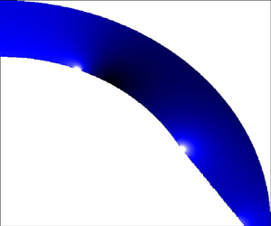
  $M$ in this case was 100. The resulting pressure and velocity fields are presented in figure 7 where the velocity shown is the absolute value determined through
 \begin{equation} v(\theta,r) = \sqrt{v_\theta(\theta,r)^2 + v_r(\theta,r)^2}.\end{equation}
Similar to the Cartesian flat plate case, the pressure distribution leads to large gradients between the permeable and impermeable boundaries at the internal plenum side. These then result in a strong concentration of velocity at these boundaries. In figure 8, the internal pressure and streamfunction distributions and the external outflow velocity are presented. The constant streamfunction at the internal boundary between the arc lengths of  $2.5$ and
  $5.5$ mm confirms the impermeable boundary, and the pressure distribution outside of this region also correctly replicates the required constant plenum pressures. Figure 8 also contains a numerical comparison, that relates to the result of a COMSOL simulation using a mesh of approximately
  $10\,000$ cells. A mesh independence study was carried out which showed that a finer mesh leads to a maximum difference of 0.2 % in the velocity field when the mesh size is doubled. This is deemed as an acceptable accuracy and the results discussed in the following relate to the coarser mesh. The agreement of the pressure and velocity values at the shown boundaries is excellent with the exception of slight oscillations at an arc length of
  $0$ mm due to the Gibbs phenomenon. In this case, the steep decrease of the outflow velocity away from the symmetry plane is mainly due to the rapidly increasing thickness of the porous domain. The rival effect of a lower pressure for greater
  $\theta$ cannot compete with the influence of a thinner wall. Naturally, the outflow velocity is lowest above the impermeable section, as this region redirects a majority of the fluid flow laterally, which would have otherwise contributed to the radial outflow. Toward the rear of the domain at arc lengths
  $>5$ mm, the outflow velocity increases again due to the much lower external pressure (see figure 6).

Figure 6. Sketch of cylindrical example (a) with pressure boundary conditions (b).

Figure 7. Pressure and velocity field in porous domain of wedge leading edge case.

Figure 8. Flow field along boundaries  $r=R_i(\theta )$, and
  $r=R_e$. (a) Pressure and streamfunction at internal boundary
  $r=R_i(\theta )$ and (b) velocity magnitude at external boundary
  $r=R_e$.
6. Conclusion
This work presents an analytical solution to steady state porous flows encountered in transpiration cooling applications. The steady state incompressible porous flow field is described through potential flow theory and a closed analytical solution is derived for Cartesian and cylindrical coordinates. The solution allows arbitrary wall thickness distributions, arbitrary pressure distributions and arbitrary amounts and locations of impermeable boundaries. General solutions for the pressure and velocity fields are presented and special solutions are provided for the external boundary outflow velocity. This allows a direct calculation of the expected mass injection distribution of a transpiration cooling architecture. This work allows fast and accurate calculations of flow fields in porous media which can be used as validation tools for numerical simulations or as a fast design tool for porous transpiration cooling architectures.
Acknowledgements
We would like to extend our gratitude to L. Vandeperre of Imperial College London, J. Merrifield of Fluid Gravity Engineering, L. di Mare and the entire Oxford Hypersonics group for the fruitful and interesting discussions.
Funding
The authors would like to greatly acknowledge the funding of this work by DARPA under the MACH program (reference HR001119S0022) and the Engineering and Physical Sciences Research Council (reference EP/P000878/1).
Declaration of interest
The authors report no conflict of interest.


