


1. Introduction
Total helicity,  $H$, is a measure of the topological complexity of a tangled vortical flow field. It is defined as the integral of helicity density,
  $h=\boldsymbol {u} \boldsymbol {\cdot } {\boldsymbol {\omega }}$, over the fluid domain surrounding the vortex field (see (7.1)). Total helicity is a conserved quantity in inviscid flows, as found in superfluids (Salman Reference Salman2017; Kedia et al. Reference Kedia, Kleckner, Scheeler and Irvine2018), however, it may increase or decrease in the presence of viscous effects. The latter are always dissipative in nature and are responsible for the annihilation of negative/positive helicity density, which results in a total helicity increase/decrease. The rate of change of total helicity,
  $\textrm {d}H/\textrm {d}t$, is proportional to the superhelicity,
  $\langle s \rangle \equiv \langle \boldsymbol {{\omega }}\boldsymbol {\cdot } (\boldsymbol {\nabla }\times \boldsymbol {{\omega }}) \rangle$ through the kinematic viscosity
  $\nu$ (see (7.2)).
The understanding of helicity dynamics is of crucial importance in a wide variety of fields, such as liquid crystals (Tkalec et al. Reference Tkalec, Ravnik, Čopar, Žumer and Muševič2011), optical (Dennis et al. Reference Dennis, King, Jack, O'Holleran and Padgett2010) and biological structures (Chichak et al. Reference Chichak, Cantrill, Pease, Chiu, Cave, Atwood and Stoddart2004; Han et al. Reference Han, Pal, Liu and Yan2010), and beyond.
In the case of viscous vortex flows, tangled vortex fields tend to evolve towards simpler topologies. Knot and link are two basic states of tangled vortex fields, which are explored in this manuscript; unknotting and unlinking are the respective processes responsible for their break down into a simpler topology, and hence change in total helicity. Recent experimental studies (Kleckner & Irvine Reference Kleckner and Irvine2013; Scheeler et al. Reference Scheeler, Kleckner, Proment, Kindlmann and Irvine2014) have revealed how the zeroing of total helicity during the unknotting of vortex rings does not happen abruptly. In fact, during the unknotting process, the measured helicity appeared to be ‘relatively’ unchanged. However, owing to the presence of a broad spectrum of small spatial and temporal scales inaccessible by the experiments, a clear demonstration as to whether helicity is conserved or not through such reconnection events has been deemed to be unclear by Moffatt (Reference Moffatt2017). Moreover, the reported experimental measurement of helicity by Irvine's group relied solely on centreline vorticity and velocity information, thus not strictly corresponding to the total helicity, which is a global integral quantity. Accurate direct numerical simulations (DNS) able to simultaneously capture the entirety of the topologically complex vortex field and the small-scale details of the viscous reconnection are thus warranted. This is only achievable by relying on adaptive mesh refinement (AMR) computational frameworks such as that developed by the current authors (Zhao & Scalo Reference Zhao and Scalo2020; Zhao et al. Reference Zhao, Yu, Chapelier and Scalo2021).
The current manuscript focuses on vortex fields undergoing unknotting and unlinking processes initiated by local viscous reconnection events. The latter have been studied extensively in the past decades. DNS of Navier–Stokes equations of a pair of anti-parallel vortex tubes has been the most commonly adopted set-up (Hussain & Duraisamy Reference Hussain and Duraisamy2011; Van Rees, Hussain & Koumoutsakos Reference Van Rees, Hussain and Koumoutsakos2012; Mcgavin & Pontin Reference Mcgavin and Pontin2018), with recent efforts simulating circulation-based Reynolds numbers up to  $Re_\varGamma =\varGamma /\nu =40\ 000$ (Yao & Hussain Reference Yao and Hussain2020). Van Rees et al. (Reference Van Rees, Hussain and Koumoutsakos2012) and McGavin & Pontin (Reference McGavin and Pontin2019) have also investigated anti-parallel reconnections of twisted vortex tubes, with twist helicity created by initial axial flow.
Although these studies provided insight into circulation transfer scaling and the vortex structure created in the reconnection events, they are based on minimal-flow-unit configurations – much simpler than the case of vortex knots/links – and do not directly address the question of total helicity conservation for topologically complex vortex flows.
In recent years, several numerical works have focused on topologically complex vortex flows (Kerr Reference Kerr2018; Xiong & Yang Reference Xiong and Yang2019). However, the computational restrictions inherently associated with uniform Cartesian grids limited these studies to a small simulation domain and thick vortex cores. Some other works have focused on the influence of topological properties on the dynamics of vortex torus knots in inviscid conditions (Ricca, Samuels & Barenghi Reference Ricca, Samuels and Barenghi1999; Oberti & Ricca Reference Oberti and Ricca2019).
Proper investigation of helicity dynamics requires a sufficiently large domain size to reduce the influence of boundary conditions while simultaneously guaranteeing DNS-level resolution of the small-scale vortical processes occurring in the reconnection region. This is particularly challenging for uniform-grid-based CFD methods like pseudo-spectral methods, which makes AMR the only feasible computational strategy to address helicity dynamics with high-fidelity numerical data.
In this work, DNS are performed with an AMR computational framework of two canonical vortex topologies, namely, a trefoil knot and two-ring link. For each case, four different initial core sizes are simulated, to investigate the influence of the core size on the helicity dynamics, and to assess whether there is any fundamental difference between thin-core and thick-core vortex dynamics and reconnections. The collision of two unlinked rings is also simulated to serve as an example of a topologically trivial simulation, i.e. exhibiting no total helicity change. For the sake of conciseness, the present analysis is focused on one circulation-based Reynolds numbers of  $Re_\varGamma =2000$. The key conclusion of this paper is that total helicity is not conserved through reconnection in topologically complex vortex problems, and that this occurs through a process of annihilation of the local helicity content connected to circulation transfer. This annihilation mechanism was first identified by Kimura & Moffatt (Reference Kimura and Moffatt2014) via their analysis to the local analytical solution of the Navier–Stokes equations associated with a pair of skewed Burger's vortex tubes. In this current work, the annihilation is examined with the DNS of the Navier–Stokes equations for the first time. Although this conclusion is independent of the Reynolds number, nonetheless, a comparison against data at
  $Re_\varGamma =6000$ is also carried out in the case of the trefoil vortex knot to show what high-Reynolds-numbers effects entail. The latter simply results in a larger variance of the instantaneous location of the reconnection sites and hence spatio-temporal inhomogeneities in the circulation transfer and superhelicity hotspots.
The paper is organized as follows: first, the governing equations and the design of the initial condition for each simulation case is presented in § 2; then, the simulation approach is briefly described in §§ 3, 4 and 5 and the simulation results are presented and discussed in § 6; finally, an analytical model explaining the mechanism responsible for the change in total helicity is provided in § 7, followed by the conclusions of this paper in § 8.
2. Governing equations
The flow motion considered is assumed to be governed by the set of compressible Navier–Stokes equations:
 \begin{equation} \frac{\partial{\boldsymbol{{w}}}}{\partial{t}}+\boldsymbol{{\nabla}}\boldsymbol{\cdot} [{\boldsymbol{\mathsf{F}}}_{{c}}(\boldsymbol{{w}})-{\boldsymbol{\mathsf{F}}}_{{v}}(\boldsymbol{{w}},\boldsymbol{\nabla} \boldsymbol{{w}})]=\boldsymbol{{0}}, \end{equation}
where  $\boldsymbol {{w}}=(\rho ,\rho \boldsymbol {{U}},\rho E)^{\textrm {T}}$ is the vector of conserved variables
  $\rho , \boldsymbol {{U}}$ and
  $E$, the density, velocity and total energy, respectively, and
  $(\boldsymbol {\nabla } \boldsymbol {{w}})_{ij} = \partial {w_i}/\partial {x_j}$ is its gradient. The convective and viscous flux tensors
  ${\boldsymbol{\mathsf{F}}}_{{c}},{\boldsymbol{\mathsf{F}}}_{{v}}\in \mathbb {R}^{5\times 3}$ read
 \begin{equation} {\boldsymbol{\mathsf{F}}}_{{c}}= \left( \begin{array}{@{}c@{}} \rho\boldsymbol{{U}}^{{T}}\\ \rho\boldsymbol{{U}}\otimes\boldsymbol{{U}}+ p{\boldsymbol{\mathsf{I}}}\\ (\rho E+p )\boldsymbol{{U}}^{{T}} \end{array}\right),\quad \mathrm{and}\quad {\boldsymbol{\mathsf{F}}}_{{v}}= \left( \begin{array}{@{}c@{}} \boldsymbol{{0}}\\ \boldsymbol{\tau}\\ \boldsymbol{\tau}\boldsymbol{\cdot} \boldsymbol{{U}}-\lambda\boldsymbol{{\nabla}} T^{{T}} \end{array}\right) , \end{equation}
where  $T$ is the temperature,
  $p$ is the pressure,
  $\lambda$ is the thermal conductivity of the fluid and
  ${\boldsymbol{\mathsf{I}}} \in \mathbb {R}^{3\times 3}$ is the identity matrix. For a Newtonian fluid, we have
 \begin{equation} \boldsymbol{\tau}=2\mu{\boldsymbol{\mathsf{S}}}, \end{equation}
where  $\mu$ is the dynamic viscosity and
 \begin{equation} {\boldsymbol{\mathsf{S}}}=\tfrac{1}{2}[\boldsymbol{\nabla} \boldsymbol{{U}}+\boldsymbol{\nabla} \boldsymbol{{U}}^{{T}}-\tfrac{2}{3}(\boldsymbol{{\nabla}}\boldsymbol{\cdot} \boldsymbol{{U}}){\boldsymbol{\mathsf{I}}}]. \end{equation}
The ideal gas law is considered for the closure of the system of equations, namely,
 \begin{equation} p=(\gamma-1)(\rho E-\tfrac{1}{2}\rho\boldsymbol{{U}}\boldsymbol{\cdot} \boldsymbol{{U}}), \end{equation}
where  $\gamma$ is the heat capacity ratio.
The solver is based on a staggered grid arrangement, which provides superior accuracy and robustness compared with a fully collocated approach (Lele Reference Lele1992). The time integration is performed using a third-order Runge–Kutta scheme.
For the presently considered computations, the speed of sound is arbitrarily selected as  $c_{{ref}}=5V_{{max}}$, where
  $V_{{max}}$ is the maximum velocity magnitude at the initial condition. The maximum Mach number is achieved during reconnection and it does not exceed 0.25 in all cases simulated. This choice yields near-incompressible flow dynamics. As a result, the compressibility effect is not the focus of the current work. The discussion of acoustic noises generation associated with vortex reconnections can be found in the paper by Daryan, Hussain & Hickey (Reference Daryan, Hussain and Hickey2020). Simulations are initialized with unitary density and temperature fields, equal to the reference values
  $\rho _{{ref}} = 1.0$ and
  $T_{{ref}}=1.0$. The gas constant is then defined by setting the reference pressure to
  $p_{{ref}}=\rho _{{ref}} c_{{ref}}^2/ \gamma$, where
  $\gamma =1.4$ is the ratio of specific heats. Levels of density, temperature and pressure are dimensionless and physically irrelevant, as the compressibility effects on the simulated hydrodynamics are negligible.
3. Computational set-up
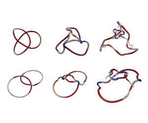
The initial conditions for a trefoil knot and a pair of linked rings is shown in figures 1(a and b), respectively. The initial symmetry of both set-ups yields multiple simultaneous and identical reconnections as both vortex structures propagate in the  $z$-direction. For each case, four different core sizes are simulated to assess their influence on the helicity dynamics during reconnection. The vortex filament of a trefoil knot is described via the parametric curve:
 \begin{equation} \boldsymbol{X}_{{knot}}(\theta) = \left( \begin{array}{@{}c@{}} R_{{min}}(\sin(\theta)+2\sin(2\theta)) \\ R_{{min}}(\cos(\theta)-2\cos(2\theta)) \\ R_{{min}}\sin(3\theta ) \end{array} \right), \end{equation}
where  $R_{{min}}$ is the minimum radius. The mean radius
  $\bar {R}=({1}/{4{\rm \pi} })\int _0^{2{\rm \pi} } |\textrm {d}\boldsymbol {X}_{{knot}}(\theta )/\textrm {d}\theta | \, \mathrm {d} \theta$ will be used as a characteristic length scale in the present study. We choose the knot half-thickness to be
  $R_{{min}}$, which results in
  $\bar {R}=2.294 R_{{min}}$. The parametric equation describing the two initially linked rings is given by
 \begin{equation} \boldsymbol{X}_{{link},\pm} (\theta) = \left(\begin{array}{@{}c@{}} \bar{R}\cos\theta \mp \eta \bar{R}, \\ \bar{R} \cos\alpha \sin\theta, \\ \pm \bar{R} \sin\alpha \sin\theta \end{array}\right), \end{equation}
where the subscripts  $\pm$ differentiate the two rings. Values of
  $\eta =0.7$ and
  $\alpha =10^\circ$ are chosen to yield a short time for unlinking. The parametric equations for the unlinked rings in the colliding-ring problem (figure 1c) are given by
 \begin{equation} \boldsymbol{X}_{{coll}, \pm} (\theta) = \left(\begin{array}{@{}c@{}} \bar{R}\cos\theta \\ -\bar{R} (\cos\alpha \sin\theta \pm \cos\alpha \pm \eta) \\ \mp \bar{R} \sin\alpha \sin\theta \end{array}\right), \end{equation}
where  $\eta =0.1$ and
  $\alpha =45^\circ$ are chosen. In this paper,
  $\bar {R}=33.75$ mm is used for all the three problems, so that the total initial vortex length
  $l_0= 4{\rm \pi} \bar {R}$ in all three problems are the same.

Figure 1. Configurations for (a) trefoil knot, (b) linked rings and (c) colliding rings.
The flow field is initialized with the Biot–Savart Law with a kernel function  $K_v$ (Vatistas, Kozel & Mih Reference Vatistas, Kozel and Mih1991; Hoydonck, Van Bakker & Van Tooren Reference Hoydonck, Van Bakker and Van Tooren2010):
 \begin{equation} \boldsymbol{u}(\boldsymbol{x})={-}\frac{\varGamma}{4{\rm \pi} }\int{K_v\frac{(\boldsymbol{x}-\boldsymbol{X}(\theta)) \times\boldsymbol{t}(\theta)}{|\boldsymbol{x}-\boldsymbol{X}(\theta)|^3}\, \textrm{d} \theta} \quad K_v=\frac{|\boldsymbol{x}-\boldsymbol{X}(\theta)|^3}{{(|\boldsymbol{x}- \boldsymbol{X}(\theta)|^{4}+{a}^{4})}^{{3}/{4}}}, \end{equation}
where  $\boldsymbol {t}(\theta )$ is the unit vector tangent following the parametric function
  $\boldsymbol {X}(\theta ), \varGamma$ is the circulation and
  $a$ is the Lamb–Oseen core size. With this kernel function, a Gaussian vorticity profile,
  $\omega (r) = \varGamma /{\rm \pi} a^2 \exp {( -r^2/a^2 )}$, which describes the Lamb–Oseen model, can be obtained, where
  $r$ is the radial distance from the centre of the vortex tube. Furthermore, the relation
  $\partial p /\partial r = \rho V^2/r$ is used to initialize the pressure field with the energy equation. In this paper, all the simulations are carried out with circulation of
  $\varGamma = 0.02$ m
 $^2$ s
 $^{-1}$ and fluid viscosity of
  $\nu = 10^{-5}$ m
 $^2$ s
 $^{-1}$. The circulation-based Reynolds number is
  $\mathrm {Re}_{\varGamma } = \varGamma /\nu = 2000$ for all the simulations in the current and the next section.
The effective area and radius of a vortex tube are defined as  $A_{{eff}} = {(\int {\omega \, \mathrm {d} A})^2}/{\int {\omega ^2 \, \mathrm {d} A}}$ and
  $r_c = \sqrt {{A_{{eff}}}/{{\rm \pi} }}$, respectively, where
  $\omega$ is the vorticity magnitude and
  $\mathrm {d} A$ is the differential area on a normal cross-section of the vortex tube. A Lamb–Oseen vortex core follows the relation
  $r_c^2 = 2a^2$. In this paper, the radii
  $r_c = 2$, 4, 6 and 8 mm (or
  $r_c/\bar {R}=0.059$, 0.119, 0.178, 0.237) are chosen for the trefoil knot case;
  $r_c = 2$, 3, 4 and 4.5 mm (or
  $r_c/\bar {R}=0.059$, 0.089, 0.119, 0.133) for the linked two-rings case; and
  $r_c = 2$ mm for the colliding pair of rings.
4. Adaptive mesh refinement
All simulations are carried out at DNS resolutions relying on the high-order compact finite-difference adaptive-mesh refinement Navier–Stokes code VAMPIRE (Zhao & Scalo Reference Zhao and Scalo2020). A vorticity-based sensor function is chosen as the refinement criterion and regions with negligible vorticity magnitude are coarsened to save computational resources.
For each simulation, before time advancement, a sensor estimating the discretization error of the sampled initial condition is ran on all the blocks to determine whether the mesh should be locally refined; such process is repeated until convergence of the AMR Octree structure. A sample of the resulting adaptively refined mesh at time  $t=0$, as well as subsequent times, is shown in the supplementary movies available at https://doi.org/10.1017/jfm.2021.455 for each simulated case (supplementary movie 1 for trefoil knot and supplementary movie 2 for two-ring link).
In this work, our goal is to apply the AMR code to fully resolve the vortex reconnection dynamics. Therefore, we choose to use a vorticity-based sensor, defined in the non-dimensional form:
 \begin{equation} {f_\omega } = \frac{{|\boldsymbol{\nabla} (\omega )| \varDelta_{{local}} }}{{max ( {{ \omega , \omega_{{ref}}}} )}}, \end{equation}
where  $\varDelta _{{local}}$ is the local grid spacing,
  $\omega$ is the magnitude of vorticity, i.e.
  $\omega := |\boldsymbol {{\omega }}|$. This expression is the normalized gradient of vorticity by a local indicator of the vorticity magnitude. From a numerics perspective to avoid division by zero, an extra term
  $\omega _{{ref}}$ is added to the denominator of the expression.
This reference vorticity value is expected to be a measure for the global level of vorticity magnitude. The sensor is expected to refine the grid in the region where the vortical features are significant, while coarsening the grid at the regions far away from the vortex ring, where the vorticity vanishes. More details of the numerics can be found in the paper by Zhao & Scalo (Reference Zhao and Scalo2020). The AMR structure is updated every time step. All of AMR simulation results presented in this paper are run at  $CFL=0.25$.
A large triply-periodic domain box with size  $L=0.44$ m is made possible by the AMR framework, which allows minimization of numerical artifacts on the helicity dynamics caused by the periodic boundary conditions. Figures 2(a) and 2(b) show the simulated vortex structure relative to the total computational domain size, and the AMR grid at a particular moment in the trefoil evolution, respectively.

Figure 2. AMR grid set-up for the trefoil simulation with  $r_c=2$ mm at
  $t\varGamma /\bar {R}^2 = 3.69$. Isosurfaces are for
  $Q\bar {R}^4/\varGamma ^2=323$, coloured by helicity density
  $h$. Panels (a) and (b) show the block set-up of the entire simulation domain.
5. Grid sensitivity analysis
To verify the grid independence of the results, a systematic grid refinement process is carried out until the two finest simulations have reached a negligible difference in enstrophy and total helicity levels.
The AMR grid set-up for the simulations for the trefoil knot and two-ring link with different initial core radius  $r_c$ are shown in table 1. The grid resolution can be represented by
  $L/\varDelta$, where
  $\varDelta$ is the finest grid size for an AMR grid. The grid resolution is increased for each case until a satisfactory grid convergence behaviour is observed. For most of the simulations, the 9-level 12-point AMR grid achieves a good overlapping with the second finest grid level. For the trefoil case with
  $r_c=8$ mm, it is found that the 8-level 12-point AMR grid is sufficient to reach a good grid convergence.
Table 1. Grid resolution and line style in figure 3 for different cases. Line styles represent different grid resolutions. Solid line represents the highest grid resolution available for that specific case. Here,  $d$ is the number of levels of the AMR grid,
  $N^3$ is the number of cell in each direction within each AMR block,
  $L$ is the domain size and
  $\varDelta$ is the minimum grid spacing.

For each simulation case, the grid sensitivity is monitored for two quantities of interest, which are enstrophy  $\varXi =\iiint {\tfrac {1}{2}\omega ^2\, \mathrm {d} V}$ and helicity
  $H=\iiint {\boldsymbol {{u}} \boldsymbol {\cdot } \boldsymbol {{\omega }} \, \mathrm {d} V}$. The grid convergence for these two quantities is shown in figure 3, with different grid resolution represented by the different line-styles listed in table 1.

Figure 3. Total enstrophy  $\varXi$ and total helicity
  $H$ for trefoil knot (panels (a,b) in blue) and two-ring link (panels (c,d) in purple) with different core sizes
  $r_c$. Vertical dashed bars are the time
  $t_1$ when circulation transfer is 50 % complete. Lines depicted as dotted, dashed and solid indicate progressive grid refinement (see table 1 for more details).
The finest calculations reach a box-size to minimum grid-spacing ratio of  $L/\varDelta =3072$ (or
  $\bar {R}/\varDelta =235.6$), where
  $\varDelta$ is the grid spacing of the leaf blocks. Only results from the finest calculations are included in this manuscript.
6. Simulation results
Figures 3 and 4 show the normalized total enstrophy  $\varXi =\iiint {\tfrac {1}{2}\omega ^2\, \mathrm {d} V}$ (proportional to the total kinetic energy viscous dissipation rate) and total helicity
  $H$ versus normalized time
  $t^* = t\varGamma /\bar {R}$. If the vortex tube has a Lamb–Oseen core structure, the initial volume-integrated enstrophy
  $\varXi$ can be estimated as
 \begin{equation} \varXi_0 = \left. \int_{\mathcal{V}}{\frac{1}{2}\omega^2\, \mathrm{d} \mathcal{V}} \right|_{t=0} \cong \frac{\varGamma^2 l_0}{2A_{{eff}}}, \end{equation}
which will be used to normalize the instantaneous value of  $\varXi$. Enstrophy tends to decrease at the beginning, because of the thickening of the vortex core owing to viscous dissipation. As reconnections start, two anti-parallel vortex tube segments approach each other and get squeezed, which leads to the local reduction of vortex core and enstrophy increase. After the completion of reconnection, the thickening of the vortex core and decrease of enstrophy resumes. Consistent with the Lamb–Oseen vortex tube model, a thinner vortex tube exhibits a faster enstrophy decay rate.

Figure 4. Total enstrophy (a) and total helicity (b) for colliding rings with  $r_c=2$ mm. In panel (b), total helicity for trefoil knot and linked rings is compared, plotted versus time normalized by the reconnection time
  $t_1$.
Circulation transfer is tracked during the reconnections with the vortex line method (see Appendix A for more details, also see figure 9c). The vertical dashed bars in figures 3 and 4 indicate the moment when the cumulatively transferred circulation  $\varGamma _t$ equals half of the initial one, i.e.
  $\varGamma _t = 0.5 \varGamma$. This moment is indicated as
  $t=t_1$ and it also corresponds, in all cases, to the peak in enstrophy. The
  $Q$-isosurface evolutions of the three vortex configurations outlined in figure 1 are shown in figure 5 all for
  $r_c=2$ mm.

Figure 5. Isosurfaces of  $Q\bar {R}^4/\varGamma ^2=323$ at different times coloured by helicity density for trefoil knot (a), two-ring link (b) and colliding rings (c) for
  $r_c=2$ mm.
The three chosen cases have different reconnection times owing to their different initial configurations. The reconnection time is also very sensitive to changes in the vortex core radius: a larger vortex core radius delays the reconnection time and prolongs the reconnection process itself. This is because the self-induced velocity of vortex tubes scales like  $\varGamma /4{\rm \pi} R_0 \ln (R_0/r_c)$, which in turn depends on the ratio between core radius
  $r_c$ and the local radius of curvature
  $R_0$.
It can be noticed from figure 3 that the helicity in all the cases experiences a rapid increase through reconnection, whose halfway mark coincides with  $t=t_1$ defined above, hence suggesting a relation between helicity change and circulation transfer. Furthermore, the change in helicity is sharper for thinner cores and gentler for thicker cores. Note that with thicker cores, the initial helicity drops slightly compared with the thin-core cases, which arises from the self-intersection effect (also reported by Xiong & Yang Reference Xiong and Yang2019). For the knotted vortex and the two-ring linked problem, the evolution of total helicity experiences two stages: a linear ramp-up stage occurring during the circulation transfer (see more details in the following section) and a relatively more gradual change in the absence of reconnections. However, this two-stage behaviour is not present in the colliding-ring case (see figure 4), where the total helicity remains unchanged. While the latter result is trivially expected, it serves as a sanity check showing that the presence of a helicity change is not a numerical artefact but rather indeed a result of a physical process that is analytically described in the next section.
7. Dynamics of helicity through reconnections
7.1. Annihilation of negative helicity density hotspots at the reconnection sites
This section discusses the mechanisms behind the total helicity change occurring during the unlinking/unknotting processes. The analysis will focus only on the trefoil knot results for  $r_c=2$ mm simply for the sake of conciseness and without loss of generality, because the same interpretation is applicable to other complex vortex configurations and for different core radii. The total helicity is the integral of helicity density over the entire fluid domain:
 \begin{equation} H = \iiint h \, \textrm{d} \mathcal{V}. \end{equation}
In incompressible viscous flows, total helicity is governed by the equation (Moffatt Reference Moffatt1969):
 \begin{equation} \frac{\mathrm{d} H}{\mathrm{d} t} = \iiint{ - 2\nu \boldsymbol{{\omega}} \boldsymbol{\cdot} ( \boldsymbol{\nabla} \times \boldsymbol{{\omega}} ) \, \mathrm{d} \mathcal{V}} ,\end{equation}
whose right-hand side contains the product of viscosity and superhelicity  $s = \boldsymbol {{\omega }} \boldsymbol {\cdot } ( \boldsymbol {\nabla } \times \boldsymbol {{\omega }} )$, which is the source of the helicity change analysed in the previous sections.
Figure 6(a) shows isosurfaces of negative superhelicity  $-s$ during reconnection, which display the shape of two pairs of almost identical petals. The petal pair structure is determined by the particular vortex centreline geometry near the tipping points, a term introduced by Moffatt & Kimura (Reference Moffatt and Kimura2019a) for the first time, which refer to the points of closest approach of the vortices of the reconnection region. As shown in figure 7(a,b), a local coordinate system centred at the middle of the threads is set-up, with
  $\tilde {y}$–
 $\tilde {z}$ defining the dividing plane, and the
  $\tilde {x}$-axis aligning the direction of bridge formation. Figure 7(b) prominently shows that two vortex tubes that are about to reconnect become nearly anti-parallel owing to the self-induced motion. This choice of local coordinate system facilitates the analysis of this local nearly anti-parallel reconnection problem, where previous knowledge obtained from the extensively studied anti-parallel reconnection problems can be applied. The flattening of curvature at tipping points in viscous reconnection has been reported by multiple numerical studies (Yao & Hussain Reference Yao and Hussain2020; Zhao et al. Reference Zhao, Yu, Chapelier and Scalo2021). The radii of curvature reach a minimum value and then increase as the two vortex tubes approach each other. This arises from the jet flow induced by two newly formed bridges pushing two threads away from each other. As reconnection occurs, the steep gradient of vorticity magnitude
  $\omega$ is aligned in the direction of
  $\tilde {x}$ (as shown by the purple arrow in figure 7b), and the direction of
  $\boldsymbol {\nabla } \times \boldsymbol {{\omega }}$ is along the
  $\tilde {z}$ direction (as shown by the purple arrow in figure 7a). The
  $\tilde {z}$-component of the vorticity vector is given by the geometry of the centrelines of the vortex tubes near the tipping points, and four ‘petals’ are formed in the four quadrants in the
  $\tilde {x}$–
 $\tilde {y}$ plane, respectively. The red petals (positive superhelicity) are formed in the quadrants where
  $\boldsymbol {{\omega }}_{\tilde {z}}$ aligns with
  $\boldsymbol {\nabla } \times \boldsymbol {{\omega }}$, whereas the blue petals (negative superhelicity) are formed in the quadrants where
  $\boldsymbol {{\omega }}_{\tilde {z}}$ and
  $\boldsymbol {\nabla } \times \boldsymbol {{\omega }}$ are pointing in opposite directions.

Figure 6. Iso-surface of vorticity magnitude  $\omega = 34.17\varGamma /\bar {R}^2$ for the trefoil knot shown as transparent grey: (a) coloured isosurfaces of superhelicity
  $-s\bar {R}^5/\varGamma ^2=\pm 8210$; (b) coloured isosurfaces of helicity density
  $h\bar {R}^3/\varGamma ^2=\pm 9.6$. Red and blue are for positive and negative values, respectively.

Figure 7. Centreline of the trefoil knot shown in blue extracted from DNS at  $t\varGamma /\bar {R}^2=2.792$ and
  $r_c=2$ mm, viewed from two different viewing angles. The green dashed box shows the local coordinate located at the centre of the reconnection site. Blue and red shaded regions are qualitative depictions of positive and negative superhelicity spots, respectively. The resolved structure from the simulation is shown in figure 6.
However, small differences caused by the asymmetric twist/axial-flow distribution manifest themselves only in a slight shift of the larger, more coherent scales (i.e. the petals). As a result, this petal form has a nearly symmetric pattern, with the positive and negative sides of the dipole almost cancelling each other (and hence almost yielding a zero net total helicity change). However, such non-zero net difference is ultimately responsible for the rate of change of the total helicity and is better illustrated by visualizing volumetrically filtered data (figure 8). In this work, the centreline of a vortex tube is defined as the line connecting the critical points, where vorticity and velocity vectors are aligned.

Figure 8. Plots based on locally averaged solution of the trefoil knot with  $r_c = 2$ mm, where the value on each point is the average of 16
 $^3$ nearby grid points from the DNS solution. Panels (a,b,d,e): contour plots of
  $-S_z$ and
  $H_z$ at (a,b)
  $t\varGamma /\bar {R}^2=2.95$ and (d,e)
  $t\varGamma /\bar {R}^2=3.476$. Here,
  $H_z$ is defined as
  $H_z = \int _{-\infty }^{\infty } {h \, \mathrm {d} z}$ and
  $S_z$ is defined as
  $S_z = \int _{-\infty }^{\infty } {s \, \mathrm {d} z}$. Panels (c) and (f): isosurfaces of superhelicity
  $-s\bar {R}^5/\varGamma ^2=2730$ (red) and
  $-2730$ (blue), with the transparent vortex tube as
  $\omega = 11.39\varGamma /\bar {R}^2$.
Figure 8(a) shows that superhelicity hotspots are concentrated in the reconnection sites during unknotting, while figure 8(b) shows negative helicity hotspots in the same regions, which suggest an annihilation mechanism of negative helicity by the negative superhelicity hotspots and hence a total helicity rise. After the completion of the unknotting, the superhelicity hotspots disappear (figure 8d), as well as the negative helicity spots at the reconnection sites (figure 8e), while the rest of the helicity distribution remains almost unchanged. The negative net helicity content at the reconnection sites forming on the brink of reconnection (figure 6b) arise from an asymmetry in the anti-parallel vortex tubes structure before reconnection, which leads to differences in the induced axial flow and hence helicity. During the reconnection, any net non-zero helicity content at the reconnection sites is rapidly annihilated via a viscous circulation transfer mechanism (discussed below). This annihilation mechanism was first identified by Kimura & Moffatt (Reference Kimura and Moffatt2014) in their analysis of a pair of skewed Burger's vortex tubes. In the cases of the trefoil knot and the pair of linked rings, the net helicity content at the reconnection sites being dissipated is negative, therefore leading to a helicity rise.
7.2. Relation between circulation transfer and helicity annihilation
In this section, we provide the analytical relation between circulation transfer and the helicity annihilation rate.
Figure 9 shows the temporal progression of the circulation transfer along with the helicity ramp for both the trefoil knot and two-ring link problem with  $r_c=2$ mm, which shows a clear synchronization between these two processes. The method of calculating transferred circulation is described in Appendix A. The slight delay in the total helicity change is attributed to a decrease in helicity occurring in the rest of the vortex loop, away from the reconnection sites. An attempt is made in figure 9(c,d) to estimate the magnitude of the helicity rise with the integral of the helicity density limited to a box enclosing the reconnection site, denoted as
  ${\rm \Delta} H$, at the moment
  $\varGamma _t/\varGamma \approx 5\,\%$. The box has its centre located in the middle of two tipping points on the vortex centreline, and covers the span of the anti-parallel tubes from the tipping point to the location with a separation distance of
  $2D_{{tip}}$. Here,
  $D_{{tip}}$ is the separation distance between two tipping points at this moment. Figure 9(a,b) shows that this method gives an acceptably accurate estimate of the helicity change, which suggests that the latter arises from hydrodynamic processes confined at the reconnection sites.

Figure 9. The circulation transfer (blue) of trefoil knot (a) and two-ring link (b) for  $r_c = 2$ mm compared with the time series of helicity change (red), with dashed lines marking
  ${\rm \Delta} H$ multiplied by the number of reconnection sites; (c) circulation transfer tracked by vortex lines for trefoil at
  $t^*=2.792$; (d) visualization of a box centred between two tipping points to evaluate
  ${\rm \Delta} H$ at
  $t^*=2.634$.
This consideration inspires the following analytical derivation to establish the relationship between circulation transfer and the helicity annihilation. First, the circulation transfer rate for a pair of anti-parallel vortices can be derived following the approach used by Mcgavin & Pontin (Reference Mcgavin and Pontin2018). With the simplified configuration of an anti-parallel reconnection qualitatively shown in figure 10, the circulation can be written as the vorticity flux passing through the plane  $A$, whose boundary is the yellow–green loop. The yellow edge is a straight line passing through the null point and perpendicular to the anti-parallel threads (along the
  $z$-direction). The change rate of the circulation passing, can be evaluated using Stokes’ theorem:
 \begin{align} \dot{\varGamma} \equiv \frac{\mathrm{d} \varGamma}{\mathrm{d} t} & = \frac{\partial}{\partial t} \int_A { \boldsymbol{{\omega}}\boldsymbol{\cdot} \boldsymbol{{n}} \, \mathrm{d} A} \nonumber\\ & = \int_A { \frac{\partial \omega}{\partial t} \boldsymbol{\cdot} \boldsymbol{{n}} \, \mathrm{d} A} \nonumber\\ & = \int_A { [ \boldsymbol{\nabla} \times (\boldsymbol{{v}}\times \boldsymbol{{\omega}}) - \nu \boldsymbol{\nabla} \times (\boldsymbol{\nabla} \times \omega) ] \boldsymbol{\cdot} \boldsymbol{{n}} \, \mathrm{d} A} \nonumber\\ & ={-}\nu \oint_{\delta A} { ( \boldsymbol{\nabla} \times \boldsymbol{{\omega}} ) \boldsymbol{\cdot} \mathrm{d} \boldsymbol{{l}}}, \end{align}
where the integral along green lines is zero, because  $\boldsymbol {\nabla } \times \boldsymbol {{\omega }}$ vanishes. A similar analysis was used by Moffatt & Kimura (Reference Moffatt and Kimura2019b) to analyse the build-up of the maximum vorticity in a reconnection event with an analytical method.

Figure 10. Qualitative plot of selected vortex lines during the interaction of anti-parallel vortex tubes (red, threads; blue, reconnected bridges). The arrows form a loop enclosing a plane through which one of the vortex tubes pass.
Next, we consider a minimized 4-element reconnection setting surrounding a null-point, as shown in figure 11(a,b). The four elements are placed in a 2-by-2-by-1 array, with the null-point in the middle, two layers in the  $x$- and
  $y$-directions, and a single layer in the
  $z$-direction. Each element has an edge length of
  $\delta$, which is a characteristic finite length scale defining the size of the reconnection site. This analysis is to establish the relationship between circulation transfer and the helicity annihilation, carried out on a two-dimensional anti-parallel reconnection problem between two infinitesimal vortex filaments of the same circulation
  $\textrm {d}\varGamma$ but with different axial flow velocities and hence helicity (figure 11).

Figure 11. (a,b) Kinematics of a reconnection of infinitesimal vortex filaments with a discretization by cells with an edge length of  $\delta$; (c,d) the reconnection site viewed from a different angle, with the Stokes surface highlighted.
We take the two parallel vortex filaments as initially oriented along the  $y$-axis, and the coordinate system used for this derivation as located at the mid-point between the two filaments, about which the reconnection happens. The circulation is transferred from the
  $y$-direction to the
  $x$-direction. The two reconnecting anti-parallel vortex filaments carry an infinitesimal circulation
  $\mathrm {d} \varGamma$, and have axial flow velocities
  $\bar {u}_1$ and
  $\bar {u}_2$. After time
  $\mathrm {d} t$, these two vortex filaments are reconnected and circulation is transferred into the
  $x$-direction, with the local
  $x$-components of velocity
  $\bar {u}_3$ and
  $\bar {u}_4$. The vortex lines in the
  $x$–
$x$– $y$ plane do not pass though the null point (
 $\omega _x=\omega _y=0$), but a vortex line in the
  $z$-direction with magnitude
  $\omega _z$ passes through it. Here,
  $\bar {u}_1, \bar {u}_2, \bar {u}_3$ and
  $\bar {u}_4$ are mean axial velocities for the threads and bridges, and they are located at the face centres between two adjacent elements, as depicted in figure 11(c,d). This infinitesimal reconnection event and associated circulation transfer
  $\textrm{d}\varGamma$, entails infinitesimal changes in the quantities of
  $\bar {u}_1 + \mathrm {d} \bar {u}_1, \bar {u}_2 + \mathrm {d} \bar {u}_2, \bar {u}_3 + \mathrm {d} \bar {u}_3, \bar {u}_4 + \mathrm {d} \bar {u}_4$ and
  $\omega _z + \mathrm {d} \omega _z$.
The reconnection region is further discretized into cells, whose edge length  $\delta$ is a length scale for the width and the length of the reconnected filament segments (figure 11c,d). The infinitesimal helicity change in the control volume
  $2\delta \times 2\delta \times \delta$ through this reconnection is
 \begin{equation} \mathrm{d} H = H(t + \mathrm{d} t) - H(t). \end{equation}
To the first order of accuracy, the vorticity magnitude at the centre of each cell is  $\mathrm {d} \varGamma /\delta ^2$, thus
 \begin{align} H(t + \mathrm{d} t) &= \iiint_\varOmega { \boldsymbol{{\omega}}(t + \mathrm{d} t) \boldsymbol{\cdot} \boldsymbol{{u}}(t+ \mathrm{d} t)\, \mathrm{d} V} \nonumber\\ &= 2\delta^2(\bar{u}_3 + \mathrm{d} \bar{u}_3) (\mathrm{d} \varGamma/\delta^2) + 2\delta^2(\bar{u}_4 + \mathrm{d} \bar{u}_4)(-\mathrm{d} \varGamma/\delta^2), \end{align}
and
 \begin{align} H(t) &= \iiint_\varOmega { \boldsymbol{{\omega}}(t) \boldsymbol{\cdot} \boldsymbol{{u}}(t)\, \mathrm{d} V} \nonumber\\ &= 2\delta^2 \bar{u}_1 (\mathrm{d} \varGamma/\delta^2) + 2\delta^2 \bar{u}_2(-\mathrm{d} \varGamma/\delta^2). \end{align}
Hence,
 \begin{equation} \mathrm{d} H = 2\delta (\bar{u}_3 + \mathrm{d} \bar{u}_3 - \bar{u}_4 - \mathrm{d} \bar{u}_4) \,\mathrm{d} \varGamma - 2\delta (\bar{u}_1 - \bar{u}_2) \, \mathrm{d} \varGamma. \end{equation}
Note that  $\bar {u}_3$ and
  $\bar {u}_4$ do not contribute to the helicity of the filament before reconnection. Dropping the second-order terms in (7.7) yields
 \begin{equation} \mathrm{d} H = 2\delta^2 \omega_{z}\, \mathrm{d} \varGamma, \end{equation}
where
 \begin{equation} \omega_z = (-\bar{u}_1 + \bar{u}_2 + \bar{u}_3 - \bar{u}_4)/\delta. \end{equation}
In Appendix C, Taylor series expansion is performed at the null point, and shows that (7.8) gives the first-order approximation of the helicity change local to the null point.
For a local reconnection that happens only in a span of  $\delta z$ in the
  $z$-direction, the the circulation transfer rate (7.3) can be re-written as
 \begin{equation} \dot{\varGamma} ={-} \nu (\boldsymbol{\nabla} \times \boldsymbol{{\omega}})\boldsymbol{\cdot} \boldsymbol{{\delta}}_z, \end{equation}
where  $\boldsymbol {{\delta }}_z$ is a vector in the
  $z$-direction with a magnitude of
  $\delta$, which passes though the origin (figure 11c,d). Substituting equation (7.10) into (7.8), yields
 \begin{equation} \frac{\mathrm{d} H}{\mathrm{d} t} ={-} 2\nu \delta^3 \boldsymbol{{\omega}}\boldsymbol{\cdot} (\boldsymbol{\nabla} \times \boldsymbol{{\omega}}), \end{equation}
which recovers (7.2) at the reconnection spot.
In the current scenario of reconnection of anti-parallel vortex filaments,  $\bar {u}_3$ and
  $\bar {u}_4$ are radial components of velocity, and under Burger's vortex model, they are independent of
  $y$ and can be assumed to be
  $\bar {u}_3 \approx \bar {u}_4$. With this assumption, the substitution of (7.9) into (7.8) leads to
 \begin{equation} \frac{\mathrm{d} H}{\mathrm{d} t} ={-} \frac{\mathrm{d} \varGamma}{\mathrm{d} t} \frac{ \mathrm{d} H_1 + \mathrm{d} H_2 }{\mathrm{d} \varGamma} ={-} 2\delta ( \bar{u}_1 - \bar{u}_2) \dot{\varGamma}, \end{equation}
where  $\mathrm {d} H_1=2\delta \bar {u}_1\,\textrm {d}\varGamma$ and
  $\mathrm {d} H_2=-2\delta \bar {u}_2\,\textrm {d}\varGamma$ are the helicity content stored in the reconnected segments of the two vortex tubes. This expression indicates that the local helicity change rate at the reconnection spot can be written as the product of the local circulation transfer rate and the local helicity content carried by the reconnected segments of the vortex tube. This idea is further supported by the superhelicity isosurfaces based on the locally averaged solution (figure 8c,f), which shows that the superhelicity hotspots are exactly located at the bridging spots, where the circulation transfer occurs. In (7.12), a length scale
  $\delta$ appears, which stands for the length of the anti-parallel segments dissipated through reconnection. Its value is problem-specific, and depends on factors including strain rate, Reynolds number, vortex core thickness and so forth. As marked in figure 9(d), the blue box enclosing the reconnection site should have a length of the order of
  $2\delta$.
Note this explanation does not account for the turbulent cascade reconnections at higher Reynolds numbers, with successive secondary reconnections and spurious small-scale vortex bursting, which will add more complexity to the helicity annihilation process. Figure 12 in fact shows that the synchronization process between the circulation transfer and the helicity ramp is disturbed by fluctuations for the trefoil case with  $r_c=2$ mm at the higher Reynolds number
  $Re_\varGamma =6000$. Nevertheless, as shown by the results in this paper, the suggested model provides a robust explanation for global dynamics of helicity change through the unknotting/unlinking events. All of the lower
  $Re_{\varGamma }$ cases show an undisturbed synchronization between circulation transfer and helicity jump.

Figure 12. Comparison of the progression of the circulation transfer (blue) and its helicity change (red) of trefoil knot with  $r_c = 2$ mm at
  $Re_\varGamma =2000$ (—–) and
  $Re_\varGamma =6000$ (– – –). Here,
  $t_1$ is the time where
  $\varGamma _t/\varGamma =0.5$ for each case.
With the helicity annihilation mechanism being discussed above, it is interesting to consider the topological interpretation of the helicity annihilated through the reconnection event. It has been widely recognized that the total helicity for a vorticity field consists of writhe and twist; however, both writhe and twist are geometrical quantities defined for a global physical domain (Moffatt & Ricca Reference Moffatt and Ricca1992). Therefore, it is hard to rigorously judge to which form the locally dissipated helicity content belongs during reconnection. However, the geometric interpretation of the vorticity and velocity configuration shown in figure 11 may suggest that the dissipated helicity is in the twist form, because under the assumed anti-parallel configuration, the writhe helicity at the reconnection spot is almost zero. This is because when the vortex tube in an anti-parallel reconnection event is straight (or with zero curvature), then the axial velocity induced by local curvature of the vortex tube vanishes; therefore, the remaining part is given by the axial velocity induced by the far-field vorticity, which is a minor component. This interpretation aligns with the claim by Laing, Ricca & De Witt (Reference Laing, Ricca and De Witt2015). Therefore, the mechanism discussed in this work suggests a local annihilation mechanism of twist helicity in a viscous reconnection event.
8. Conclusion
With the support of DNS of the unknotting/unlinking of topological vortex flows, we have shown how total helicity is not conserved during the unknotting/unlinking process. A linearized analytical reconnection model has been derived quantitatively linking the the total helicity annihilation rate to viscous circulation transfer processes, hence confirming the fundamental mechanism responsible for the violation of helicity conservation.
Supplementary movies
Supplementary movies are available at https://doi.org/10.1017/jfm.2021.455.
Acknowledgements
The authors also want to thank the anonymous referees for their professional comments, which have greatly improved the quality of this paper.
Declaration of interests
The authors report no conflict of interest.
Funding
This work was supported by the Army Research Office's ARO-YIP Award (W911NF-18-1-0045) and inspired by the conversations with Dr M. Munson (Army Research Office Fluid Dynamics Program) and Prof. William Irvine (University of Chicago). The authors also acknowledge the support of the Rosen Center for Advanced Computing (RCAC) at Purdue, and the US Air Force Research Laboratory (AFRL) DoD Supercomputing Resource Center (DSRC) allocation under the subprojects ARONC00723015, ARONC38762387 and ARLAP02642530.
Appendix A. Circulation transfer calculation via vortex line tracking
In this work, the circulation transfer is tracked by the vortex line tracking method, as shown in figure 13. A cut-plane is made at a point with a distance from the reconnection spot and normal to the local vortex centreline. On this plane, a number of seed points are made with a honey-cell configuration, so that the seed points are uniformly distributed. The magnitude of the vorticity vector normal to the cut-plane  $\omega _n$ is taken as the strength of the vortex filament. Thus, the circulation of a specific vortex filament is written as
  $\varGamma _i = \omega _n\boldsymbol {\cdot } A_i$, where
  $A_i$ is the hexagon area. Only the vortex filaments with strength
  $\omega _n$ greater than 5 % of the maximum vorticity magnitude on the cut-plane are tracked (shown by red circles in figure 13a). The transferred circulation at a time step
  $\varGamma _t$ is calculated by summing up all the circulations of reconnected filaments, and the circulation transfer ratio is taken as
  $\varGamma _t/\varGamma$. Reconnected filaments can be easily identified by checking the orientation of each filament after passing the reconnection site.

Figure 13. The cut-plane selected to measure the circulation transfer rate, and the seed points sampled on the cut-plane with honeycomb configuration (black crosses). Only the seed points with more than 5 % of the maximum vorticity on the cut-plane are selected. Selected simulation is the trefoil knot with  $r_c=2$ mm at
  $t\varGamma /\bar {R}^2=2.792$, and the vortex tube is visualized by the vorticity isosurface
  $\omega \bar {R}^2/\varGamma =5.7$.
Appendix B. Sensitivity to box size
In Appendix A of the paper by Zhao et al. (Reference Zhao, Yu, Chapelier and Scalo2021), a sensitivity study on the box-size analysis is conducted, based on the trefoil-knot simulation, via a rigid two-point correlation analysis. It has been shown that a box size of  $6.67\bar {R}$ can sufficiently minimize the artefacts from the boundary conditions. In the present paper, we used an even larger box size of
  $13\bar {R}$. With AMR, an increase of box size does not significantly affect the computational cost, as it would if a standard Cartesian grid was employed.
Whereas the sensitivity study on the box size in Appendix A of the paper by Zhao et al. (Reference Zhao, Yu, Chapelier and Scalo2021) is performed based on kinetic energy and enstrophy, we here provide a new test for the sensitivity of the box size on the helicity result. As shown in figure 14, we used three different box sizes,  $L=6.5\bar {R}, L=13\bar {R}$ and
  $L=26\bar {R}$, to simulate the trefoil-knot case with
  $r_c=2$ mm, with the medium size
  $L=13\bar {R}$ being reported in the manuscript. This is achieved by using
  $N^3=18^3$ grid points in each block, and varying the levels to be
  $L=7$, 8, 9, for the small, medium and large cases, respectively. The comparison shows that as the domain size is sufficiently large (
 $L=6.5\bar {R}$), the helicity result is independent on the box size. Especially when the box size is changed from
  $L=13\bar {R}$ to
  $L=26\bar {R}$, the helicity curve
  $H$ is almost unchanged. This again confirms the conclusion drawn in Appendix A of the paper by Zhao et al. (Reference Zhao, Yu, Chapelier and Scalo2021), but from the helicity point of view.

Figure 14. Box-size sensitivity check on the trefoil knot case with  $r_c=2$ mm. (a) Domain-integrated enstrophy
  $\varXi$; (b) total helicity
  $H$.
$H$.
Appendix C. Derivation of the relation between circulation transfer rate and helicity change rate using Taylor series expansion
The arrangement under discussion is shown in figure 15, where the circulation transfer occurs in the  $x$–
$x$– $y$ plane around a null point
  $p0$. The vorticity vector at the null point is written to be
 \begin{equation} \boldsymbol{{\omega}}_0 =\begin{bmatrix} 0 \\ 0 \\ \omega_z \end{bmatrix}, \end{equation}
as at null point  $\omega _x = \omega _y = 0$. Here for simplicity, we denote its gradient to be
  $\boldsymbol {A}:=\boldsymbol {\nabla } \omega _0$, and its components in the
  $x$–
$x$– $y$ plane are
 \begin{equation} A_{11} := \frac{\partial \omega_x}{\partial x} \quad A_{12} := \frac{\partial \omega_x}{\partial y} \quad A_{21} := \frac{\partial \omega_y}{\partial x} \quad A_{22} := \frac{\partial \omega_y}{\partial y}. \end{equation}
At a particular time  $t$, the circulation transfer is driven by the change of vorticity gradient at the null point
  $p0$. Following the circulation conservation, we have
 \begin{equation} \frac{\mathrm{d} A_{21}}{\mathrm{d} t} ={-} \frac{\mathrm{d} A_{12}}{\mathrm{d} t} = C. \end{equation}
The change rate is denoted as  $C$. At time
  $t$, the vorticity vectors at
  $\omega _1$ to
  $\omega _4$ at the cell centre of the four elements can be expressed by the Taylor series expansion at null Point 0 as
 \begin{gather} \omega_{1,x}(t) ={-}\tfrac{1}{2}A_{11}\delta - \tfrac{1}{2}A_{12}\delta + O(\delta^2), \end{gather}
 \begin{gather}\omega_{1,y}(t) ={-}\tfrac{1}{2}A_{21}\delta - \tfrac{1}{2}A_{22}\delta + O(\delta^2), \end{gather}
 \begin{gather}\omega_{2,x}(t) ={-}\tfrac{1}{2}A_{11}\delta + \tfrac{1}{2}A_{12}\delta + O(\delta^2), \end{gather}
 \begin{gather}\omega_{2,y}(t) ={-}\tfrac{1}{2}A_{21}\delta + \tfrac{1}{2}A_{22}\delta + O(\delta^2), \end{gather}
 \begin{gather}\omega_{3,x}(t) = \tfrac{1}{2}A_{11}\delta - \tfrac{1}{2}A_{12}\delta + O(\delta^2) , \end{gather}
 \begin{gather}\omega_{3,y}(t) = \tfrac{1}{2}A_{21}\delta - \tfrac{1}{2}A_{22}\delta + O(\delta^2) , \end{gather}
 \begin{gather}\omega_{4,x}(t) = \tfrac{1}{2}A_{11}\delta + \tfrac{1}{2}A_{12}\delta + O(\delta^2) , \end{gather}
 \begin{gather}\omega_{4,y}(t) = \tfrac{1}{2}A_{21}\delta + \tfrac{1}{2}A_{22}\delta + O(\delta^2). \end{gather}
Following Helmholtz's first theorem:
 \begin{equation} \omega_{1,y} = \omega_{2,y}, \quad \omega_{3,y} = \omega_{4,y}, \quad \omega_{1,x} = \omega_{3,x}, \quad \omega_{2,x} = \omega_{4,x}, \end{equation}
yields
 \begin{equation} A_{11} = A_{22} = 0. \end{equation}
Therefore, the vorticity vectors are simplified as
 \begin{gather} \omega_{1,x}(t) ={-} \tfrac{1}{2}A_{12}\delta + O(\delta^2), \end{gather}
 \begin{gather}\omega_{1,y}(t) ={-}\tfrac{1}{2}A_{21}\delta + O(\delta^2), \end{gather}
 \begin{gather}\omega_{2,x}(t) = \tfrac{1}{2}A_{12}\delta + O(\delta^2), \end{gather}
 \begin{gather}\omega_{2,y}(t) ={-}\tfrac{1}{2}A_{21}\delta + O(\delta^2), \end{gather}
 \begin{gather}\omega_{3,x}(t) ={-}\tfrac{1}{2}A_{12}\delta + O(\delta^2), \end{gather}
 \begin{gather}\omega_{3,y}(t) = \tfrac{1}{2}A_{21}\delta + O(\delta^2) , \end{gather}
 \begin{gather}\omega_{4,x}(t) = \tfrac{1}{2}A_{12}\delta + O(\delta^2) , \end{gather}
 \begin{gather}\omega_{4,y}(t) = \tfrac{1}{2}A_{21}\delta + O(\delta^2). \end{gather}
The circulation at time  $t$ is written as
 \begin{gather} \varGamma_y(t) ={-}\tfrac{1}{2}A_{21}\delta^3 + O(\delta^4), \end{gather}
 \begin{gather} \varGamma_x(t) ={-}\tfrac{1}{2}A_{12}\delta^3 + O(\delta^4). \end{gather}
The velocity at null point is written as
 \begin{equation} \boldsymbol{{u}}_0 =\begin{bmatrix} u_{0,x} \\ u_{0,y} \\ u_{0,z} \end{bmatrix}, \end{equation}
and the components of the velocity gradient tensor in the  $x$–
$x$– $y$ plane are denoted as
 \begin{equation} B_{11} := \frac{\partial u_x}{\partial x} \quad B_{12} := \frac{\partial u_x}{\partial y} \quad B_{21} := \frac{\partial u_y}{\partial x} \quad B_{22} := \frac{\partial u_y}{\partial y}. \end{equation}
Figure 15. The four-element configuration around the null point used for a Taylor series expansion analysis used in Appendix C. (a) Vorticity components; (b) velocity components.
Assume that the two-dimensional reconnection happens only in the  $x$–
$x$– $y$ plane, with symmetry with respect to the
  $z$-direction: i.e.
 \begin{equation} \frac{\partial}{\partial z} ({\cdot}) = 0. \end{equation}
Then, the continuity equation at the null point gives
 \begin{equation} B_{11} + B_{22} = 0, \end{equation}
and the definition of  $\omega _z$ can be expressed as
 \begin{equation} \omega_z = \frac{\partial u_y}{\partial x} - \frac{\partial u_x}{\partial y} = B_{21} - B_{12}. \end{equation}
Then we can denote the change rate of velocity component as
 \begin{gather} \frac{\partial B_{11}}{\partial t} ={-}\frac{\partial B_{22}}{\partial t} = D_1, \end{gather}
 \begin{gather}\frac{\partial B_{12}}{\partial t} = D2, \quad \frac{\partial B_{21}}{\partial t} = D_3, \end{gather}
and we can write the velocity components at the cell centres of the four elements as
 \begin{gather} u_{1,x}(t) = u_{0, x} - \tfrac{1}{2}B_{11}\delta - \tfrac{1}{2}B_{12}\delta + O(\delta^2), \end{gather}
 \begin{gather}u_{1,y}(t) = u_{0, y} - \tfrac{1}{2}B_{21}\delta - \tfrac{1}{2}B_{22}\delta + O(\delta^2) , \end{gather}
 \begin{gather}u_{2,x}(t) = u_{0, x} - \tfrac{1}{2}B_{11}\delta + \tfrac{1}{2}B_{12}\delta + O(\delta^2) , \end{gather}
 \begin{gather}u_{2,y}(t) = u_{0, y} - \tfrac{1}{2}B_{21}\delta + \tfrac{1}{2}B_{22}\delta + O(\delta^2) , \end{gather}
 \begin{gather}u_{3,x}(t) = u_{0, x} + \tfrac{1}{2}B_{11}\delta - \tfrac{1}{2}B_{12}\delta + O(\delta^2) , \end{gather}
 \begin{gather}u_{3,y}(t) = u_{0, y} + \tfrac{1}{2}B_{21}\delta - \tfrac{1}{2}B_{22}\delta + O(\delta^2) , \end{gather}
 \begin{gather}u_{4,x}(t) = u_{0, x} + \tfrac{1}{2}B_{11}\delta + \tfrac{1}{2}B_{12}\delta + O(\delta^2) , \end{gather}
 \begin{gather}u_{4,y}(t) = u_{0, y} + \tfrac{1}{2}B_{21}\delta + \tfrac{1}{2}B_{22}\delta + O(\delta^2). \end{gather}
The mean axial velocities of threads and bridges  $\bar {u}_1, \bar {u}_2, \bar {u}_3$ and
  $\bar {u}_4$ located at the face centres are
 \begin{gather} \bar{u}_{1}(t) = u_{0, y} - \tfrac{1}{2}B_{21}\delta + O(\delta^2), \end{gather}
 \begin{gather}\bar{u}_{2}(t) = u_{0, y} + \tfrac{1}{2}B_{21}\delta + O(\delta^2), \end{gather}
 \begin{gather}\bar{u}_{3}(t) = u_{0, x} - \tfrac{1}{2}B_{12}\delta + O(\delta^2), \end{gather}
 \begin{gather}\bar{u}_{4}(t) = u_{0, x} + \tfrac{1}{2}B_{12}\delta + O(\delta^2). \end{gather}
Helicity contained by the four-element system at time  $t$ is
 \begin{align} H(t) & = \iiint_\varOmega { \boldsymbol{{\omega}}(t) \boldsymbol{\cdot} \boldsymbol{{u}}(t)\, \mathrm{d} V} \nonumber\\ & = \sum_{i=1}^{4} (\omega_{i,x} u_{i,x} + \omega_{i,y} u_{i,y} ) \nonumber\\ & = \delta^5(A_{12}B_{12} + A_{21}B_{21}). \end{align}
Now we consider the flow field at time  $t+\mathrm {d} t$. The vorticity components at the centre of each element are
 \begin{gather} \omega_{1,x}(t + \mathrm{d} t) ={-} \tfrac{1}{2}A_{12}\delta + \tfrac{1}{2}C \delta \,\mathrm{d} t + O(\delta^2) + O(\mathrm{d} t^2), \end{gather}
 \begin{gather}\omega_{1,y}(t + \mathrm{d} t) ={-}\tfrac{1}{2}A_{21}\delta - \tfrac{1}{2}C \delta \,\mathrm{d} t + O(\delta^2) + O(\mathrm{d} t^2) , \end{gather}
 \begin{gather}\omega_{2,x}(t + \mathrm{d} t) = \tfrac{1}{2}A_{12}\delta - \tfrac{1}{2}C \delta \,\mathrm{d} t + O(\delta^2) + O(\mathrm{d} t^2) , \end{gather}
 \begin{gather}\omega_{2,y}(t + \mathrm{d} t) ={-}\tfrac{1}{2}A_{21}\delta - \tfrac{1}{2}C \delta \,\mathrm{d} t + O(\delta^2) + O(\mathrm{d} t^2), \end{gather}
 \begin{gather}\omega_{3,x}(t + \mathrm{d} t) ={-}\tfrac{1}{2}A_{12}\delta + \tfrac{1}{2}C \delta \,\mathrm{d} t + O(\delta^2) + O(\mathrm{d} t^2), \end{gather}
 \begin{gather}\omega_{3,y}(t + \mathrm{d} t) = \tfrac{1}{2}A_{21}\delta + \tfrac{1}{2}C \delta \,\mathrm{d} t + O(\delta^2) + O(\mathrm{d} t^2) , \end{gather}
 \begin{gather}\omega_{4,x}(t + \mathrm{d} t) = \tfrac{1}{2}A_{12}\delta - \tfrac{1}{2}C \delta \,\mathrm{d} t + O(\delta^2) + O(\mathrm{d} t^2) , \end{gather}
 \begin{gather}\omega_{4,y}(t + \mathrm{d} t) = \tfrac{1}{2}A_{21}\delta + \tfrac{1}{2}C \delta \,\mathrm{d} t + O(\delta^2) + O(\mathrm{d} t^2), \end{gather}
the velocity components at the centre of each element are
 \begin{align} u_{1,x}(t + \mathrm{d} t) & = u_{0, x} - \tfrac{1}{2}B_{11}\delta - \tfrac{1}{2}B_{12}\delta - \tfrac{1}{2}D_{1}\delta \,\mathrm{d} t - \tfrac{1}{2}D_{2}\delta \,\mathrm{d} t \nonumber\\ & \quad + O(\delta^2)+ O(\mathrm{d} t^2), \end{align}
 \begin{align} u_{1,y}(t + \mathrm{d} t) & = u_{0, y} - \tfrac{1}{2}B_{21}\delta - \tfrac{1}{2}B_{22}\delta + \tfrac{1}{2}D_{1}\delta \,\mathrm{d} t - \tfrac{1}{2}D_{2}\delta \,\mathrm{d} t \nonumber\\ & \quad + O(\delta^2)+ O(\mathrm{d} t^2), \end{align}
 \begin{align} u_{2,x}(t + \mathrm{d} t) & = u_{0, x} - \tfrac{1}{2}B_{11}\delta + \tfrac{1}{2}B_{12}\delta - \tfrac{1}{2}D_{1}\delta \,\mathrm{d} t + \tfrac{1}{2}D_{2}\delta \,\mathrm{d} t \nonumber\\ & \quad + O(\delta^2)+ O(\mathrm{d} t^2), \end{align}
 \begin{align} u_{2,y}(t + \mathrm{d} t) & = u_{0, y} - \tfrac{1}{2}B_{21}\delta + \tfrac{1}{2}B_{22}\delta - \tfrac{1}{2}D_{1}\delta \,\mathrm{d} t - \tfrac{1}{2}D_{2}\delta \,\mathrm{d} t \nonumber\\ & \quad + O(\delta^2)+ O(\mathrm{d} t^2), \end{align}
 \begin{align} u_{3,x}(t + \mathrm{d} t) & = u_{0, x} + \tfrac{1}{2}B_{11}\delta - \tfrac{1}{2}B_{12}\delta + \tfrac{1}{2}D_{1}\delta \,\mathrm{d} t - \tfrac{1}{2}D_{2}\delta \,\mathrm{d} t \nonumber\\ & \quad + O(\delta^2)+ O(\mathrm{d} t^2), \end{align}
 \begin{align} u_{3,y}(t + \mathrm{d} t) & = u_{0, y} + \tfrac{1}{2}B_{21}\delta - \tfrac{1}{2}B_{22}\delta + \tfrac{1}{2}D_{1}\delta \,\mathrm{d} t + \tfrac{1}{2}D_{2}\delta \,\mathrm{d} t \nonumber\\ & \quad + O(\delta^2)+ O(\mathrm{d} t^2), \end{align}
 \begin{align} u_{4,x}(t + \mathrm{d} t) & = u_{0, x} + \tfrac{1}{2}B_{11}\delta + \tfrac{1}{2}B_{12}\delta + \tfrac{1}{2}D_{1}\delta \,\mathrm{d} t + \tfrac{1}{2}D_{2}\delta \,\mathrm{d} t \nonumber\\ & \quad + O(\delta^2)+ O(\mathrm{d} t^2), \end{align}
 \begin{align} u_{4,y}(t + \mathrm{d} t) & = u_{0, y} + \tfrac{1}{2}B_{21}\delta + \tfrac{1}{2}B_{22}\delta - \tfrac{1}{2}D_{1}\delta \,\mathrm{d} t + \tfrac{1}{2}D_{2}\delta \,\mathrm{d} t \nonumber\\ & \quad + O(\delta^2)+ O(\mathrm{d} t^2), \end{align}
and the mean axial velocities of threads and bridges are
 \begin{gather} \bar{u}_{1}(t + \mathrm{d} t) = u_{0, y} - \tfrac{1}{2}B_{21}\delta - \tfrac{1}{2}D_{3}\delta\, \mathrm{d} t + O(\delta^2) + O(\mathrm{d} t^2), \end{gather}
 \begin{gather}\bar{u}_{2}(t + \mathrm{d} t) = u_{0, y} + \tfrac{1}{2}B_{21}\delta + \tfrac{1}{2}D_{3}\delta\, \mathrm{d} t + O(\delta^2) + O(\mathrm{d} t^2), \end{gather}
 \begin{gather}\bar{u}_{3}(t + \mathrm{d} t) = u_{0, x} - \tfrac{1}{2}B_{12}\delta - \tfrac{1}{2}D_{2}\delta\, \mathrm{d} t + O(\delta^2) + O(\mathrm{d} t^2), \end{gather}
 \begin{gather}\bar{u}_{4}(t + \mathrm{d} t) = u_{0, x} + \tfrac{1}{2}B_{12}\delta + \tfrac{1}{2}D_{2}\delta\, \mathrm{d} t + O(\delta^2) + O(\mathrm{d} t^2). \end{gather}
The circulation at  $t+\mathrm {d} t$ can be written as
 \begin{gather} \varGamma_y(t + \mathrm{d} t) ={-}\tfrac{1}{2}A_{21}\delta^3 - \tfrac{1}{2}C\delta^3 \, \mathrm{d} t + O(\delta^4) + O(\mathrm{d} t^2), \end{gather}
 \begin{gather}\varGamma_x(t + \mathrm{d} t) ={-}\tfrac{1}{2}A_{12}\delta^3 + \tfrac{1}{2}C\delta^3 \, \mathrm{d} t + O(\delta^4) + O(\mathrm{d} t^2). \end{gather}
Thus we get the circulation transfer rate to the first order, dropping the higher-order terms:
 \begin{equation} \dot{\varGamma} ={-}\frac{\mathrm{d} \varGamma_y}{\mathrm{d} t} = \frac{\mathrm{d} \varGamma_x}{\mathrm{d} t} = \frac{1}{2}C\delta^3. \end{equation}
The helicity content at time  $t+\mathrm {d} t$ can be written as
 \begin{equation} H(t + \mathrm{d} t) = H(t) + {\rm \Delta} H_1 + {\rm \Delta} H_2, \end{equation}
where  ${\rm \Delta} H_1$ is the product of
  $[\omega _{i}(t + \mathrm {d} t) - \omega _{i} (t)]u_{i}(t)$,
 \begin{align} {\rm \Delta} H_1 &= \sum_{i=1}^4 \{ [\omega_{i,x}(t + \mathrm{d} t) - \omega_{i,x} (t)]u_{i,x}(t) + [\omega_{i,y}(t + \mathrm{d} t) - \omega_{i,y} (t)]u_{i,y}(t)\}\delta^3 \nonumber\\ &= C ({-}B_{12} + B_{21}) \delta^5 \, \mathrm{d} t + O(\delta^6) + O(\mathrm{d} t^2), \end{align}
with  $\omega _z = -B_{12} + B_{21}$ ((C28)), it gives
 \begin{equation} {\rm \Delta} H_1 = C \omega_z \delta^5 \, \mathrm{d} t + O(\delta^6) + O(\mathrm{d} t^2). \end{equation}
 Here,  ${\rm \Delta} H_2$ is the product of
  $\omega _{i}(t)[u_{i}(t + \mathrm {d} t) - u_{i} (t)]$
 \begin{align} {\rm \Delta} H_2 &= \sum_{i=1}^4 \{\omega_{i,x}(t)[u_{i,x}(t + \mathrm{d} t) - u_{i,x} (t)] + \omega_{i,y}(t)[u_{i,y}(t + \mathrm{d} t) - u_{i,y} (t)] \}\delta^3 \nonumber\\ &= (D_2 A_{12} + D_3 A_{21}) \delta^5 \, \mathrm{d} t + O(\delta^6) + O(\mathrm{d} t^2). \end{align}
Therefore, this term  ${\rm \Delta} H_2$ will be present when
  $D_2, D_3\neq 0$. However,
  $D_2$ and
  $D_3$ depend on the change of velocity field, and are independent of circulation transfer (or change of vorticity field). Therefore, with or without circulation transfer,
  ${\rm \Delta} H_2$ will exist, given that the flow field is undergoing change with non-zero
  $D_2$ or
  $D_3$. As the current analysis is focused on the helicity change associated with circulation transfer, we neglect the
  ${\rm \Delta} H_2$ term. Then,
 \begin{equation} \frac{\mathrm{d} H}{\mathrm{d} t} = \frac{H(t + \mathrm{d} t) - H(t)}{\mathrm{d} t} = \frac{{\rm \Delta} H_1}{\mathrm{d} t} = C \omega_z \delta^5 + O(\delta^6) + O(\mathrm{d} t). \end{equation}
Substituting equation (C66) leads to
 \begin{equation} \frac{\mathrm{d} H}{\mathrm{d} t} = 2 \omega_z \delta^2 \dot{\varGamma} + O(\delta^6) + O(\mathrm{d} t), \end{equation}
which is recovered to (7.8) in the manuscript.


