


1. INTRODUCTION
Marine transport is the most important form of transport for international commodity trade. Maritime routes play a vital role in maritime transport and an efficient route can not only ensure the safety of navigation but also brings great economic benefits. Therefore, the problem of optimal route computation is very important, especially for longer voyages. For example, for transoceanic voyages, the travelling time is several days, and fuel consumption reaches thousands of tons. Optimal route planning is generally based on the predicted weather, sea conditions and ship characteristics. These factors complicate the process of determining the optimal route due to various constraints such as coastline, shallow water and prohibited areas. Information on these constraints can be obtained in advance. Dynamic constraints such as wind conditions, waves and other factors can be predicted by weather forecasting technology. At the same time, following winds, currents and other favourable factors can be used to increase passage speed and reduce the voyage time.
Optimal weather routing has practical significance. In the prevailing weather and sea conditions, the ‘optimal route’ may be defined as the route with the mean minimum voyage time, minimum fuel consumption or any combination of these factors while still ensuring the safety of navigation. Determination of optimal ship weather routing requires a combination of the following three actions (Sen and Padhy, Reference Sen and Padhy2015):
a) forecasting the sea conditions (i.e., ocean-state forecast);
b) estimating ship behaviour in such ocean wave conditions;
c) developing an appropriate and efficient track or path optimisation algorithm.
The focus of this paper is mainly on the third action: developing a fast and efficient optimisation algorithm to determine the optimal route. This paper aims to determine the fastest route from point-to-point in a dynamic environment. It is organised as follows: in Section 2, some previous studies on weather routing algorithms are summarised. In Section 3, we provide basic information for a mathematical model of the optimal weather routing problem. In Section 4, loss of ship speed in wind and waves is introduced. In Section 5, application of a real-coded genetic algorithm for ship weather routing is described. In addition, we present a series of simulation experiments to verify the validity of the proposed algorithm.
2. SUMMARY OF PREVIOUS WORK
Ship weather routing is often based on an extensive geographic domain, usually for longer voyages across the Atlantic or Pacific Oceans. This process considers mainly medium and short-term weather effects, especially the influence of the significant wave height and wave direction on the ship voyage speed in order to determine the minimum voyage time or the minimum fuel consumption target. The problem of effective weather routing is popular among researchers; many approaches have been proposed to solve ship weather routing problems. The major methods include the isochrone method, calculus of variations, dynamic programming, Dijkstra algorithm and nature-based heuristic algorithms such as the Genetic Algorithm/Evolutionary Algorithm (GA/EA), Ant Colony Optimisation (ACO), etc.
The isochrone method was first proposed by James (Reference James1957) and is the earliest algorithm applied to ship weather routing. This method aims to minimise the sailing time. An isochrone is defined as a line connecting points that indicate locations of ships traveling in various directions from the departure point after a certain time by considering factors such as constant engine power. A new isochrone is constructed at the end point of the previous isochrone, and the above steps are repeated until the isochrone reaches the destination point so that the optimal route can be reconstructed. The original method can determine the route for the minimum sailing time manually but is not suitable for computer calculations. Hagiwara and Spaans (Reference Hagiwara and Spaans1987) improved this method to make it more appropriate for computer calculations and used it to determine the route for minimum voyage time and fuel consumption. Fang and Lin (Reference Fang and Lin2015) recently proposed a Three-Dimensional Modified Isochrone (3DMI) method utilising the recursive forward technique and floating grid system to globally search for Estimated Time of Arrival (ETA), routing and Fuel-saving (FUEL) routing based on the composite influences of dynamic forces.
The calculus of variations method was originally proposed by Haltiner et al. (Reference Haltiner, Hamilton and Arnason1962). This method considers the ship routing problem as a continuous minimum optimisation problem and derives the control differential equation using the calculus of variations. Bijlsma (Reference Bijlsma2001) extended this method to determine the route for minimum fuel consumption, but this method is limited to theoretical analysis and is not suitable for practical implementation.
The dynamic programming method is based on Bellman's (Reference Bellman1952) optimisation principle, which considers the optimal route problem as a discrete multi-stage decision problem. This method considers great circle route waypoints as reference points and then extends the latitude point at a certain interval (for example,  $0{\cdot}5^{\circ}$) latitudinally to divide the navigational area into a grid system with several segments. Using the forward dynamic programming method and treating engine power and the ship heading as stage variables, the optimal route is determined by solving each local optimal solution step by step. The accuracy of this method depends on the fineness of the grid system; however, when the accuracy is too high, the computational complexity increases. The two-dimensional Dynamic Programming method was originally applied by de Wit (Reference De1990) and Calvert et al. (Reference Calvert, Deakins and Motte1991). Shao et al. (Reference Shao, Zhou and Thong2012) presented a Three-Dimensional Dynamic Programming (3DDP) method that used voyage progress as the stage variable and adopted the forward algorithm to determine the route with minimum fuel consumption.
The Dijkstra algorithm is a typical method for determining the single source of a problem in finding the shortest path. Montes (Reference Montes2005), Panigrahi et al. (Reference Panigrahi, Padhy, Sen, Swain and Larsen2012), Sen and Padhy (Reference Sen and Padhy2015) and Mannarini et al. (Reference Mannarini, Pinardi, Coppini, Oddo and Iafrati2016) used this method to solve weather routing problems. The basic idea of this method is that the navigation area is divided into a directed network. The directed network is G=(N, A) defined by a set N of n nodes and a set A of m directed arcs. The weight of each arc is determined by the voyage time from one node to the next. Sen and Padhy (Reference Sen and Padhy2015) noted that the main drawback of this method is that the obtained optimal route is not always smooth.
In addition to the above methods, some evolutionary heuristic algorithms have been used to solve the ship weather routing problem in recent years, such as the simulated annealing algorithm (Kosmas and Vlachos, Reference Kosmas and Vlachos2012), ant colony algorithm (Tsou and Cheng, Reference Tsou and Cheng2013), genetic algorithm (Maki et al., Reference Maki, Akimoto, Nagata, Kobayashi, Kobayashi, Shiotani, Ohsawa and Umeda2011; Kang et al., Reference Kang, Choi, Kim and Park2012), and multi-objective evolutionary algorithm (Marie and Courteille, Reference Marie and Courteille2009; Szłapczyńska and Śmierzchalski, Reference Szłapczyńska and Śmierzchalski.2009; Szlapczynska, Reference Szlapczynska2015; Vettor and Soares, Reference Vettor and Soares2016).
In our study we use a Real-Coded Genetic Algorithm (RCGA) (Eshelman and Schaffer, Reference Eshelman and Schaffer1992) which allows each individual in the population to directly represent a route without the need for encoding and decoding operations. We divide the sailing area into several segments, which is similar to the grid system in some other algorithms, such as dynamic programming and the ant colony algorithm. However, the value of the grid system in the y-direction is usually discrete, in particular for the two above-mentioned algorithms. In our algorithm it is continuous, which makes the search area more accurate. Moreover, in addition to treating the great circle route or the rhumb line as a reference route to establish the sailing area, this paper also provides an extension method based on a custom route which can enhance flexibility. Another benefit of the proposed method is that some shipping companies have their own fixed routes that can be optimised by extending the route within a small range without departing too far from their familiar route. This paper also presents a fitness assignment method based on an individual's position in the sorted population which greatly simplifies the calculation of fitness value. A hybrid mutation method that combines the uniform mutation and the Gaussian mutation is presented to enhance the search for the optimal solution and maintain population diversity. It can be easily extended to multi-objective ship weather routing.
3. MATHEMATICAL MODEL OF MINIMUM VOYAGE TIME OPTIMISATION
In this section, we introduce a general mathematical model of the minimum voyage time optimisation and consider the most realistic point-to-point examples. The following limitations are imposed on an allowed ship route while seeking the optimum route:
1) external borders of the sailing area;
2) safety contours around land obstacles and shoal waters;
3) weather alarm zones; and
4) interval for maximum and minimum ship's speeds in calm water.
Let the sailing area Ω0 be included in a spherical rectangle:
 $$\Omega_0\subset \{(\lambda,l)\vert \lambda_{\rm min}\le \lambda\le \lambda_{\rm max},l_{\rm min}\le l\le l_{\rm max}\}$$
 The limitations 1) and 2) are static zones that remain invariant during the sailing period denoted as  $\Omega^{i}_{k}, i=\overline{1,O}$; thus, the static feasible area Ωs can be expressed as follows:
 $$\Omega_s=\Omega_0/ \mathop{\cup}\limits_{i=1}^O\Omega^i_k$$
 The areas in 3) are the dynamic weather alarm zones caused by severe weather conditions and depend on time. Each predefined time step corresponds to a set of polygons denoted as  $\Omega^{j}_{w}(t),j=\overline{1,W(t)}$. Then, the final navigable area Ωa(t) can be expressed as:
 $$\Omega_a(t)=\Omega_s/ \mathop{\cup}\limits_{j=1}^{W(t)}\Omega^j_w(t)$$
A graphic representation of three-dimensional space is shown in Figure 1 (Veremei and Sotnikova, Reference Veremei and Sotnikova2016). The green cylinders correspond to the static prohibited area during the voyage period, while the red cylinders correspond to the dynamic prohibited areas due to severe weather and are time dependent.

Figure 1. Dynamic and static prohibited areas in three-dimensional space.
Condition 4) is related to the structural characteristics of the ship itself. Let us assume that the ship's calm water set speed is limited to [V min,V max], where V min and V max are constructive parameters of the vessel.
The ship trajectory can be presented as a piecewise azimuth-constant curve (route curve) on the spherical surface as shown in Figure 2, where S and D are departure and destination respectively, N i represents the starting waypoint of the i-th segment, λi and l i are the latitude and longitude coordinates of the i-th waypoint N i respectively, V i is the calm water set speed of the i-th segment and φi is the azimuth of the i-th segment.

Figure 2. Route curve and current position of the ship.
Let us assume that the route is composed of n segments. Each segment consists of starting waypoint location, the calm water set speed and azimuth. Therefore, let vector r be the vector of route variables, presented in Equation (4):
 $${\bi r} = \{(\lambda_1,l_1,V_1,\varphi_1),\ldots,(\lambda_i,l_i,V_i,\varphi_i), \ldots, (\lambda_n,l_n,V_n,\varphi_n)\}$$
The latitude and longitude of each waypoint should be within the range of set Ωa(t). Moreover, we determine the ship route as a set of points  ${\bf \gamma}_{{\bi r}}={\bi \gamma}_{{\bi r}}({\bi r})$. It is important to note not only that the waypoints must be within the navigable area, but also that the whole route
  ${\bf \gamma}_{{\bi r}}={\bf \gamma}_{{\bi r}}({\bi r})$ formed by these points must be within the navigable area. This is presented in Equation (5):
 $${\bf \gamma}_{{\bi r}}={\bf \gamma}_{{\bi r}}({\bi r}) \subset \Omega_a(t)$$
 The procedure of checking feasibility of a given ship route  ${\bf \gamma}_{{\bi r}}={\bf \gamma}_{{\bi r}}({\bi r})$ includes the following steps.
1) Finding intersection points of a ship trajectory with static constraints
 $\Omega_{k}^{i},i=\overline{1,O}$. If such points exist, then the given route is infeasible.
2) Computing time in alarm zones for a given route. If this time is nonzero, then the route is infeasible. The corresponding computational algorithm includes finding an intersection point of a particular route segment with alarm zones
$\Omega^{j}_{w}(t), j=\overline{1,W(t)}$.


The calm water set speed V i of each segment constitutes the speed variable v. The components of this vector represent the desirable constant ship speed for the corresponding segments of the route curve, as presented in Equation (6):
 $${\bi v}=(V_1,\ldots,V_i,\ldots,V_n), V_i\in [V_{\rm min},V_{\rm max}], \quad i=\overline{1,n}$$
Let L denote the total length of the route. The route length can be calculated using the following formula:
 $$L=L({{\bi r}})=\sum_{i=1}^n L_i$$
where L i is the length of each segment and can be calculated using the rhumb line distance in Equations (8), (9) and (10).
Let us treat the earth as a standard sphere. The rhumb line heading φ for the two coordinate points on the Mercator projection can be calculated as follows:
 $$l_d-l_s=\tan\varphi\times\left[\ln \tan\left({\pi \over 4}+ {\lambda_d \over 2}\right) -\ln\tan\left({\pi \over 4} + {\lambda_s \over 2}\right)\right]$$
where λs and l s are the latitude and longitude of the starting point, respectively. λd and l d are the latitude and longitude of the end point, respectively. Let L r denote the rhumb line distance between two points. It can be calculated as follows:
 $$L_r=R\times (\lambda_d-\lambda_s)\times \hbox{sec}\,\varphi$$
If the ship is sailing parallel to the weft, that is λs=λd, then the rhumb line distance equation becomes:
 $$L_r=R\times (l_d-l_s)\times \cos \lambda_s$$
where R is the average radius of the Earth.
The total voyage time T voyage from departure to destination can be summed by the time t i taken for each segment and is represented by Equation (11):
 $$T_{voyage}=\sum_{i=1}^n t_i,\quad t_i= {L_i \over V_a^i}$$
where V ai is the actual speed of the i-th segment, which will be discussed in the next section.
Let T alarm be the time passing through the weather alarm zone  $\Omega^{j}_{w}(t),j=\overline{1,W(t)}$ during the voyage period. To ensure safety, T alarm must be as small as possible; the best value is zero. To facilitate the calculation of the fitness of each route in the genetic algorithm, the objective function is designed as follows:
 $$J=J_T({{\bi r}},{{\bi v}})=\left[1+ {1-(e/2)\wedge(-0{\cdot}1\times T_{alarm}) \over 1+(e/2)\wedge(-0{\cdot}1\times T_{alarm})}\right]\times T_{voyage}$$
As we can see, when T alarm approaches zero, J T(r,v) is equal to T voyage. When T alarm becomes larger, J T(r,v) also increases. The objective function value is set to infinity as the path passes through land or non-navigable areas. The minimum voyage time optimisation problem can be expressed as presented in Equation (13):
 $$J_T({\bi r},{\bi v})\rightarrow \min_{{\bf \gamma}_{\bi r} \subset \Omega_a(t), {\bi V}_i\in [V_{\min},V_{\max}],i\in \overline{1,n}}$$
4. SHIP SPEED LOSS
It is necessary to estimate a ship's actual speed in wind and waves for the purpose of calculating the voyage between two points. Suppose the ship travels using a constant power, the speed in calm water is V 0. The actual speed is usually lower than the calm water speed due to the additional resistance caused by wind and waves. James (Reference James1957) found that the most important parameter regarding a ship's motion was surface wave action. The effects of these waves are manifested mainly in two ways: first, natural speed loss due to the increased resistance in wind and waves and the decreased propeller efficiency in rough weather, and second, voluntary speed reduction, which is the deliberate reduction in speed by the ship's captain in order to reduce the violent effects of roll, pitch and heave and ensure the ship's safety.
In general, there are three ways to study the natural speed reduction of a ship in wind and waves. The first is the theoretical method, according to the water-hull-air system energy balance method. This uses a formula to calculate the increase in resistance, in order to calculate the decrease in the speed under constant engine power. The second is the test method, which uses tank and wind tunnel simulation experiments to measure the relevant factors to determine the stall value. The third is the empirical formula method based on a large amount of real-time data and results of ship seakeeping experiments; this method uses statistics to obtain the empirical formula for calculating the stall characteristics of a ship in wind and waves. The third method is most often used in practice. Zhang et al. (Reference Zhang, Lu, Cai and Shi2005) listed a variety of empirical formulae for calculating ship speed loss. Since the purpose of this paper is to present an algorithm for ship weather routing, we use the following empirical formula, Equation (14) (Liu, Reference Liu1992) to calculate speed loss. However, the algorithm has the capability of accommodating more sophisticated models for speed loss, as it will only increase the complexity of the actual speed calculation without affecting the algorithm itself when dealing with more complex models.
 $$V_a=V_0-(1.08h-0.126qh+2.77\times 10^{-3}\times F\cos \alpha)(1-2.33\times 10^{-7}WV_0)$$
where V a is the actual ship speed in the sea (kt), V 0 is the ship speed in calm water (kt), h is the significant wave height (m), q is the angle between ship heading and wave direction (radians), F is the wind speed (m/s), α is the angle between ship heading and wind direction (radian) and W is the actual displacement of the ship (tonnes).
For the purposes of safety, a ship has a critical speed V c (maximum allowed speed) when sailing in wind and waves. When the actual speed is greater than the critical speed, the ship must be slowed down for safety. In this paper, the following equation is used to calculate the critical speed (Tsou and Cheng, Reference Tsou and Cheng2013):
 $$V_c=\exp[0.13\times (\mu(q)-h)^{1.6}]+r(q)$$
where  $\mu(q)=12.0+1.4\times 10^{-4}\times q^{2.3}$;
  $r(q)=7.0+4.0\times 10^{-4}\times q^{2.3}$; q is the angle between ship heading and wave direction (radian) and h is the significant wave height (m).
This equation reflects the ships’ critical speed under different wave conditions to ensure safe navigation, and it is suitable for container ships.
5. REAL-CODED GENETIC ALGORITHM AND SHIP WEATHER ROUTING
The genetic algorithm learning model is based on the natural selection principle of Darwin originally proposed by Holland (Reference Holland1975) and has been successfully applied to solve problems that are difficult to solve using traditional methods.
In this paper, we use a RCGA as it is more convenient than binary coding in continuous space and has better performance and efficiency. For minimum voyage time optimisation, each route can be encoded as a chromosome. The fitness of each route can be obtained by proper transformation of the voyage time. The basic genetic algorithm is usually composed of selection operator, crossover operator and mutation operator. Multi-population techniques have been adopted to apply different evolutionary strategies for different subpopulations in this paper. The reinsert operation is performed according to the fitness to ensure that the best-fit individuals in the population survive to produce the next generation. The hybrid mutation operator is presented to enhance the search for the optimal solution and maintain the population diversity. The process of a RCGA is shown in Figure 3. The details of each section will be described below.

Figure 3. Real-coded genetic algorithm flow chart.
The notations used in the algorithm are defined as follows: (λs,l s) are the departure coordinates and (λd,l d) are the destination coordinates. L gc is the great circle route distance (as an arc of a circle) from departure to destination, φgc is the initial heading of the great circle route from departure to destination, t 0 is the departure time (λs,l s), Δ T is the fixed time period of the weather forecast update interval and t̃ is the time interval between the last weather forecast update time and the departure time t 0. T voyage is the voyage time, T alarm is the alarm time,  $N_{num\_\Delta T}$ is the position where the weather forecast updated during the voyage, M is the population size, N is the length of the chromosome (number of waypoints), P t is the parental population of the t-th iteration and Q t is the offspring population of the t-th iteration. UpperBound is an N-dimensional vector whose i-th element is the upper bound of the population initialisation at the i-th coordinate, LowerBound is an N-dimensional vector whose i-th element is the lower bound of the population initialisation at the i-th coordinate, lonpts is an N-dimensional vector whose i-th element is the longitude coordinate of the i-th waypoint of the population, latptsj is an N-dimensional vector whose i-th element is the latitude coordinate of the i-th waypoint of the j-th chromosome, where j=1, …, M and J is an M-dimensional vector whose i-th element is the objective function value of the i-th chromosome.
5.1. Sailing area initialisation
Three ways are used to establish the sailing area in this paper. The first is by expanding the great circle route waypoints. The second is by expanding the rhumb line waypoints. The third is by expanding a custom route. For example, the specific method of establishing sailing area by expanding great circle route waypoints is as follows:
1) According to the departure and destination coordinates (λs,l s) and (λd,l d), the great circle route distance L gc (as an arc of a circle) and the initial heading φgc can be calculated using Equations (16) and (17) (Snyder, Reference Snyder1982):
(16)$$\sin(L_{gc}/2)=\{\sin^2[(\lambda_d-\lambda_s)/2]+\cos \lambda_d\cos \lambda_s\sin^2[(l_d-l_s)/2]\}^{1/2}$$(17)$$\tan\varphi_{gc}=\cos\lambda_d\sin (l_d-l_s)/[\cos\lambda_s\sin\lambda_d-\sin\lambda_s\cos\lambda_d\cos (l_d-l_s)]$$2) We can divide the great circle route into n+1 segments. The distance d of each segment is L gc/(n+1). For example, we can divide the great circle route by the length of a six-hour (or less) voyage at the calm water set speed.
3) We can calculate the coordinate (λi,l i) that has an initial heading φgc and a distance of i×d from departure coordinates (λs,l s) using Equations (18) and (19) (Snyder, Reference Snyder1982):
(18)$$\lambda_i=\hbox{arcsin}(\sin\lambda_s\cos (i\times d)+\cos\lambda_s\sin(i\times d)\cos \varphi_{gc}$$(19)$$l_i=l_s+\hbox{arcsin}[\sin(i\times d)\sin\varphi_{gc}/(\cos\lambda_s\cos (i\times d)-\sin\lambda_s\sin(i\times d)\cos \varphi_{gc})]$$4) According to the waypoints (λi,l i), extend the latitude point λi along the latitude direction at longitude l i. Assuming that the extended latitude has an upper bound UpperBound i and a lower bound LowerBound i, the sailing area is then obtained. We can introduce the vectors UpperBound and LowerBound to preserve the upper bound and lower bound of each waypoint, respectively. This is presented in Equations (20) and (21):
(20)$${{\bi UpperBound}}=[\lambda_s\quad UpperBound_1\quad \ldots\quad UpperBound_i\quad \ldots \quad\lambda_d],\quad i=\overline{1,n}$$(21)$${{\bi LowerBound}}=[\lambda_s\quad LowerBound_1\quad \ldots\quad LowerBound_i\quad \ldots \quad\lambda_d],\quad i=\overline{1,n}$$


The method of establishing sailing area based on the rhumb Line waypoints is similar. The sailing area can be calculated using rhumb Line distance and heading Equations (8), (9) and (10), as mentioned above.
Examples of establishing the sailing area are shown in Figures 4, 5 and 6. Figure 4 is extended based on great circle route waypoints; Figure 5 is extended based on rhumb line waypoints and Figure 6 is extended based on a custom route.

Figure 4. Extended sailing area based on great circle route.
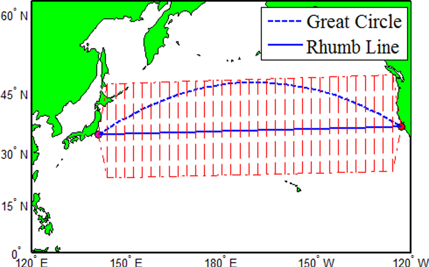
Figure 5. Extended sailing area based on Rhumb Line.

Figure 6. Extended sailing area based on custom route.
5.2. Population initialisation
To solve the minimum voyage time optimisation problem using a RCGA, it is necessary to represent each route in a chromosome form. Let us assume that the population size is M. Let vector lonpts represent the longitude information of the chromosome and vector latptsj represent the latitude information of the j-th chromosome. The longitude for each chromosome is the same, while the latitude for each chromosome should be within the range of LowerBound and UpperBound.
 $${{\bi lonpts}}=[\matrix{l_s & l_1 & \ldots & l_i & \ldots & l_d}], \quad i=\overline{1,n}$$
 $${{\bi latpts}}_{j} = [\matrix{\lambda_s & \lambda_{j1} & \ldots & \lambda_{ji} & \ldots & \lambda_d}], \quad i=\overline{1,n}; j=\overline{1,M}$$
The numbers of required chromosomes are randomly generated according to the population size. For example, one individual chromosome can be generated by Equation (24):
 $${{\bi latpts}}_1=rand(1,N)\times [{{\bi UpperBound}}-{{\bi LowerBound}}]^{\prime} + {{\bi LowerBound}}$$
where N is the dimension of the variables (the number of waypoints), rand(1, N) generates a random number vector with a length of N, which is uniformly distributed between 0 and 1.
5.3. Route calculation
Let us now consider the computational algorithm for the voyage time for the given route (r, v). Assume the following notations: t 0 is the departure time from the departure point (λs, l s), Δ T is the fixed time period of the weather forecast update interval, t̃ is the time interval between the last weather forecast update time and the departure time t 0, T voyage is the voyage time, T alarm is the alarm time and  $N_{num\_\Delta T}$ is the position where the weather forecast updated during the voyage.
We will first split each segment of the route into several small legs according to the grid size of meteorological data as shown in Figure 7. The meteorological data are considered the same for each small leg and remain unchanged for Δ T time. The actual speed for each small leg can be calculated using Equation (14) and the voyage time T voyage can be obtained using Equation (11). The meteorological data will be updated whenever  $T_{voyage}+\tilde{t}$ is a multiple of the time period Δ T, as shown by the green star point in Figure 7. Simultaneously, the voyage time of the small legs are marked as alarm time when the significant wave height is greater than a certain value (weather alarm zone), thus the T alarm can be calculated. Finally, the objective function value of the route can be calculated using Equation (12) and it is set to infinity no matter which small leg passes through the land obstacles or non-navigable areas.

Figure 7. Split route according to the grid size of meteorological data.
5.4. Fitness assignment
The fitness greatly influences the performance of the genetic algorithm, which is generally related to the objective function value. In the minimum value problem, the smaller the objective function value, the greater the fitness will be. It is not recommended to use the objective function as the fitness directly; thus, it is necessary to perform a certain scale transformation between the objective function and the fitness function. Linear scale transformation, power scale transformation and exponential scale transformation are some commonly used transformation methods.
In this paper, we first sort the individuals in descending order according to the objective function value. The fitness values are then assigned to each individual based on the sorted position. Individuals who rank in the front-row position have low fitness. Let vector J represent the objective function values of each individual, after calculating the objective function value for each route according to Equation (12):
 $${{\bi J}}=[\matrix{J_1 & \ldots & J_i & \ldots & J_M}]^{\prime}, \quad i=\overline{1,M}$$
where J i is the objective function value of i-th individual, and M is the population size.
Let pos i represent the position of the i-th individual after sorting in descending order; then, the fitness fit i of the i-th individual can be calculated using Equation (26):
 $$fit_i=2\times {pos_i-1 \over M-1}$$
The fitness value is linearly distributed according to the sorted position. The fitness of the individual in the top position (objective function is the largest) is 0, and the fitness of the individual in the last position (objective function is the smallest) is 2.
5.5. Selection operation
The selection operation is based on the fitness value of the individuals in the parent population to determine which individuals need to generate the offspring population. The greater the fitness of an individual, the greater the probability that this individual will produce the offspring population. In this paper, three selection operations are provided: roulette wheel selection, stochastic universal selection and tournament selection.
Roulette wheel selection is the simplest. This method first accumulates the fitness of each individual. Suppose that the accumulated value is fit sum. Individuals are mapped in a continuous interval [0, fit sum] in a one-to-one way and then they generate a pointer (random number) within the interval [0, fit sum] at the same probability. The individual is selected according to the range in which the pointer is located. If M individuals need to be selected, then M pointers need to be generated.
Stochastic universal selection is similar to roulette wheel selection. The difference is that this method produces M equidistant pointers at the same time. The first pointer ptr is generated at interval [0, fit sum/M], while the remaining M−1 pointers are as follows:
 $$[ptr,ptr+fit_{sum}/M,\ldots,ptr+(M-1)\times fit_{sum}/M]$$
Tournament selection first selects a small number of individuals from the population. An individual who has the highest fitness value will be selected to produce the offspring population. This operation is repeated until the number of offspring meets the requirements. Each selection method has its own characteristics. In this paper, different selection strategies are used in different subpopulations in order to achieve a different evolutionary strategy.
5.6. Recombination operation (Crossover)
A recombination operation is the main operation to generate new individuals. It combines two chromosomes to receive good genes from the parent to generate new individuals so that the population can gradually improve during evolution. The traditional one-point crossover introduced by Holland (Reference Holland1975) swaps the genes between the parents, starting from a point selected randomly from the chromosomes. There are expanded crossovers (Kang et al., Reference Kang, Choi, Kim and Park2012), such as the two-point crossover, k-point crossover, and uniform crossover; however, these methods are more suitable for binary coding. As a result of using the RCGA, an arithmetic operation is adopted to perform the recombination operation. Assuming that the two individuals who need to be crossed are latpts1t and latpts2t, the new individuals generated after the recombination operation can be expressed as follows:
 $$\left\{\matrix{{\bi latpts}_1^{t+1} = {\bf \alpha} \times ({\bi latpts}_2^{t})^{\prime} + (1-{\bf \alpha}) \times ({\bi latpts}_1^{t})^{\prime} \hfill \cr {\bi latpts}_2^{t+1}={\bf \alpha}\times ({\bi latpts}_1^{t})^{\prime} +(1-{\bf \alpha})\times ({\bi latpts}_2^{t})^{\prime} \hfill} \right.$$
where α is a vector parameter with a length of N, and each of its values is a uniform random number within a range. In this paper, the range is set to [−0.5, 1.5]. In the meantime, in order to ensure that the individuals obtained after the recombination operation are within the boundary, the individuals who exceed a boundary are placed on the nearest boundary.
5.7. Mutation operation
The main purpose of the mutation operator is to put the missing allele back into the population to produce a new solution while increasing the diversity of the population. A number of mutation methods have been applied to RCGAs: uniform mutation, boundary mutation, non-uniform mutation and Gaussian variation, each of which has its own characteristics. We present a hybrid mutation method that combines uniform and Gaussian mutations; that is, part of the subpopulation adopts the uniform mutation, and the other part adopts the Gaussian mutation. The genotypes of the subpopulations can be exchanged through the migration operation to increase the diversity of the population.
Uniform mutation replaces one or more original genes on the chromosome with a smaller probability by generating random numbers distributed uniformly within the boundary. The resulting mutation value is distributed throughout the constraint space evenly, which can effectively improve the diversity of the population. Let us assume that UpperBound i and LowerBound i are the upper bound and lower bound of the i-th coordinate, respectively. The new value lat′i produced by uniform mutation can be calculated by the following equation:
 $$lat_{i}^{\prime} = rand \times (UpperBound_i - LowerBound_i) + LowerBound_i$$
where rand generates a random number in interval [0,1] with the same probability.
Gaussian mutation replaces one or more original genes on the chromosome with a smaller probability by generating random numbers with expectation  $\bar{X}$ and variance σ2. Gaussian mutation can focus on searching local regions to find the optimal solution. Assuming that we need to perform a mutation operation for the lat i, then a Gaussian random number with expectation lat i and variance
  $0.005 \times (UpperBound_{i} - LowerBound_{i})$ can be generated to replace lat i.
5.8. Reinsert operation (elite retention strategy)
The reinsert operation inserts a certain percentage of the offspring population into the parent population according to the fitness value while removing individuals with lower fitness in the parent population; the new population will be the next parent population. The reinsert operation ensures that the elite individuals in the population are not eliminated while speeding up the convergence rate. The process of the reinsert operation is shown in Figure 8. First, the parent population and the offspring population are sorted in descending order according to fitness value. Then, individuals who ranked in the back-row position in parent population P t will be replaced by individuals who ranked in the front-row position in offspring population Q t, and the new population P t+1 will be the next parent population.

Figure 8. Reinsert operation illustration.
5.9. Migration operation
The migration operation exchanges individuals between each subpopulation of every certain generation. Each subpopulation can apply a different evolutionary strategy. The individuals with high fitness in the subpopulation are then passed to the other subpopulations through a migration operation, thus increasing the spread of good individuals among populations, accelerating the convergence rate and improving the accuracy of the solution. Individuals are either chosen randomly or based on fitness to perform migration.
In this paper, individuals who have higher fitness will be chosen to perform migration operations according to migration probability. The structure of migration can be network topology, ring topology and adjacency topology. In this paper, a cyclic ring topology is chosen, as shown in Figure 9. The individuals in subpopulation 1 migrate to subpopulation 2, and the individuals in subpopulation 2 migrate to subpopulation 3, and so on.

Figure 9. Cyclic ring topology illustration.
6. EXPERIMENTAL RESULTS
In this section three examples are presented to verify the applicability of the proposed algorithm. The first focuses on finding a shortest route without considering any weather constraints to test the basic performance of the present algorithm. The second concentrates on searching a minimum voyage time route under bad weather conditions and land obstacles constraints. The last gives an example of using a custom reference route to establish the sailing area to find a minimum voyage time route. The implementation of the proposed algorithms is realised in a Matlab environment on a PC machine (AMD FX-6300 Six-core 3.5GHZ, RAM 4GB).
The container ship type S-175 (Zhang et al., Reference Zhang, Lu, Cai and Shi2005), with a standard displacement of 23,740 tonnes, was chosen to perform the simulation experiment for route optimisation. In all examples, the genetic algorithm parameters were set as follows: the number of subpopulations was six, the size of the subpopulation was 20, the mutation probability was 0.05, the migration probability was 0.2, the migration interval was 20 generations, the reinsertion rate was 0.9, the generation gap was 0.8 and the maximum number of iterations was 1,000.
The meteorological data used in this research were previously ascertained from the European Medium Weather Forecast Centre. The meteorological data included “10-metre U wind component”, “10-metre V wind component”, “Mean wave direction” and “Significant height of combined wind, waves and swell”. The grid size of the meteorological data was  $1^{\circ} \times 1^{\circ}$. The forecasted data in a single file covers ten days. If a forecasted ship passage time was longer than ten days, it was assumed that the weather conditions remained the same as that of the last day (the tenth day) for the excess time. The update interval of the data is six hours, updating at 00:00, 06:00, 12:00 and 18:00 every day.
6.1. Example 1 - Tokyo Harbour (35° N, 141° E) to San Francisco City (37° N, 123° W), departure time 2016.01.10 00:00:00
In general, the route obtained by the algorithm does not have an absolute evaluation criteria due to the impact of meteorological conditions. The shortest path between two points on a sphere is the great circle route. Hence, we first solve the shortest route problem without considering any weather constraints to test the basic performance of the present algorithm. According to the great circle route distance formula, the distance between the above two points is 4,438.82 nautical miles, which is the shortest path length. We ran the proposed algorithm ten times to calculate the optimum route; the results are shown in Table 1. The average execution time is 92 seconds.
Table 1. Optimum route distance.

From Table 1, we can see that the average length of the results has a difference of 2.87 nautical miles and relative error of 0.065% compared with the great circle route distance. Therefore, the performance of the algorithm has some reliability.
6.2. Example 2 - Tokyo Harbour (35° N, 141° E) to San Francisco City (37° N, 123° W), departure time 2016.01.10 00:00:00
In this example, we aim to search for a minimum voyage time route under bad weather and land obstacles constraints. The optimisation constraint set includes the following: land obstacles; external borders of the sailing area (by increasing and decreasing of the latitude of the rhumb line waypoints by 12°); and regions where the forecasted significant wave height is above 5 metres (a dynamic constraint). The calm water set speed is in the range of 10 to 25 knots. The latitude range was chosen as  $[0^{\circ}\,N, 62^{\circ}\,N]$ and the longitude range was chosen as
  $[120^{\circ}\,E, 120^{\circ}\,W]$.
Ship performance was simulated under the output power required to maintain a navigation speed of 22 knots in calm water for all segments. The obtained optimised route is shown in Figure 10. The execution time was 154 seconds. The distance of the optimised route was 5,215.41 nautical miles, and the voyage time was 276.291 hours with an alarm time of 0 hours. The distance of the great circle route was 4,438.82 nautical miles, and the voyage time was 248.848 hours with the alarm time 87.571 hours under the same meteorological data. The distance of the rhumb line route was 4,664.14 nautical miles, and the voyage time was 275.755 hours with an alarm time of 119.532 hours under the same meteorological data. The voyage time of the optimised route is larger than the great circle route and the rhumb line. However, the alarm time was 0 hours, which indicates that it chose to travel longer routes to bypass dangerous areas to ensure safety.

Figure 10. Route simulation results.
The best and the average objective function value for each generation are shown in Figure 11. We can see that the algorithm converges after approximately 200 generations. The comparisons of the actual voyage speed, the heading angle and the significant wave height among these three routes are shown in Figures 12, 13 and 14, respectively. From these figures, it can be seen that the optimum route has a lower significant wave height (no more than 5 metres) compared to the other routes. As a result, the optimised route succeeded in reducing the additional resistance, thereby reducing the ship speed loss.

Figure 11. Genetic algorithm performance curve.

Figure 12. Comparison of the actual speed.

Figure 13. Comparison of heading angle.

Figure 14. Comparison of the wave height.
Figure 15 shows snapshots of the optimised route at different voyage times. From it we can see that the optimised route can effectively avoid the areas with significant wave height larger than 5 metres (alarm zone) and choose areas with low significant wave height.

Figure 15. Snapshot of the optimised route at different voyage times.
6.3. Example 3 – Saint-Denis (20.9° S, 55.5° E) to St. Helena (15.97° S, 5.71° W), departure time 2016.01.01 00:00:00
In this example, the great circle route and rhumb line between the two points pass through land obstacles. Thus, we establish the sailing area by extending a customised reference route. The optimisation constraint set includes the following: land obstacles; external borders of the sailing area (by increasing and decreasing the latitude by 10° of the reference route waypoints); and regions where the forecasted significant wave height is above 5 metres (a dynamic constraint); the calm water set speed is in the range of 10 to 25 knots. The latitude range was chosen as  $[0^{\circ}\,S, 50^{\circ}\,S]$, and the longitude range was chosen as
  $[10^{\circ}\,W, 60^{\circ}\,E]$.
Ship performance was simulated under the output power required to maintain a navigation speed of 22 knots in calm water for all segments. The obtained optimised route is shown in Figure 16. The execution time was 112 seconds. The distance of the optimised route was 3,883.69 nautical miles, and the voyage time was 194.455 hours with alarm time 0 hours. Figure 17 shows snapshots of the optimised route at different voyage times. It can be seen from this figure that the optimised route can effectively avoid the land obstacles without increasing the distance too greatly.
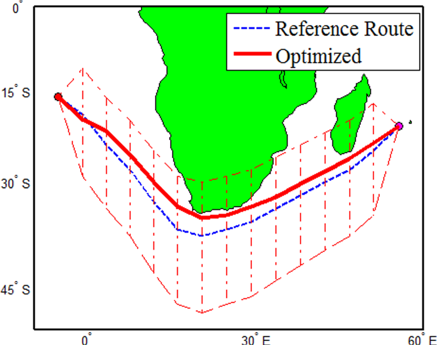
Figure 16. Route simulation results.

Figure 17. Snapshots of the optimised route at different voyage times.
7. CONCLUSIONS
Ship weather routing has significant economic and practical value in ship safety and operating costs. Therefore, new and effective decision-making tools should be applied to ship navigation as the maritime industry develops. Such tools not only enable route planning automation but also provide a reference for decision-making in route planning. In this paper, a real-coded genetic algorithm is proposed to provide decision-making for ship weather routing. Experimental results show that the algorithm can minimise the voyage time and provide a route that does not intersect with dangerous areas, which indicates that it can avoid dangers to some extent. Previous studies have considered multiple optimisation types, such as minimum fuel consumption, minimum voyage time and minimum total distance. In contrast, here we have only taken minimum voyage time as the optimisation criterion, but this method has the potential to consider other types of criteria. Our future research will focus on including the effects of the multi-objective factors while constructing an optimal route. We will also investigate applying a safety distance to the route to ensure separation from dangers.
FINANCIAL SUPPORT
The reported study has been funded by RFBR (Russian Foundation for Basic Research) according to research project number 17-07-00361a.


