2.1. Physical model and numerical settings

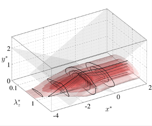
The sketch of the physical model and computational domain is depicted in figure 1. We simulate the fully-developed supersonic turbulent boundary layer impinged by an oblique shock wave. The mean velocity profile of the incoming turbulence is described according to Musker (Reference Musker1979), and the velocity fluctuations are generated by the synthetic digital filtering approach (Klein, Sadiki & Janicka Reference Klein, Sadiki and Janicka2003). The mean temperature and temperature fluctuations are given according to the generalized Reynolds analogy (Zhang et al. Reference Zhang, Bi, Hussain and She2014). The oblique shock is generated at the top boundary by imposing the inviscid Rankine–Hugoniot jump condition to simulate the effect of a wedge shock generator with deflection angle $8^{\circ }$. The generated shock angle is $33.2^{\circ }$, and the impingement point is $x_{imp}=30\delta _{in}$ (where $\delta _{in}$ is the nominal boundary layer thickness at the inlet). The upper and outflow boundaries are enforced by non-reflecting conditions (Pirozzoli & Colonius Reference Pirozzoli and Colonius2013). At the lower wall, no-slip and no-penetration conditions are applied for velocity, and the isothermal condition is applied for temperature, with the wall temperature set as the recovery temperature $T_w=1.92 T_\infty$ to achieve a quasi-adiabatic thermal boundary condition. Periodic conditions are applied in the spanwise direction.

Figure 1. Sketch of physical model and computational domain.

We solve directly the three-dimensional Navier–Stokes equations for compressible Newtonian gas with the finite difference method. The DNS are performed with the open-source ‘STREAmS’ solver developed by Bernardini et al. (Reference Bernardini, Modesti, Salvadore and Pirozzoli2021), which has been validated widely for solving compressible channel, boundary layer, and especially OSBLI flows (e.g. Bernardini et al. Reference Bernardini, Asproulias, Larsson, Pirozzoli and Grasso2016; Volpiani, Bernardini & Larsson Reference Volpiani, Bernardini and Larsson2020). The convective terms are approximated by the sixth-order kinetic-energy-preserving scheme (Pirozzoli Reference Pirozzoli2010), and switched to the fifth-order WENO scheme (Jiang & Shu Reference Jiang and Shu1996) near strong flow compression, which is identified by the criterion of Ducros et al. (Reference Ducros, Ferrand, Nicoud, Weber, Darracq, Gacherieu and Poinsot1999). The viscous terms are cast as Laplacian forms and approximated by the sixth-order central difference scheme. Time advancement is achieved by Wray's three-stage third-order scheme (Wray Reference Wray1990).

The free-stream Mach number of the inflow is set as $M_\infty = 2.28$, and the Reynolds number is set as $Re_{in}= \rho _\infty U_\infty \delta _{in} / \mu _\infty =12\,000$, with $\rho _\infty$, $U_\infty$ and $\mu _\infty$ denoting the free-stream density, velocity and dynamic viscosity coefficients, and $\delta _{in}$ the nominal thickness of the incoming boundary layer. The sizes of the computational domain in the streamwise ($x$), wall-normal ($y$) and spanwise ($z$) directions are $(L_x, L_y, L_z) = (60 \delta _{in}, 12 \delta _{in}, 6.5 \delta _{in})$, respectively. The computational domain is discretized by $(2000, 320, 240)$ grids in the three directions. The grids are uniformly distributed in the $x$ and $z$ directions, with the mesh intervals under the viscous scales (defined below) being $\Delta x^{+} \approx 5.4$ and $\Delta z^{+} \approx 4.9$. In the wall-normal direction, the grids are stretched by a hyperbolic-sine function within $y=2.5\delta _{in}$, with the first off-wall grid located at $\Delta y^{+}_w \approx 0.7$, and uniformly distributed above it, with grid interval $\Delta y^{+} \approx 7.0$. According to the DNS performed by Volpiani, Bernardini & Larsson (Reference Volpiani, Bernardini and Larsson2018) under roughly the same flow parameters and numerical conditions, the grid intervals in the present study are fine enough to obtain accurate results.

The statistics are averaged in the spanwise direction with 900 instantaneous flow fields over the period $600 \delta _{in} / U_\infty$. To further obtain smoother statistics, the average in the streamwise direction is also adopted across 11 grids, within which the streamwise variation of the mean flow is insignificant, even inside the interaction zone. The ensemble average of a generic variable $\varphi$ is denoted as $\bar \varphi$, and the corresponding fluctuation by $\varphi '$, the density-weighted average (or Favre average) by $\tilde \varphi$, and the corresponding fluctuation $\varphi ''$.

2.2. Basic flow statistics and validation

We take the streamwise location at $x=15.0 \delta _{in}$ as the reference plane (denoted by $x_0$), where the turbulence is free from the impact of the impinging shock wave. The statistical properties at $x_0$ (hereinafter denoted by the subscript $0$) are listed in table 1. The friction Reynolds number $Re_\tau$ is defined as

(2.1)\begin{equation} Re_\tau = \frac{\rho_w u_\tau \delta_0} {\mu_w}, \end{equation}

with

(2.2a,b)\begin{equation} u_\tau = \sqrt{\frac{\tau_w}{\rho_w}},\quad \tau_w = \left.\mu_w\,\frac{\partial \bar u}{\partial y } \right|_w, \end{equation}

where $\rho _w$ and $\mu _w$ denote the mean density and dynamic viscosity on the wall, and $\tau _w$ denotes the mean wall shear stress. The displacement and momentum thicknesses, denoted as $\delta ^{*}$ and $\theta$, are defined as

(2.3a,b)\begin{equation} \delta^{*} = \int_0^{\delta} \left( 1- \frac{\bar \rho \bar u} {\rho_\infty U_\infty} \right) {\rm d} y,\quad \theta = \int_0^{\delta} \frac{\bar \rho \bar u}{\rho_\infty U_\infty} \left( 1- \frac{\bar u}{ U_\infty} \right) {\rm d} y . \end{equation}

The incompressible boundary layer thicknesses, denoted by $\delta ^{*}_i$ and $\theta _i$, along with the incompressible shape factor $H_i$, are defined accordingly by setting the mean density ratio as unity.

Table 1. Statistical properties at the reference plane $x=15.0 \delta _{in}$. Here, $C_f = 2 \tau _w / (\rho _\infty U^{2}_\infty )$, $Re_{\theta 0} = \rho _\infty U_\infty \theta _0 / \mu _\infty$, $Re_{\delta 2, 0} = \rho _\infty U_\infty \theta _0 / \mu _w$, $H_0 = \delta ^{*}_0 / \theta _0$ and $H_{i0} = \delta ^{*}_{i0} / \theta _{i0}$.

The van-Driest-transformed mean velocity and Reynolds stress under viscous scales in (2.2a,b) are defined as

(2.4a,b)\begin{equation} u^{+}_{VD} = \int^{\bar u^{+}}_0 \sqrt{\frac{\bar \rho}{ \rho_w}}\,{\rm d} \bar u^{+},\quad R^{*}_{ij} = \frac{\overline{\rho u''_i u''_j}}{\tau_w}, \end{equation}

where the superscript $+$ represents the normalization by $u_\tau$ as incompressible flows. The distributions at $x_0$ are displayed in figure 2 against the wall-normal coordinate under viscous scale $y^{+}=y\,Re_\tau /\delta _0$, and compared with those of supersonic turbulent boundary layers at $M_\infty =2.0$ and $Re_\tau \approx 200$ reported by Pirozzoli & Bernardini (Reference Pirozzoli and Bernardini2011b). The wall-normal distributions of both the mean velocity and Reynolds stress in the present study agree reasonably well with the reference, indicating the validity of the current results. It also suggests that the turbulence at the reference station $x_0$ is fully developed.

Figure 2. Wall-normal distributions of (a) van-Driest-transformed mean velocity and (b) Reynolds stress. Lines indicate results at $x_0=15 \delta _{in}$; symbols indicate reference data in Pirozzoli & Bernardini (Reference Pirozzoli and Bernardini2011b) at $M_0 =2.0$, $Re_\tau \approx 200$.

We further report the skin friction coefficient $C_f$ and mean wall pressure $\bar p_w$ distribution along the streamwise ($x$) direction, with the former defined as

(2.5)\begin{equation} C_f = \frac{2\tau_w}{\rho_\infty U^{2}_\infty}. \end{equation}

The subsequent results will be reported under the scaled interaction coordinate, i.e. $x^{*} = (x-x_{imp})/\delta _0$ and $y^{*}=y/\delta _0$, as usually adopted in SBLI flow analysis. The streamwise distribution of $C_f$ is presented in figure 3(a). It can be identified that the streamwise locations of the flow separation and reattachment points are $x^{*}_s \approx -2.60$ and $x^{*}_r \approx -0.73$, where $C_f=0$. The extrapolated origin of the reflected shock in the mean velocity field is located at $x^{*}_i \approx -3.27$. Therefore, the lengths of the interaction and separation zones are $L^{*}_{int} = x^{*}_i \approx 3.27$ and $L^{*}_{sep} = x^{*}_r - x^{*}_s \approx 1.87$, respectively. These values are consistent with the results reported in Volpiani et al. (Reference Volpiani, Bernardini and Larsson2018, figure 12). The mean wall pressure $\bar p_w$ distribution is presented in figure 3(b), along with the DNS results reported by Pirozzoli & Bernardini (Reference Pirozzoli and Bernardini2011a) and the inviscid theory. The presently obtained result generally collapses with the reference data. The wall pressure increases rapidly at the start of the interaction zone and gradually reaches the theoretical inviscid solution. The preceding results confirmed the accuracy of the present DNS statistics.

Figure 3. Wall statistics: (a) skin friction $C_f$, (b) mean pressure $\bar p_w$. Red symbols indicate reference data from Pirozzoli & Bernardini (Reference Pirozzoli and Bernardini2011a); blue dashed lines indicate the inviscid solution; $x_i$, $x_s$ and $x_r$ are the locations of the extrapolated origin of the reflected shock, the separation and the reattachment point, respectively.

3.1. Two-point correlation transport equation

We first derive the transport equation of spanwise two-point correlation, considering the statistical homogeneity and periodicity in that direction. According to Arun et al. (Reference Arun, Sameen, Srinivasan and Girimaji2021), the fluctuation of momentum equation can be cast as

(3.1)\begin{align} &\frac{\partial \rho u''_i}{\partial t}+\frac{\partial \rho u''_i (\tilde u_k + u''_k)}{\partial x_k} +\rho u''_k\,\frac{\partial \tilde u_i}{\partial x_k}\nonumber\\ &\quad ={-}\frac{\partial p'}{\partial x_i} + \frac{\partial \tau'_{ik}}{\partial x_k} +\left( 1-\frac{\rho}{\bar \rho} \right) \left( -\frac{\partial \bar p}{\partial x_i}+ \frac{\partial \bar \tau_{ik}}{\partial x_k}\right) +\frac{\rho}{\bar \rho}\,\frac{\partial \bar \rho R_{ik}}{\partial x_k}. \end{align}

Note that this equation is obtained by combining the fluctuation of momentum equation in non-conservative form and the continuity equation. The spanwise two-point correlation tensor between velocity components $u''_i$ at $\boldsymbol {x} = (x,y,z)$ and $u''_j$ at $({\boldsymbol x+ \boldsymbol r})=(x,y,z+r_z)$ is defined as (Arun et al. Reference Arun, Sameen, Srinivasan and Girimaji2021)

(3.2)\begin{equation} Q_{ij}(\boldsymbol x,\boldsymbol r)=\frac{1}{2}\,\overline{(\rho(\boldsymbol x)+\rho(\boldsymbol x+ \boldsymbol r))\,u''_i(\boldsymbol x)\,u''_j(\boldsymbol x+ \boldsymbol r)}, \end{equation}

which is a function of $x$, $y$ and $r_z$. The derivation of the $Q_{ij}$ transport equation is similar to that in the incompressible flows. The derivatives in the $z$ direction at $\boldsymbol x$ and $\tilde {\boldsymbol x} = \boldsymbol x + \boldsymbol r$ are related by $r_z$ (Lee & Moser Reference Lee and Moser2019):

(3.3a,b)\begin{equation} \frac{\partial }{\partial z} ={-} \frac{\partial}{\partial r_z},\quad \frac{\partial }{\partial \tilde z} = \frac{\partial}{\partial r_z}. \end{equation}

Moreover, the averaged flow quantities are independent of $r_z$, i.e.

(3.4a,b)\begin{equation} \bar \varphi(\boldsymbol x) = \bar \varphi (\boldsymbol x + \boldsymbol r),\quad \tilde \varphi(\boldsymbol x) = \tilde \varphi (\boldsymbol x + \boldsymbol r). \end{equation}

After a detailed derivation, we formulate the transport equation for two-point correlation tensor as

(3.5)\begin{equation} \frac{\partial Q_{ij}(\boldsymbol x, \boldsymbol r)}{\partial t} = C_{ij} + P_{ij} + D_{ij} + \varPi_{ij} + \varepsilon_{ij} + T_{ij} + B_{ij}. \end{equation}

The terms on the right-hand side represent the contributions from the mean flow convection, production, diffusion, pressure-strain, viscous dissipation, inter-scale transfer and mass-diffusion, respectively. The convection and production terms are related to the variation of mean velocity:

(3.6)\begin{gather} C_{ij} ={-} \frac{\partial}{\partial x_k} Q_{ij}(\boldsymbol x,\boldsymbol r)\,\tilde u_k(\boldsymbol x)\quad (k=1,2), \end{gather}

(3.7)\begin{gather} P_{ij} ={-} Q_{kj}(\boldsymbol x,\boldsymbol r)\,\frac{\partial \tilde u_i(\boldsymbol x)}{\partial x_k} - Q_{ik}\,(\boldsymbol x,\boldsymbol r) \frac{\partial \tilde u_j(\boldsymbol x)}{\partial x_k}\quad (k=1,2). \end{gather}

The diffusion term $D_{ij}$ involves the diffusion by turbulent transport $D^{T}_{ij}$, pressure fluctuation $D^{P}_{ij}$, and viscous stress fluctuation $D^{V}_{ij}$:

(3.8)\begin{gather} D^{T}_{ij} ={-} \frac{1}{4}\,\frac{\partial}{\partial x_k} \overline{(\rho(\boldsymbol x)+\rho(\boldsymbol x+ \boldsymbol r))\,u''_i(\boldsymbol x)\,u''_j(\boldsymbol x+ \boldsymbol r)\, (u''_k(\boldsymbol x)+u''_k(\boldsymbol x+ \boldsymbol r ))}\quad (k=1,2), \end{gather}

(3.9)\begin{gather} D^{P}_{ij} ={-} \frac{1}{2} \left( \overline{ \left( 1 + \frac{\rho(\boldsymbol x+\boldsymbol r)}{\rho(\boldsymbol x)}\right) \frac{\partial p'(\boldsymbol x)\,u''_j(\boldsymbol x+\boldsymbol r)}{\partial x_k}}\,\delta_{ik}\right.\nonumber\\ \left.\qquad\qquad + \overline{ \left( 1 + \frac{\rho(\boldsymbol x)}{\rho(\boldsymbol x+ \boldsymbol r)}\right) \frac{\partial p'(\boldsymbol x+ \boldsymbol r)\,u''_i(\boldsymbol x)}{\partial x_k}}\,\delta_{jk} \right), \end{gather}

(3.10)\begin{gather} D^{V}_{ij} = \frac{1}{2} \left( \overline{\left( 1 + \frac{\rho(\boldsymbol x+\boldsymbol r)}{\rho(\boldsymbol x)}\right) \frac{\partial \tau'_{ik}(\boldsymbol x)\,u''_j(\boldsymbol x+ \boldsymbol r)}{\partial x_k}}\right. \nonumber\\ \left.\qquad\qquad\qquad\qquad\qquad + \overline{\left( 1 + \frac{\rho(\boldsymbol x)}{\rho(\boldsymbol x+\boldsymbol r)}\right) \frac{\partial \tau'_{jk}(\boldsymbol x+ \boldsymbol r)\,u''_i(\boldsymbol x)}{\partial x_k}} \right)\quad (k=1,2). \end{gather}

The pressure-strain term $\varPi _{ij}$ reflects the inter-component energy transfer:

(3.11)\begin{align} \varPi_{ij} = \frac{1}{2} \left( \overline{ \left(1 + \frac{\rho(\boldsymbol x+ \boldsymbol r)}{\rho(\boldsymbol x)}\right) p'(\boldsymbol x)\,\frac{\partial u''_j(\boldsymbol x+ \boldsymbol r)}{\partial x_i}} + \overline{ \left(1 + \frac{\rho(\boldsymbol x)}{\rho(\boldsymbol x+ \boldsymbol r)}\right) p'(\boldsymbol x+ \boldsymbol r)\,\frac{\partial u''_i(\boldsymbol x)}{\partial x_j}} \right) . \end{align}

The dissipation by viscosity $\varepsilon _{ij}$ is expressed as

(3.12)\begin{align} \varepsilon_{ij} &={-} \frac{1}{2} \left( \overline{ \left(1 + \frac{\rho(\boldsymbol x+ \boldsymbol r)}{\rho(\boldsymbol x)}\right) \tau'_{ik}(\boldsymbol x)\,\frac{\partial u''_j(\boldsymbol x+ \boldsymbol r)}{\partial x_k}} \right.\nonumber\\ &\quad \left.+ \overline{\left(1 + \frac{\rho(\boldsymbol x)}{\rho(\boldsymbol x+\boldsymbol r)}\right) \tau'_{jk}(\boldsymbol x+\boldsymbol r)\,\frac{\partial u''_i(\boldsymbol x)}{\partial x_k}} \right)\quad (k=1,2,3). \end{align}

The inter-scale energy transfer, corresponding to the nonlinear turbulent interactions in incompressible flows (Domaradzki et al. Reference Domaradzki, Liu, Härtel and Kleiser1994; Mizuno Reference Mizuno2016; Lee & Moser Reference Lee and Moser2019), can be split as $T_{ij}=T^{xy}_{ij}+T^{z}_{ij}$, where

(3.13)\begin{align} T^{xy}_{ij} &={-} \frac{1}{2}\,\overline{u''_j(\boldsymbol x+\boldsymbol r)\,\frac{\partial \rho(\boldsymbol x)\,u''_i(\boldsymbol x)\,u''_k(\boldsymbol x)}{\partial x_k}} - \frac{1}{2}\, \overline{\rho(\boldsymbol x+\boldsymbol r)\,u''_j(\boldsymbol x+\boldsymbol r)\,u''_k(\boldsymbol x)\, \frac{\partial u''_i (\boldsymbol x)}{\partial x_k}}\nonumber\\ &\quad - \frac{1}{2}\,\overline{u''_i(\boldsymbol x)\,\frac{\partial \rho(\boldsymbol x+\boldsymbol r)\,u''_j(\boldsymbol x+\boldsymbol r)\,u''_k(\boldsymbol x+\boldsymbol r)}{\partial x_k}} - \frac{1}{2}\,\overline{\rho(\boldsymbol x)\,u''_i(\boldsymbol x)\,u''_k(\boldsymbol x+\boldsymbol r)\, \frac{\partial u''_j(\boldsymbol x+\boldsymbol r)}{\partial x_k}}\nonumber\\ &\quad -D^{T}_{ij}\quad (k=1,2), \end{align}

(3.14)\begin{align} T^{z}_{ij}&={-} \frac{1}{2}\,\frac{\partial }{\partial r_z} \overline{(\rho(\boldsymbol x)+ \rho(\boldsymbol x+ \boldsymbol r))\,u''_i(\boldsymbol x)\,u''_j(\boldsymbol x + \boldsymbol r)\, (w''(\boldsymbol x+ \boldsymbol r)-w''(\boldsymbol x)) }\nonumber\\ &\quad - \frac{1}{2}\,\overline{u''_i (\boldsymbol x)\,u''_j (\boldsymbol x+\boldsymbol r)\, \frac{\partial}{\partial r_z} \left( \rho(\boldsymbol x)\,w''(\boldsymbol x+\boldsymbol r) -\rho(\boldsymbol x + \boldsymbol r)\,w''(\boldsymbol x) \right)}. \end{align}

Complicated as it is, we can easily prove that $T_{ij} \rightarrow 0$ at the limit of $r_z \rightarrow 0$, indicating that this term is responsible only for the inter-scale energy transfer. Finally, the mass-diffusion $B_{ij}$, caused by the density fluctuation, can be cast as

(3.15)\begin{align} B_{ij} &= \frac{1}{2}\left( \overline{u''_j(\boldsymbol x+\boldsymbol r)} - \frac{\overline{\rho(\boldsymbol x)\,u''_j(\boldsymbol x+\boldsymbol r)}}{\bar \rho (\boldsymbol x)} + \overline{\frac{\rho(\boldsymbol x+ \boldsymbol r)\,u''_j(\boldsymbol x+\boldsymbol r)}{\rho (\boldsymbol x)}} \right) \left( -\frac{\partial \bar p}{\partial x _i} + \frac{\partial \bar \tau_{ik}}{\partial x_k} \right)\nonumber\\ &\quad + \frac{1}{2} \left( \overline{u''_i(\boldsymbol x)} - \frac{\overline{\rho(\boldsymbol x + \boldsymbol r)\,u''_i(\boldsymbol x)}}{\bar \rho(\boldsymbol x)} + \overline{\frac{\rho(\boldsymbol x)\,u''_i(\boldsymbol x)}{\rho (\boldsymbol x + \boldsymbol r)}} \right) \left( -\frac{\partial \bar p}{\partial x _j} + \frac{\partial \bar \tau_{jk}}{\partial x_k} \right)\nonumber\\ &\quad - \frac{1}{2} \left( \frac{\overline{\rho(\boldsymbol x)\,u''_j(\boldsymbol x+\boldsymbol r)}}{\bar \rho(\boldsymbol x)} + \overline{\frac{\rho(\boldsymbol x+ \boldsymbol r) u''_j(\boldsymbol x+\boldsymbol r)}{\rho (\boldsymbol x)}} \right) \frac{\partial \bar \rho R_{ik}}{\partial x _k}\nonumber\\ &\quad - \frac{1}{2} \left( \frac{\overline{\rho(\boldsymbol x + \boldsymbol r)\,u''_i(\boldsymbol x)}}{\bar \rho(\boldsymbol x)} + \overline{\frac{\rho(\boldsymbol x)\,u''_i(\boldsymbol x)}{\rho (\boldsymbol x + \boldsymbol r)}} \right) \frac{\partial \bar \rho R_{jk}}{\partial x _k}. \end{align}

The equations above degenerate to the TKE transport equation by taking $r_z =0$ and contracting the indices $i$ and $j$, and to the two-point correlation transport equation for incompressible flows by taking the density as unity.

3.2. Spectra of Reynolds stress transport

As customarily performed in the incompressible turbulence (e.g. Lee & Moser Reference Lee and Moser2015), the transport equation of the Reynolds stress spectra can be obtained by performing a Fourier transform on the two-point correlation transport equation. According to the definition in (3.2), the spectra of the Reynolds stress tensor can be expressed as

(3.16)\begin{equation} \hat{Q}_{ij}= \mathrm{Re} \left[ \widehat{\rho u''_i}\,\widehat{u''_j}^{{\star}} + \widehat{u''_i}\,\widehat{\rho u''_j}^{{\star}} \right], \end{equation}

where the hat symbol denotes Fourier spectral coefficients, the superscript $\star$ indicates the complex conjugate, and $\mathrm {Re}$ represents taking the averaged real part. The budget terms of (3.5) are transformed into spectral space accordingly. The convection and production terms in (3.6) and (3.7) are therefore transformed as

(3.17)\begin{align}& \hat{C}_{ij} ={-} \frac{\partial}{\partial x_k} \hat{Q}_{ij} \tilde u_k, \end{align}

(3.18)\begin{align} &\hat{P}_{ij} ={-} \hat{Q}_{kj}\,\frac{\partial \tilde u_i}{\partial x_k} - \hat{Q}_{ik}\, \frac{\partial \tilde u_j}{\partial x_k}. \end{align}

The other budget terms are nonlinear, primarily due to the density variation. Taking the turbulent diffusion term $D^{T}_{ij}$ in (3.8) as an example, we reformulate all of those terms according to the independent variable

(3.19)\begin{align} D^{T}_{ij} & ={-} \frac{1}{4}\,\frac{\partial}{\partial x_k} ( \overline{\rho(\boldsymbol x)\, u''_i(\boldsymbol x)\,u''_k(\boldsymbol x)\,u''_j(\boldsymbol x+ \boldsymbol r) } + \overline{u''_i(\boldsymbol x)\,u''_k(\boldsymbol x)\,\rho(\boldsymbol x+ \boldsymbol r)\, u''_j(\boldsymbol x+ \boldsymbol r) }\nonumber\\ &\quad + \overline{\rho(\boldsymbol x)\,u''_i(\boldsymbol x)\,u''_j(\boldsymbol x+ \boldsymbol r)\,u''_k(\boldsymbol x+ \boldsymbol r)} + \overline{u''_i(\boldsymbol x)\,\rho(\boldsymbol x+ \boldsymbol r)\,u''_j(\boldsymbol x+ \boldsymbol r)\,u''_k(\boldsymbol x+ \boldsymbol r)} ), \end{align}

therefore its Fourier transform is expressed as

(3.20)\begin{equation} \hat{D}^{T}_{ij} ={-} \frac{1}{4}\,\frac{\partial}{\partial x_k} \mathrm{Re} \left[ \widehat{\rho u''_i u''_k}\, \widehat{u''_j}^{{\star}} + \widehat{u''_i u''_k}\,\widehat{\rho u''_j}^{{\star}} +\widehat{\rho u''_i}\, \widehat{u''_j u''_k}^{{\star}} + \widehat{u''_i}\,\widehat{\rho u''_j u''_k}^{{\star}} \right]. \end{equation}

The pressure diffusion, viscous diffusion, pressure-strain and viscous dissipation terms in (3.9), (3.10), (3.11) and (3.12) are correspondingly transformed as

(3.21)\begin{align} \hat{D}^{P}_{ij} &={-} \frac{1}{2}\,\mathrm{Re} \left[ \widehat{\frac{\partial p'}{\partial x_i}}\, \widehat{u''_j}^{{\star}} + \widehat{\frac{\partial p'}{\partial x_j}}^{{\star}}\,\widehat{u''_i} + \widehat{p'}\,\widehat{\frac{\partial u''_j}{\partial x_i}}^{{\star}} + \widehat{p'}^{{\star}}\, \widehat{\frac{\partial u''_i}{\partial x_j}} \right] \nonumber\\ &\quad - \frac{1}{2}\,\mathrm{Re} \left[ \widehat{\frac{1}{\rho}\,\frac{\partial p'}{\partial x_i}}\, \widehat{\rho u''_j}^{{\star}} + \widehat{\frac{1}{\rho}\,\frac{\partial p'}{\partial x_j}}^{\star}\, \widehat{\rho u''_i} + \widehat{\frac{p'}{\rho}}\,\widehat{\rho\,\frac{\partial u''_j}{\partial x_i}}^{{\star}} + \widehat{\frac{p'}{\rho}}^{{\star}}\,\widehat{\rho\,\frac{\partial u''_i}{\partial x_j}} \right], \end{align}

(3.22)\begin{align} \hat{D}^{V}_{ij} &= \frac{1}{2}\,\mathrm{Re} \left[ \widehat{\frac{\partial \tau'_{ik}}{\partial x_k}}\, \widehat{u''_j}^{{\star}} + \widehat{\frac{\partial \tau'_{jk}}{\partial x_k}}^{{\star}}\,\widehat{u''_i} + \widehat{\tau'_{ik}}\,\widehat{\frac{\partial u''_j}{\partial x_k}}^{{\star}} + \widehat{\tau'_{jk}}^{{\star}}\,\widehat{\frac{\partial u''_i}{\partial x_k}} \right] \nonumber\\ &\quad + \frac{1}{2}\,\mathrm{Re} \left[ \widehat{\frac{1}{\rho}\,\frac{\partial \tau'_{ik}}{\partial x_k}}\, \widehat{\rho u''_j}^{{\star}} + \widehat{\frac{1}{\rho}\,\frac{\partial \tau'_{jk}}{\partial x_k}}^{\star}\,\widehat{\rho u''_i} + \widehat{\frac{\tau'_{ik}}{\rho}}\,\widehat{\rho\,\frac{\partial u''_j}{\partial x_k}}^{{\star}} + \widehat{\frac{\tau'_{jk}}{\rho}}^{{\star}}\,\widehat{\rho\,\frac{\partial u''_i}{\partial x_k}} \right], \end{align}

(3.23)\begin{align} \hat{\varPi}_{ij} &= \frac{1}{2}\,\mathrm{Re} \left[ \widehat{p'}\,\widehat{\frac{\partial u'_{j}}{\partial x_i}}^{{\star}} + \widehat{p'}^{{\star}}\,\widehat{\frac{\partial u'_{i}}{\partial x_j}} + \widehat{\frac{p'}{\rho}}\,\widehat{\rho\,\frac{\partial u'_{j}}{\partial x_i}}^{{\star}} + \widehat{\frac{p'}{\rho}}^{{\star}}\,\widehat{\rho\,\frac{\partial u'_{i}}{\partial x_j}} \right], \end{align}

(3.24)\begin{align} \hat{\varepsilon}_{ij} &={-} \frac{1}{2}\,\mathrm{Re} \left[ \widehat{\tau'_{ik}}\,\widehat{\frac{\partial u'_{j}}{\partial x_k}}^{{\star}} + \widehat{\tau'_{jk}}^{{\star}}\,\widehat{\frac{\partial u'_{i}}{\partial x_k}} + \widehat{\frac{\tau'_{ik}}{\rho}}\,\widehat{\rho\,\frac{\partial u'_{j}}{\partial x_k}}^{{\star}} + \widehat{\frac{\tau'_{jk}}{\rho}}^{{\star}}\,\widehat{\rho\,\frac{\partial u'_{i}}{\partial x_k}} \right]. \end{align}

For the inter-scale energy transfer term, the $T^{xy}_{ij}$ component is transformed as

(3.25)\begin{align} \hat{T}^{xy}_{ij}& ={-} \frac{1}{2}\,\mathrm{Re} \left[ \widehat{\frac{\partial \rho u''_i u''_k}{\partial x_k}}\,\widehat{u''_j}^{{\star}} + \widehat{u''_k\,\frac{\partial u''_i}{\partial x_k}}\,\widehat{\rho u''_j}^{{\star}} + \widehat{\frac{\partial \rho u''_j u''_k}{\partial x_k}}^{{\star}}\,\widehat{u''_i} \right.\nonumber\\ &\quad \left.+\, \widehat{u''_k\,\frac{\partial u''_j}{\partial x_k}}^{\star}\,\widehat{\rho u''_i} \right] - \hat{D}^{T}_{ij}\quad (k=1,2), \end{align}

and $T^{z}_{ij}$ as

(3.26)\begin{align} \hat{T}^{z}_{ij} &= \frac{1}{2}\,k_z\,\mathrm{Im} \left[ \widehat{\rho u''_i}\,\widehat{u''_j w''}^{{\star}} - \widehat{\rho u''_i w''}\,\widehat{u''_j}^{{\star}} + \widehat{\rho u''_j w''}^{{\star}}\,\widehat{u''_i} - \widehat{\rho u''_j}^{{\star}}\,\widehat{u''_i w''} \right] \nonumber\\ &\quad - \frac{1}{2}\,\mathrm{Re} \left[ \widehat{w''\,\frac{\partial u''_i}{\partial z}}\,\widehat{\rho u''_j}^{{\star}} + \widehat{\rho u''_i}\,\widehat{w''\,\frac{\partial u''_j}{\partial z}}^{{\star}} \right], \end{align}

where $\mathrm {Im}$ denotes taking the averaged imaginary part, and $k_z$ represents the spanwise wavenumber. Finally, the transformed mass-flux term is formulated as

(3.27)\begin{align} \hat B_{ij} &= \frac{1}{2}\,\mathrm{Re} \left[ \widehat{u''_j}^{{\star}} - \frac{\hat{\rho}\,\widehat{u''_j}^{{\star}}}{\bar \rho} + \widehat{\frac{1}{\rho}}\,\widehat{\rho u''_j}^{{\star}} \right] \left( -\frac{\partial \bar p}{\partial x _i} + \frac{\partial \bar \tau_{ik}}{\partial x_k} \right)\nonumber\\ &\quad + \frac{1}{2}\,\mathrm{Re} \left[ \widehat{u''_i} - \frac{\hat{\rho}^{{\star}}\,\widehat{u''_i}}{\bar \rho} + \widehat{\frac{1}{\rho}}^{{\star}}\,\widehat{\rho u''_i} \right] \left( -\frac{\partial \bar p}{\partial x _j} + \frac{\partial \bar \tau_{jk}}{\partial x_k} \right) \nonumber\\ &\quad + \frac{1}{2}\,\mathrm{Re} \left[ \frac{\hat{\rho}\,\widehat{u''_j}^{{\star}}}{\bar \rho} + \widehat{\frac{1}{\rho}}\,\widehat{\rho u''_j}^{{\star}} \right] \frac{\partial \bar \rho R_{ik}}{\partial x _k} + \frac{1}{2}\,\mathrm{Re} \left[ \frac{\hat{\rho}^{{\star}}\,\widehat{u''_i}}{\bar \rho} + \widehat{\frac{1}{\rho}}^{{\star}}\,\widehat{\rho u''_i} \right] \frac{\partial \bar \rho R_{jk}}{\partial x _k}. \end{align}

Contracting indices $i$ and $j$ of the tensor $\hat {Q}_{ij}$, the transport equation of TKE spectra $\hat {Q}_{kk}$ is obtained, which will be considered primarily in the subsequent discussions.

6.1. Turbulent production

Similar to (4.2), the production of TKE spectra transport is split as

(6.1)\begin{equation} \hat{P}_{kk} = \hat{P}^{x}_{11} + \hat{P}^{y}_{11} + \hat{P}_{22}, \end{equation}

where

(6.2)\begin{gather} \hat{P}^{x}_{11} ={-}\frac{1}{2}\,\hat{Q}_{11}\,\frac{\partial \tilde u}{\partial x}, \end{gather}

(6.3)\begin{gather} \hat{P}^{y}_{11} ={-}\frac{1}{2}\,\hat{Q}_{12}\,\frac{\partial \tilde u}{\partial y} , \end{gather}

(6.4)\begin{gather} \hat{P}_{22} ={-}\frac{1}{2}\,\hat{Q}_{21}\,\frac{\partial \tilde v}{\partial x} -\frac{1}{2}\, \hat{Q}_{22}\,\frac{\partial \tilde v}{\partial y}, \end{gather}

are the production of $\hat {Q}_{11}$ by mean flow deceleration and shear, and that of $\hat {Q}_{22}$, respectively. The spectra distributions of these production terms are presented in figure 9 by isosurfaces. The total TKE production $\hat {P}_{kk}$ is amplified and spread to wider extents in wall-normal directions and spanwise scales (see figure 9a) within the interaction zone, similar to the evolution of TKE spectra (figure 7). As for the decomposed components, $\hat {P}^{x}_{11}$ in figure 9(b) is prominent merely within the interaction zone and constitutes substantially to $\hat {P}_{KK}$ for large-scale motions with $\lambda ^{*}_z \gtrsim 1.0$. The $\hat {P}^{y}_{11}$ component is first amplified then diminished and returns to a moderate value, further dominating the turbulent production downstream. It is significant only at small scale with $\lambda ^{*}_z \lesssim 1.0$. The $\hat {P}_{22}$ component in figure 9(d) is trivial except near the shocks.

Figure 9. Isosurfaces of the premultiplied spectra of TKE production: (a) $k_z \hat {P}_{kk}$, (b) $k_z \hat {P}^{x}_{11}$, (c) $k_z \hat {P}^{y}_{11}$, (d) $k_z \hat {P}_{22}$. Contour lines indicate spectra distribution at the spanwise scale of $\lambda ^{*}_z=1.0$; grey-shaded planes indicate approximate impinging and reflected shocks.

Considering their significance, the spectra $\hat {P}^{x}_{11}$ and $\hat {P}^{y}_{11}$ at the characteristic large and small scales, i.e. $\lambda ^{*}_z \approx 1.0$ and $\lambda ^{+}_z \approx 100$, are presented further in figure 10. For the production at the large-scale $\lambda ^{*}_z \approx 1.0$, as shown in figures 10(a,b), the $\hat P^{x}_{11}$ component is dominant within the interaction zone. Its amplification starts to evidence at $x^{*}\approx -3.0$, increases rapidly, and then drops to a negligible value at $x^{*} \approx -1.0$. A small region of negative production is observed across the nominal impinging shock, due to the acceleration of the mean flow. The $\hat P^{y}_{11}$ component, on the other hand, manifests itself only at the end of the interaction zone $x^{*} \approx -1.0$, where the shear layer is fully developed. In the post-shock region, $\hat P^{y}_{11}$ remains at the relatively low level $0.02$, indicating its weak contribution to the production of large-scale motions downstream of the interaction zone. As for the production at the small-scale $\lambda ^{+}_z \approx 100$, as shown in figures 10(c,d), the $\hat P^{x}_{11}$ and $\hat P^{y}_{11}$ components are equivalently significant. They start to increase simultaneously at $x^{*} \approx -3.5$, and attain local maxima at $x^{*} \approx -2.0$. At the end of the interaction zone, the $\hat P^{x}_{11}$ component decays rapidly to zero, while $\hat P^{y}_{11}$ first decreases and then retains the value $0.04$. Notably, a second peak in the near-wall region arises at $x\approx 1.0$, indicating the reformulation of near-wall small-scale structures.

Figure 10. Premultiplied spectra of the decomposed TKE production at (a,b) $\lambda ^{*}_z=1.0$ and (c,d) $\lambda ^{+}_z=100$, for (a,c) $k_z \hat {P}^{x}_{11}$ and (b,d) $k_z \hat {P}^{y}_{11}$. Cyan lines indicate approximate impinging and reflected shocks.

As we discussed previously, the amplification of turbulence should be attributed to first the mean flow deceleration, and then the shear layer once it is well-developed (Humble et al. Reference Humble, Scarano and Van Oudheusden2007; Fang et al. Reference Fang, Zheltovodov, Yao, Moulinec and Emerson2020). Although the decomposed production term of TKE transport reported in § 4 generally agrees with this depiction, the present spectral analysis provides a more detailed yet slightly different interpretation. Specifically, the amplification of large-scale spectral intensity is attributed only to mean-flow deceleration, immediately as it enters the interaction zone, while for the small-scale motions, both the mean-flow deceleration and shear are prominent and increase synchronously within the interaction zone. This should probably be ascribed to the low Reynolds number considered in the present study. According to the definition of these terms in (6.2) and (6.3), the TKE production related to the mean shear should be much more prominent than that by the flow deceleration only when $\partial \tilde u/\partial x$ is much smaller than $\partial \tilde u/\partial y$, at least by one decade, considering that the variance of $u''$ is approximately $8\unicode{x2013}10$ times the magnitude of the Reynolds shear stress. Such a circumstance could occur only when the Reynolds number is sufficiently high. Nevertheless, the preceding observation in § 4 and by Fang et al. (Reference Fang, Zheltovodov, Yao, Moulinec and Emerson2020) that the increase of $P^{x}_{11}$ occurs upstream of that of $P^{y}_{11}$ is an integral effect, instead of a scale-by-scale phenomenon.

In the aspect of coherent structures, we ascribe directly the genesis of the large-scale velocity streaks to the mean flow deceleration, which can be related further to the mean adverse pressure gradient (APG) (Babinsky & Harvey Reference Babinsky and Harvey2011, § 2.6). Rose & Childs (Reference Rose and Childs1974) suggested that the amplification of the Reynolds stress is similar to that in the incompressible turbulent boundary layers (ITBLs) under APG. Latter studies have revealed further with the energy spectra that turbulence amplification in the outer region in ITBLs under uniform APG is due to the emergence of large-scale motions (Harun et al. Reference Harun, Monty, Mathis and Marusic2013; Kitsios et al. Reference Kitsios, Sekimoto, Atkinson, Sillero, Borrell, Gungor, Jiménez and Soria2017; Yoon, Hwang & Sung Reference Yoon, Hwang and Sung2018; Yoon et al. Reference Yoon, Hwang, Yang and Sung2020). In supersonic flows, Wang et al. (Reference Wang, Wang, Sun, Yang, Zhao and Hu2019a,Reference Wang, Wang, Sun, Wang and Hub) observed similar and more evident large-scale motions under APG generated by either the small-angle concave walls or external successive compression waves. Wu, Liang & Zhao (Reference Wu, Liang and Zhao2019) linked the large-scale motions to the energy spectra peak in the outer region, further validating the resemblance between compressible and ITBLs under APG. These commonalities lead to an inference that the emergence of the large-scale motions in the present OSBLI flow should be attributed to the APG within the interaction zone.

The spectra of the TKE production merely suggest the formation of large-scale velocity streaks constituted by $u''$. The large-scale cross-stream circulations constituted by $v''$ and $w''$ should be stemmed from the inter-component energy transfer, considering the insignificant $\hat {P}_{22}$ and the inherently zero-valued $\hat {P}_{33}$. This will be demonstrated in the next subsection.

6.2. Pressure-dilatation and pressure-strain

The pressure-dilatation term $\hat {\varPi }_{kk}$ exists merely for compressible flows. It transfers energy between kinetic energy and internal energy. Although this term is expected to play a significant role in TKE transfer, at least within the interaction zone, the spectra presented in figure 11(a) suggest that genuine compressibility effects are still trivial except near the impinging and reflected shocks. This is consistent with the conclusions in Jammalamadaka et al. (Reference Jammalamadaka, Li and Jaberi2014). A small negative region can be observed at $x^{*} \approx -1.5$ in the vicinity of the wall, where the genuine compressibility effects are the most obvious for canonical compressible wall-bounded turbulence (Yu, Xu & Pirozzoli Reference Yu, Xu and Pirozzoli2019, Reference Yu, Xu and Pirozzoli2020; Yu & Xu Reference Yu and Xu2021).

Figure 11. Isosurfaces of the premultiplied spectra of pressure-dilatation and pressure-strain terms: (a) $k_z \hat {\varPi }_{kk}$, (b) $k_z \hat {\varPi }_{11}$, (c) $k_z \hat {\varPi }_{22}$, (d) $k_z \hat {\varPi }_{33}$. Contour lines indicate spectra distribution at the spanwise scale of $\lambda ^{*}_z=1.0$; grey-shaded planes indicate approximate impinging and reflected shocks.

For the Reynolds normal stresses, the pressure-strain terms $\hat {\varPi }_{11}$, $\hat {\varPi }_{22}$ and $\hat {\varPi }_{33}$ are responsible for the inter-component energy transfer. The results are presented in figures 11(b–d). As it goes downstream across the interaction zone, the trend of inter-component TKE transfer is not altered. The TKE is redistributed from $u''$ and $v''$ to $w''$ in the near-wall region, and from $u''$ to $v''$ and $w''$ at higher wall-normal locations. Note that in the post-shock region, the transfer of TKE from $u''$ to $v''$ is not strong enough to be manifested by the isosurfaces.

In §§ 5 and 6.1, we observed that the formation of the large-scale velocity streaks occurs upstream of the emergence of the large-scale cross-stream circulations. We also showed that the large-scale velocity streaks are induced by the adverse pressure gradient. The pressure-strain terms considered herein further explain the generation of large-scale cross-stream circulations. Considering that the production terms $\hat {P}_{22}$ and $\hat {P}_{33}$ are either insignificant or zero, we infer that the energetic large-scale cross-stream circulations composed of $v''$ and $w''$ emerging at the end of the interaction zone are induced by the inter-component energy transfer from $u''$.

Intriguingly, in the self-sustaining cycles of wall-bounded turbulence, the instability and/or transient growth leads to the meandering of the velocity streaks (Schoppa & Hussain Reference Schoppa and Hussain2002), and further forming streamwise vortices via vortex stretching and advection (Jiménez Reference Jiménez2015). These processes proved to be related to the inter-component energy transfer by pressure-strain terms as well (Cho, Choi & Hwang Reference Cho, Choi and Hwang2016; Cho et al. Reference Cho, Hwang and Choi2018; Doohan, Willis & Hwang Reference Doohan, Willis and Hwang2021; Kawata & Tsukahara Reference Kawata and Tsukahara2021). This resemblance partially substantiates our previous presumption that the large-scale cross-stream circulations are prompted by the instability/transient growth of large-scale velocity streaks.

6.3. Convection, diffusion and mass-diffusion

The convection term $\hat {C}_{kk}$ and the diffusion term $\hat {D}_{kk}$ represent the spatial energy transport by mean flow and fluctuations, respectively. The mass-diffusion term comes from the difference between the ensemble and Favre averages of velocity fluctuations. It reflects directly the genuine compressibility effects caused by density fluctuations. Herein, we add these three terms together and regard the summation as the TKE spatial transfer.

The spectra distribution of this budget term is displayed in figure 12(a). The contours at the scales $\lambda ^{*}_z=1.0$ and $\lambda ^{+}_z=100$ are displayed in figures 12(b) and 12(c), respectively. The spatial energy transfer plays a significant role only within the interaction zone. The amplified production term observed in figure 9 is essentially balanced by this term, indicating that the amplified energy is transferred spatially downstream to the post-shock region, or downwards to the near-wall region. This is similar to the TKE budget analysis performed by Li et al. (Reference Li, Fu, Ma and Liang2010) and Tong et al. (Reference Tong, Yu, Tang and Li2017). Notably, inspecting $\hat {B}_{kk}$, $\hat {C}_{kk}$ and $\hat {D}_{kk}$ individually, we find that $\hat {C}_{kk}$ and $\hat {D}_{kk}$ are much stronger than $\hat {B}_{kk}$, indicating that the genuine compressibility effects caused by the density fluctuations are insignificant.

Figure 12. (a) Isosurfaces of the premultiplied spectra of TKE spatial transport $k_z (\hat {B}_{kk} + \hat {C}_{kk} + \hat {D}_{kk})$; contour lines indicate spectra at the spanwise scale of $\lambda ^{*}_z=1.0$; grey-shaded planes indicate impinging and reflected shocks. (b,c) Spectra distribution at $\lambda ^{*}_z=1.0$ and $\lambda ^{+}_z=100$; cyan lines indicate approximate impinging and reflected shocks.

6.4. Inter-scale energy transfer and dissipation

The inter-scale energy transfer $\hat {T}_{kk}$ reflects the turbulent energy cascade. As presented in figure 13(a), the energy is transferred from large- to small-scale motions, consistent with the classical energy cascade process depicted by Richardson (Pope Reference Pope2000). The inverse energy transfer from small- to large-scale motions is not evident. The spectra distributions of $\hat T_{kk}$ at $x^{*}=-4.0, -3.0, -2.0, -1.0$ are presented in figures 13(c–f), respectively. Upstream of the interaction zone, the spectra of the inter-scale energy transfer share resemble those in incompressible channel flows (Lee & Moser Reference Lee and Moser2015; Cho et al. Reference Cho, Hwang and Choi2018). The energy is transferred primarily from the scale $\lambda ^{+}_z \approx 100$ to $\lambda ^{+}_z \approx 20$. Inverse energy transfer from small- to large-scale motions at $\lambda ^{*}_z \approx 1.0$ is also evident, which has been observed widely in the spanwise spectra of the TKE transport process (Lee & Moser Reference Lee and Moser2015; Auléry et al. Reference Auléry, Dupuy, Toutant, Bataille and Zhou2017; Cho et al. Reference Cho, Hwang and Choi2018). As it approaches downstream at $x^{*} = -3.0$ and $-2.0$, this budget term is gradually intensified, with the negative peak location remaining at $\lambda ^{+}_z \approx 100$ in the scale space, and moving outwards in the wall-normal direction. The inverse energy transfer from $\lambda ^{+}_z \approx 100$ to $\lambda ^{*}_z \gtrsim 1.0$ is still visible. The corresponding local maxima are also moving outwards and to larger scales. At $x^{*} = -1.0$, where the amplification rate of TKE spectra reaches maxima, there is only energy transfer from large-scale at $\lambda ^{*}_z \approx 1.0$ to smaller-scale motions, while the inverse energy transfer fades away. Although the net inverse energy transfer occurs in the process of turbulence amplification at the start of the interaction zone, its contribution to the genesis of large-scale motions is scanty due to its smallness in comparison with the production term.

Figure 13. Isosurfaces of the premultiplied spectra of (a) inter-scale energy transfer $k_z \hat {T}_{kk}$ and (b) dissipation $k_z \hat {\varepsilon }_{kk}$; contour lines indicate spectra at the spanwise scale of $\lambda ^{*}_z=1.0$; grey-shaded planes indicate approximate impinging and reflected shocks. (c–f) The $k_z \hat {T}_{kk}$ distribution at $x^{*}=-4.0, -3.0, -2.0, -1.0$, respectively.

As expected, the dissipation term $\hat {\varepsilon }_{kk}$, presented in figure 13(b), is significant merely close to the wall and concentrated at small scales.