1. INTRODUCTION
The identification of competing risks models has been addressed by a
number of authors. Cox (1962) and Tsiatis
(1978) show that, in the absence of
independence, the underlying joint distribution is, in general, not
identifiable. Heckman and Honoré (1989,
1990) and Abbring and van den Berg (2003) demonstrate that, with observable covariates,
identification of these models is possible. Omori (1998) shows identifiability of independent competing
risks with multiple spells. Heckman and Honoré (1990) allow for latent situations where one observes
the maximum of two processes but does not know which one was observed.
Examples of these from epidemiology are in Lee (1992), from reliability analysis in Meeker and
Escobar (1998), and from health economics in
Paric and Rilstone (2000).
The processes in Heckman and Honoré (1989,
1990) are dependent in that both are functions of
unobservables. Identification is obtained using covariate exclusion
restrictions. Conditional on the covariates and the unobservables the
processes are independent. This excludes situations where one wants to
consider the direct interaction between durations. Furthermore, in certain
circumstances it may not be plausible to employ exclusion restrictions. This
paper extends the identification results in Heckman and Honoré (1989, 1990) by allowing for
conditional dependence between the two latent processes and allowing for
the processes to be conditional upon the same set of covariates.
One way of seeing the identification problem here is that the
observed dependent variables are sample order statistics (the minimum
in this case) from repeated samples whose individual outcomes are
unobserved. Clearly, the results we derive can be applied to situations
where only the maximum of repeated samples is observed or, in fact, any
(known) order statistics. As we discuss in Section 4, the results we
develop can be adapted to a number of cases such as sample selection
and disequilibrium models.
As is standard in this literature, the results are nonparametric and
allow for unobservable frailty or heterogeneity. For clarity, we assume
throughout that there are only two processes, although this can be
generalized.
The discussion proceeds as follows. In Section 2 we allow for direct
dependence among the risk sets and show when identification is
possible. In Section 3 we show how identification can be obtained even
without exclusion restrictions. In each of these cases, the results
provide sufficient conditions for identification.
2. IDENTIFICATION WITH CONDITIONALLY
DEPENDENT DURATION VARIABLES
The Heckman and Honoré (1989) competing
risks framework can be generalized as follows. Let U1
and U2 be unobservables on (0,1) × (0,1) with
joint distribution and density functions K and k and
let x =
(x1,x2,x3,z)
be a vector of covariates taking values on
.
Recursively define two duration processes, T1 and
T2:
where Φj, j = 1,2 are commonly
referred to as the cumulative baseline hazard rates. As discussed in
Heckman and Honoré (1989), special cases
of this include the proportional and accelerated hazard rate models. This
framework is also applicable to multiple spell models and various
nonseparable hazard rate models. We index the x's to allow
for exclusion restrictions such that xj appears
only in θj, j = 1,2. The term
x3 appears only in ρ, whereas z can be
common to both hazard rates.1
It is
tempting to generate T1 and T2
symmetrically so that a function, say,
ρ1(T2), appears in the denominator
of the first term in equation (1). In fact, one could do this and
mechanically walk through the identification proofs that follow.
However, because of the inherent nonlinearities involved in equation
(1), T1 and T2 would not be
uniquely defined except under rather implausible conditions.
This is similar to exclusion restrictions in simultaneous equations
estimation. Put ψ = (θ
1,θ
2,ρ).
Let
By the transformation theorem, the density and survivor functions of
T1,T2 are derived as
where
and Φj′ denotes the derivative of
Φj. We let
.
We formalize our assumptions as follows.
Assumption 1. The durations are generated as in equation (1) where
(U1,U2) ∼ K :
(0,1) × (0,1) → [0,1] ,
K(·,·) is strictly increasing and differentiable
in its arguments.
Assumption 2. For j = 1,2, Φj(t)
is differentiable and strictly increasing, Φj(0) = 0,
Φj(1) = 1, and
Φj(∞) = ∞.
Assumption 3.
(θ1(x1,z),θ2(x2,z))
→ R+2 is continuous. For j
= 1,2, some
.
Assumption 4.
ρ(t,x3,z) →
(a,b), a < 1 < b, is
differentiable with respect to t,
ρ(0,x3,z) = 1, and for some
.
The statements regarding the domains, ranges, and inverse images of
θ and ρ are made to ensure that, when evaluating one of the
variates at a fixed point, this does not inadvertently impose
restrictions on the values the other variates may take. The intuition
of the results is very simple. In a competing risks framework, the
observed duration variable is the minimum of the two duration
processes. We find conditions under which the “observable”
survivor function tends to the marginal survivor function of the
processes. This kind of approach is sometimes referred to as
“identification at infinity” as in Heckman (1990). Essentially, the assumption is made that,
for some value of the conditioning variables (not necessarily infinity)
or set of values, one of the dependent variables has a degenerate
distribution. Given that, results like those of Elbers and Ridder
(1982) can be applied directly. Moreover,
because the parameters of interest are expressed directly in terms of
the survivor function and its derivatives, these can be estimated
directly by their sample analogs.
The partitioning of x =
(x1,x2,x3,z)
allows for a subset of the observed covariates to enter into ρ. We
show identification of this model under two different sets of
assumptions. We either assume that x3 is a subset
of x with no elements in common with either
x1, x2, or z and
x3 has a certain limiting impact on ρ, or we
will show that certain shape restrictions on Φ2 and
ρ can identify the components of this model. Under the assumption
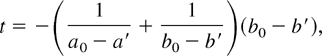
that ρ(t,x31,z) =
1, T1 has no direct impact on
T2 and the duration processes become conditionally
independent. In this situation identification essentially follows along
the lines of Heckman and Honoré (1989,
1990). We impose the natural restriction that
ρ(0,x3,z) = 1 so that the marginal
distributions with this model are also as in the conditionally independent
model.
We let K1(u1) =
K(u1,1),
K2(u2) =
K(1,u2), denote the marginal distribution
functions and indicate their derivatives by
Kj′, j = 1,2. The partial
derivatives of K are indicated by
K(j), j = 1,2. Note that
Kj(0) = 0 and
Kj(1) = 1, j = 1,2.
Assumption 5. For j = 1,2 Kj′
is left continuous at 1 and Kj′(1) =
Lj > 0.
Assumption 5 guarantees that a certain limiting ratio of the
Kj′'s in the proofs that follow
is well defined. Alternatively, one could allow for the
Kj′'s to vanish, by, say,
strengthening the smoothness assumption and using
L'Hôpital's rule.
PROPOSITION 1. Let Assumptions 1–5 hold. Then,
θj, Φj, j = 1,2,
ρ, and K are identifiable.
Proof. The survivor function of the minimum of the two durations is
given by
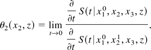
We can identify θ2 by evaluating the ratio
and observing that
We can identify θ1 symmetrically. To identify
K note that
By varying θ1 and θ2 over
,
we can trace out K. Because K is identifiable and
increasing in its arguments, K2 has a unique and
identifiable inverse, H2, such that
so that
and
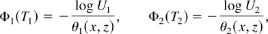
The term Φ1 is identified symmetrically. █
Remark 1. Without the identifying variable, x3, it
is still possible to identify the parameters using functional form
restrictions. Note that in this case we can identify
In general, it is not possible to decompose the left-hand side into
the two functions. However, for certain, fairly rich parametric models
one can show that, if ρ(t) = ρ(t;a)
and Φ(t) = Φ(t;b), where the true
values are a0 and b0, say, then
for any other values, a′ and b′, say,
ρ(t;a0) ≠
ρ(t;a′) and
Φ(t;b0) ≠
Φ(t;b′) on a set of positive measure.
Consequently, it is possible to identify the two functions.
For example, suppose Φ(t) =
ta, ρ(t) = (1 +
t)b and say for two values
a0,b0 and
a′,b′ these are the same. Then
or
a constant, which can only hold on a set of measure zero. The rest of
the identification follows as previously.
3. IDENTIFICATION WITHOUT EXCLUSION
RESTRICTIONS
In many situations it may not be plausible to impose exclusion
restrictions. For example, in bargaining situations, if both agents
have access to the same information, there is no reason to expect that
one agent will condition on less information than the other. However,
it may be plausible to make an assumption as to how a covariate will
impact on each agent's duration dependence, at least in a limiting
sense. In this case the data are generated as
where x (a scalar) and z, taking values on
,
are common to both θ1 and θ2. The
durations respond asymmetrically to x such that for, say, large
(small) values of x, we have θ1 → 0
(θ2 → 0) and we can assume that an observed exit is
due to T2 (T1) being the minimum.
It should be intuitive how the model is identified. The terms
Φ2 and θ2 are identified using values of
x such that, say, x ≥ x10.
Conversely, Φ1 and θ1 are identified using
values of x such that, say, x ≤ x20
(x20 < x10). We require that
the relevant normalizations can be imposed within these ranges. The
assumptions are as follows.
Assumption 6. The durations are generated as in equation (15) where
(U1,U2) ∼ K :
(0,1) × (0,1) → [0,1] ,
K(·,·) is strictly increasing and differentiable
in its arguments.
Assumption 7. θ(x,z) =
(θ1(x,z),θ2(x,z))
→ R+2 is continuous;
.
Assumption 8. For all
such that x > x10,
θ1(x,z) = 0 and for all
such that x < x20,
θ2(x,z) = 0, some
x10 > x20. For some
;
for some
.
PROPOSITION 2. Let Assumptions 2 and 5–8 hold. Then
Φj, j = 1,2 and K are identifiable,
θ1 is identifiable for x <
x20, and θ2 is identifiable
for x > x10.
Proof. Note first that for values of x such that x
> x10
so that
We identify θ1(x,z) symmetrically.
Setting t = 1 we can identify K by varying
θ1 and θ2 over
.
As in the proof of Proposition 1, we can then identify
Φj by inverting Kj,
j = 1,2. █
Remark 2. Note that Proposition 2 only partially identifies the model
(at least nonparametrically). Without imposing other restrictions we can
identify
θ1(x,z)(θ2(x,z))
only for those values of x,z such that x
< x20 (x >
x10).
Remark 3. The presence of z in θ1 and
θ2 allows us to vary these functions over
and identify K. Without z we would only be able to
observe θ1 and θ2 over, say,
(x20,∞) × (x10,∞),
so that K and Φj,j = 1,2, are
only partially identifiable. This problem can be partially circumvented by
assuming θ1, θ2 are differentiable. An
explanation is in the working paper version of this paper (Paric and Rilstone, 1999).
4. CONCLUSION
This paper has shown that, under a variety of restrictions, a class
of latent competing risks models can be identified. Because the
functions we consider are identified in terms of the observed durations
and their derivatives, our results suggest a couple of estimation
strategies. One possibility would be to use nonparametric analogs of
the survivor function and its derivatives. There are both theoretical
and practical difficulties involved with this, because the estimation
would involve calculations at boundary points. Alternatively, one could
parameterize the components of the model and use standard maximum
likelihood procedures. Simulation and empirical results in Paric and
Rilstone (1998, 2000) indicate that this works quite well.
The identification results in the paper can be readily extended to a
number of other econometric models. In the case of sample selection
problems one often observes the minimum or maximum of two or more
random variables. The prototype of this is the Roy (1951) model where one observes the maximum of, say,
salary offers. The framework of this paper is readily adaptable to that
model. Moreover, it is quite intuitive that the results would be useful
in the Roy context if an agent conditions on a sequence of wage offers.
The same analysis applies to auction models.
The latent feature of the data that is central to our paper is also
present in disequilibrium models of supply and demand where one
observes the minimum of these two functions but does not know which has
been observed. A number of examples are given in Maddala (1986). Our results are directly applicable with a
simple reinterpretation of the variables and functions in the model.
Another extension of the results of this paper would be for an
intermediate situation along the lines of Lee and Porter (1984) in which the “cause of failure”
is imperfectly observed. In this case, additional observables would be
DY and Y, say, where D indicates which
process was the minimum and Y equals one if D is
observed, zero otherwise, and possibly depends on the covariates.
Because Y is observable, its distribution is identifiable. The
complete observations could be used to identify the distribution of the
rest of the process.