2.1 Dispersion in one-dimensional, zero-mean, stationary and homogeneous turbulence

Considering dispersion of fluid particles in a one-dimensional, zero-mean, stationary and homogeneous turbulent velocity field, Taylor (Reference Taylor1922) expressed the variance of the particle displacement $X$ as

where $t$ is the travel time of the particle, $\langle v^{2}\rangle$ is the velocity variance and $R({\it\xi})$ is the velocity autocorrelation coefficient, both in a Lagrangian frame of reference.

Taylor also identified two regimes for which simple estimates of the mean squared particle displacement can be derived: one in which the travel time $t$ of the particle is sufficiently small for the correlation coefficient to be nearly unity, and another in which the travel time is much larger than the time it takes the autocorrelation coefficient to approach zero. Defining the Lagrangian integral time scale as $\mathscr{T}=\int _{0}^{t}R({\it\xi})\,\text{d}{\it\xi}$ , one may then derive the following asymptotic expressions

By differentiating these expressions one can obtain the corresponding rates of particle dispersion in the two regimes as

As equations (2.4) and (2.5) demonstrate, the rate of scalar dispersion would initially have a linear ballistic range, in which it would depend exclusively on the variance of the Lagrangian velocity fluctuations, followed by an intermediate range, which leads to a long-time range, in which the rate of dispersion would be independent of time and would depend on both the variance of the Lagrangian velocity fluctuations and the Lagrangian integral time scale of the turbulent field. The product $D=\langle v^{2}\rangle \mathscr{T}$ of the latter two quantities is known as the turbulent diffusivity, which in the following will also be referred to as the Taylor diffusivity.

2.2 Growth of a plume in homogeneous turbulence

Taylor’s dispersion theory may be adapted for the study of turbulent diffusion of a passive scalar injected from a line source in stationary and homogeneous turbulence that is convected by a mean stream. Consider a flow in which $x_{1}$ is the streamwise direction, $x_{3}$ is the ‘spanwise’ direction parallel to the axis of the source and $x_{2}$ is the ‘transverse’ direction normal to the two others. As usual, overlines will denote time averages, primes will denote standard deviations and one may consider diffusion in a frame convected with the mean speed $\overline{U}_{1}$ to estimate the diffusion time as $t\approx (x_{1}-x_{1s})/\overline{U}_{1}\equiv {\rm\Delta}x_{1}/\overline{U}_{1}$ , where $x_{1s}$ is the streamwise distance between the source and the arbitrary origin of the coordinate system and ${\rm\Delta}x_{1}$ is the streamwise distance from the source. Ensemble averages may be replaced by time averages, Lagrangian velocity variances may be approximated by Eulerian ones (Corrsin Reference Corrsin1975), the Lagrangian integral time scale may be estimated as $\mathscr{T}\approx L_{22,2}/u_{2}^{\prime }$ and the Taylor diffusivity may be approximated as

where $L_{22,2}$ is the integral length scale of transverse velocity fluctuations separated along the transverse direction.

One may then also transform Taylor’s dispersion estimates to the following expressions for the plume half-width in an Eulerian frame of reference

A more meaningful specification of the ranges of validity of the two asymptotic expressions for ${\it\sigma}$ would be in terms of the relative width of the plume in comparison to the size of the dominant turbulent eddies, rather than distance from the source. This can be easily achieved by solving the corresponding diffusion expressions for $x_{1}$ and rearranging the terms in the two inequalities. The result is

Using (2.8) (or, equivalently, (2.10)), one may estimate the Taylor diffusivity from the rate of plume growth, in the form of the so-called apparent turbulent diffusivity

In the previous description, we have not considered the very early stage of plume development, during which the size of the plume is extremely small and its spreading is due to molecular diffusion alone; this range has been termed as the molecular–diffusive range (Anand & Pope Reference Anand, Pope, Bradbury, Durst, Launder, Schmidt and Whitelaw1985). As the thermal plume grows, but still remains significantly narrower than the integral length scale of the turbulence, it is the amplitude of the transverse velocity fluctuations that dictates its growth rate; this region is known as the turbulent–convective range. Eventually, when the thermal plume width becomes sufficiently larger than the integral length scale of the flow, its growth rate is dictated by the variance of the transverse velocity fluctuations and the magnitude of the integral length scale; this range is known as the turbulent-diffusive range.

3.1 Experimental facility

Measurements of the scalar and turbulent velocity field were taken in an open circuit, blowing wind tunnel that had a 16:1 contraction and a test section with a height $h=0.305$  m, a nominal width of $1.5h$ and a working length of approximately $16.6h$ . All measurements were taken at a fixed inlet velocity of $U_{\infty }=10~\text{m}~\text{s}^{-1}$ , which was calculated from the measured pressure difference across the wind tunnel contraction; this speed was maintained constant by controlling the fan speed through an electronic feedback loop. The background turbulence levels were found to be $0.1\,\%$ in the streamwise direction and $0.2\,\%$ in the transverse direction at an inlet velocity of $U_{\infty }=10~\text{m}~\text{s}^{-1}$ . The test section was equipped with four insertion ports (‘slots’) for the insertion of the turbulence-generating grid and the heated line source, which was used to generated the scalar field. The first of these slots was located at a distance of $2.5h$ from the start of the test section, with the next three slots located at distances of $1h$ , $1.5h$ and $2h$ from the first slot, as shown in figure 1. The upstream part of the test section, up to the farthest downstream slot, had parallel walls, whereas the remainder had vertical walls that diverged slightly in order to compensate roughly for boundary layer growth along the four walls and so reduce the variation of the mean velocity in the core of the test section.

Figure 1. Scaled drawing of the wind tunnel used for the measurements. In the configuration shown here, a turbulence-generating grid was inserted in Slot A and the heated line source was placed in Slot B, but experiments were also conducted with the grid and the source inserted in different slots. In all cases, the origin of the coordinate system was located at the centre of the grid and $x_{1},x_{2},x_{3}$ were, respectively, the streamwise, transverse and spanwise axes. The distance from the turbulence grid to the heated line source, marked in this figure for one representative case, was denoted as $x_{1s}$ and could be positive or negative.

Figure 2. Scaled drawings of the turbulence-generating grids. Note that the origin of the coordinate system is the centre of the grid. (a) FSG, (b) RG160, (c) RG80, (d) RG18.

The turbulent field for each test was generated using one of the four planar grids shown in figure 2. All grids were machined from US 16 gauge sheets of metal (steel for the regular grids and, for higher strength, titanium for the fractal grid) with a standard thickness of 1.59 mm and having the specifications listed in table 1. It is well known from the literature that, for a given grid design, the turbulence characteristics depend mainly on the solidity (namely, the ratio between the solid cross-sectional area of the grid and the cross-sectional area of the test section) and the mesh size (namely, the spacing between the elements) of the grid; the cross-sectional shape of grid elements, their thickness in the direction of the flow and the separation of their centreplanes, if present (e.g. for biplanar square grids), also play a role, as they influence the grid’s ‘effective’ solidity. When comparing the performances of grids of different designs, it is not immediately apparent which parameters should be matched. To begin with, the dimensions of our wind tunnel cross-section imposed an upper bound for the mesh size of a regular grid and the spacing of the largest elements of the fractal grid. Consequently, we constructed grids of both designs with corresponding spacings that were as large as possible for these devices to qualify as grids and not to consist of isolated elements; it goes without saying that the two spacings were matched. We expected that each of these two grids would produce the strongest possible turbulence by comparison to smaller grids with similar geometrical features. We further conjectured that, for a meaningful comparison of the performance of grids of different sizes, and even different designs, one must also match their solidities, as this would ensure that the pressure drop behind all grids would be roughly the same; we note that this is true not only for regular grids, but also for fractal square grids (Laizet & Vassilicos Reference Laizet and Vassilicos2015). The solidity of all our grids was set to $0.25\pm 0.02$ , in line with values used in previous studies of fractal grids. Finally, to minimise element thickness effects, we machined all grids from metallic sheets of the same standard thickness, which was actually chosen to be the smallest one that would ensure their structural integrity. One of the grids (‘fractal square grid’ – FSG) was multiscale, which is a geometry known to produce extended downstream regions of $C_{{\it\varepsilon}}\neq$ constant. This grid, which had $N=4$ levels of partially overlapping elements, was made of titanium to ensure sufficient stiffness of the smallest elements and was sanded following machining to remove edge roughness. The length and the frontal thickness of the largest elements in FSG were, respectively, indicated as $L_{0}$ and $t_{0}$ , and those of subsequent levels as $L_{1},t_{1}$ etc. FSG was designed such that the thickness ratio, $t_{r}$ , between the largest and smallest bars was $t_{r}=t_{0}/t_{3}=22.3$ . Consequently, the ratio between subsequent elements were determined as $R_{t}=t_{r}^{1/(1-N)}=0.355$ . As with previous fractal grid designs (Valente & Vassilicos Reference Valente and Vassilicos2011, Reference Valente and Vassilicos2012; Gomes-Fernandes, Ganapathisubramani & Vassilicos Reference Gomes-Fernandes, Ganapathisubramani and Vassilicos2012; Hearst & Lavoie Reference Hearst and Lavoie2014; Valente & Vassilicos Reference Valente and Vassilicos2014, Reference Valente and Vassilicos2015), the ratio between the length of subsequent elements was set to 0.5; as an example, $L_{1}=0.5L_{0}$ . The three other grids (RG160, RG80 and RG18) were ‘regular’ square grids, each with elements closely matching the first-, second- and fourth-level elements of FSG. RG18 also matched the effective mesh size (Hurst & Vassilicos Reference Hurst and Vassilicos2007) of FSG.

Based on previous literature of FSG (Valente & Vassilicos Reference Valente and Vassilicos2011, Reference Valente and Vassilicos2012; Gomes-Fernandes et al. Reference Gomes-Fernandes, Ganapathisubramani and Vassilicos2012; Hearst & Lavoie Reference Hearst and Lavoie2014; Valente & Vassilicos Reference Valente and Vassilicos2014, Reference Valente and Vassilicos2015) one would expect to observe $C_{{\it\varepsilon}}\neq$ constant for downstream distances of less than $2x_{\ast }$ , where $x_{\ast }=L_{0}^{2}/t_{0}$ is the wake interaction length scale for the largest elements (Mazellier & Vassilicos Reference Mazellier and Vassilicos2010). A recent study by Valente & Vassilicos (Reference Valente and Vassilicos2014) showed that regular grids would also produce regions of the flow in which $C_{{\it\varepsilon}}\neq$ constant. As a possible indicator of such regions, we have listed the corresponding values of $x_{\ast }$ in table 1.

The passive scalar field was generated by electrically heating a thin ribbon made of Nichrome alloy (toaster element) and stretched horizontally across the width of the tunnel. The ribbon was kept taut while at a high temperature by having one of its ends fixed to its wooden frame and the other end spring mounted, with the tension adjusted by turning two nuts along a threaded bar. The heating ribbon had a frontal thickness of 0.13 mm and a streamwise width of 1.59 mm and supplied with a constant power of 180 W. In this article, we present tests with the heat source inserted at four different slots, two of which were downstream of the turbulence-generating grid, one was upstream of the grid and one was on the same slot as the grid. As shown for a representative case in figure 1, the distance between the source and the grid is denoted as $x_{1s}$ . For convenience, these tests will be referred to as HS1 (for the $x_{1s}=h$ case), HS2.5 (for the $x_{1s}=2.5h$ case), HS–1 (for the $x_{1s}=-h$ case) and HS0 (for the $x_{1s}\approx 0$ case; to be precise, $x_{1s}=-0.02h$ ). The locations of grid insertion slots in our wind tunnel fortuitously permitted us to introduce the scalar at two structurally distinct regions of grid turbulence: as shall be shown in § 4.2, the HS2.5 cases correspond to decaying turbulence fields for all the grids, whereas the HS1 cases correspond to the ‘production regions’ of the turbulence fields (i.e. where the turbulence intensity increases with streamwise distance) for FSG, RG160 and RG80. In summary, the present four choices of source locations are expected to enable us to obviate the effects of turbulence history on the diffusion of the thermal plume.

3.2 Instrumentation

The streamwise and transverse velocity components were measured simultaneously with a cross-wire probe having sensors made of tungsten with a diameter of $2.5~{\rm\mu}\text{m}$ , sensing length of 0.85 mm and a distance between sensors of 0.5 mm. Therefore, the sensor length-to-diameter ratio was 340, which is deemed to be sufficiently large for conduction effects to be negligible (Li et al. Reference Li, Mckeon, Jiang, Morrison and Smits2004). The probe was operated with AALabs1004 Constant Temperature Anemometers. The signals were low pass filtered by analogue filters with cutoff frequencies of 14 kHz, digitised at a rate of 30 kHz and recorded over 60 s for each test. The cross-wire probe was calibrated in situ using a velocity-pitch-map calibration method, also referred to as look-up table calibration (Lueptow, Breuer & Haritonidis Reference Lueptow, Breuer and Haritonidis1988). Measurements were taken along the centreline ( $x_{2}=0,x_{3}=0$ ) for downstream distances of $h\leqslant x_{1}\leqslant 12h$ in $0.25h$ increments. Transverse profiles, ranging between $-h/3\leqslant x_{2}\leqslant h/3$ , were also measured at selected downstream distances. All measurements were acquired with an inlet velocity of $U_{\infty }=10~\text{m}~\text{s}^{-1}$ , so that the large element Reynolds numbers for FSG, RG160, RG80 and RG18 were, respectively, $Re_{L_{0}}=U_{\infty }L_{0}/{\it\nu}\approx 104\,000,102\,000,51\,000$ and 11 500.

The local mean flow temperature was measured with a glass-coated thermistor probe (EPCOS(TDK), B57540 series, manufacturer part number: B57540G1103F, 10  $k{\it\Omega}$ 1 % RAD). The thermistor was connected to a homemade circuit that provided a low excitation current of $50~{\rm\mu}\text{A}$ ; the self-heating of the thermistor was estimated to raise its temperature by $0.06\,^{\circ }\text{C}$ . Temperature fluctuations were measured with a cold-wire probe, having a sensor made of platinum with a diameter of $1~{\rm\mu}\text{m}$ and a length-to-diameter ratio of 500. The sensor was etched from Wollaston wire and spot welded onto a DANTEC 55P31 temperature probe tip, which was then plugged into a DANTEC 55H21 probe holder. The cold wire was operated at a constant current of 0.3 mA, provided by a low noise and high gain homemade circuit. The thermistor and cold-wire probes were positioned at the same streamwise and transverse positions and were separated by 5 mm in the spanwise direction. The two signals were sampled simultaneously at a rate of 20 kHz for 30 or 60 s, depending on the heating configuration. The signal from the cold wire was passed through an 8 kHz analogue low pass filter before being digitised. The flow temperature upstream of the heated source was monitored with a precalibrated 100 ${\it\Omega}$ resistance temperature detector (29348-T01-B-48, RDF Corp.); this temperature was subtracted from the downstream flow temperature to account for room temperature variation. Temperature measurements were taken in the vertical plane of the wind tunnel at the same downstream positions as the turbulence measurements, but the two sets of measurements were made at different times. All data were digitised using a 16-bit data acquisition system (national instruments, PCI 6143).

3.3 The measurement of turbulence properties

The turbulent kinetic energy parameter $k$ was estimated as $k\approx 0.5\overline{u_{1}^{2}}+\overline{u_{2}^{2}}$ , under the assumption that the turbulence was axisymmetric, which is fair for grid turbulence (Comte-Bellot & Corrsin Reference Comte-Bellot and Corrsin1966; Nagata et al. Reference Nagata, Sakai, Inaba, Suzuki, Terashima and Suzuki2013). The streamwise integral time scale $T_{11}$ was determined by integrating the temporal autocorrelation coefficient of the streamwise velocity fluctuations to its first zero; then the streamwise integral length scale was estimated as $L_{11,1}\approx T_{11}\overline{U}_{1}$ . The streamwise Taylor microscale ${\it\lambda}$ was determined with the use of Taylor’s frozen flow approximation as

the turbulent Taylor Reynolds number was calculated from (1.2) and the rate of kinetic energy dissipation per unit mass was estimated as

Possible measurement errors introduced by the limited spatial resolution of the cross-wire were estimated using procedures suggested by Burattini (Reference Burattini2008). It was found that such errors in the measured Reynolds stresses and integral length scales would be at most of the order of 1 %, which are deemed to be negligible and part of the overall measurement uncertainty. On the other hand, parameters calculated from measurements of the streamwise velocity derivative were subjected to appreciable biases: ${\it\lambda}$ and $Re_{{\it\lambda}}$ appeared to be underestimated by approximately 12 %–2 % along the measurement section, whereas ${\it\varepsilon}$ and $C_{{\it\varepsilon}}$ appeared to be overestimated by approximately 22 %–4 % in the same range. These biases were removed in the reported results by applying appropriate corrections. It is noted, however, that the corrections proposed by Burattini (Reference Burattini2008) were meant to apply to decaying homogeneous and isotropic turbulence, which, as shall be shown in the following section, is not the case in the regions close to our grids. Nevertheless, we considered that application of these corrections removed a major portion of the bias and absorbed any remaining (positive or negative) bias into the overall measurement uncertainty, which includes precision uncertainty and the effects of imperfect match of theoretical and experimental conditions. In any case, as will be discussed later, our main conclusions are not affected by small errors in velocity derivatives.

4.1 The mean flow fields and transverse turbulence inhomogeneity levels

The streamwise variation of the centreline mean velocity, normalised by the inlet velocity, is shown in figure 3 for the four grid configurations. In all cases (if one employs a plausible extrapolation of the RG18 data towards the grid) this ratio exceeded unity in a range close to each grid and then decreased, eventually settling to near-unity values further downstream. For the three sets of results that extended to that location, slight kinks may be observed at approximately $x_{1}/h=4.5$ , where wall divergence commenced. The far downstream level of $\overline{U}_{1}/U_{\infty }$ was somewhat smaller than unity for FSG and RG160 and somewhat larger than unity for RG80 and RG18. This difference is compatible with the expectation that the boundary layers would be thinner for the larger grids, as the result of more thorough mixing with core flow transported by large eddies. In the region near each grid, the local mean velocity was significantly larger than $U_{\infty }$ ; this may be confidently attributed to the fact that the wind tunnel centreline passed through unobstructed regions of all grids, which would have jet-like velocity profiles.

Figure 3. Measurements of the dimensionless mean velocity along the centreline of the wind tunnel downstream of the four grids (connected by solid lines); the maximum (open symbols) and minimum (closed symbols) normalised velocities on selected transverse planes are also shown.

In figure 3, we also show the maximum and minimum normalised mean velocities on selected transverse planes. These results show that, for all grids, the mean velocity became essentially uniform for $4.5\leqslant x_{1}/h$ . A more complete analysis of the homogeneity level of the velocity field is given in figure 4, which shows transverse profiles of the mean velocity, the standard deviation of the transverse velocity fluctuations and the streamwise integral length scale downstream of the four grids. Values at each downstream location were normalised with the corresponding local centreline value in order to obviate the local level of transverse non-uniformity. At the two closest downstream locations, there were clear signs of mean flow non-uniformity for FSG, RG160 and RG80, but these became negligible further downstream. All measured mean flow profiles downstream of the RG18 were essentially uniform. The turbulence behind FSG, RG160 and RG80 was clearly transversely inhomogeneous at $x_{1}/h=1.00$ , but the inhomogeneity was reduced to negligible levels further downstream.

Figure 4. Transverse profiles of the streamwise mean velocity (a), standard deviation of the transverse turbulent velocity (b) and streamwise integral length scale (c), all normalised with the corresponding local centreline values; measurements downstream of the four grids are marked using the symbols shown in table 1 with increasing darkness for the three larger grids at $x_{1}/h=1.00,2.50,4.50,5.75,7.00$ and $8.50$ , but for RG18 only at $x_{1}/h=1.00,2.50$ and $4.50$ .

4.2 The evolution of turbulence properties

Figure 5. Streamwise evolution of turbulence properties downstream of FSG (a) and RG160 (b). Crosses denote measured values before the application of corrections; cases with indistinguishable corrected and uncorrected values are not differentiated in these plots.

Figure 6. Streamwise evolution of turbulence properties downstream of RG80 (a) and RG18 (b). Crosses denote measured values before the application of corrections; cases with indistinguishable corrected and uncorrected values are not differentiated in these plots.

Figures 5 and 6 present the evolution of pertinent turbulence properties along the centreline downstream of the four grids. An important point to keep in mind when comparing the results is that, unlike those used by previous investigators, all of our grids had the same solidity. Another general note is that because the near field of RG18 was not of much interest in this work, our measurements for this grid did not include the ‘production region’, where the turbulence was generated and which would extend to a much shorter downstream distance than the production regions of the three larger grids. For brevity, we will exclude this grid from some of the following discussion; nevertheless, all available evidence indicates that its turbulence, when properly scaled, follows the same trends as those downstream of the two other regular grids.

For the three larger grids, $u_{1}^{\prime }$ (as well as $u_{2}^{\prime }$ , not shown in the figure) presented a distinct peak at a downstream distance $x_{peak}$ that was smallest for RG80, intermediate for FSG and largest for RG160. When normalised by the wake interaction length scale $x_{\ast }$ , the peak distances were $x_{peak}/x_{\ast }\approx 0.63$ for the two regular grids and $0.35$ for the fractal grid. These values are generally consistent with the available literature. Valente & Vassilicos (Reference Valente and Vassilicos2012) also reported values $x_{peak}\approx 0.63x_{\ast }$ for two square grids with solidity 0.17 and mesh sizes of 230 and 115 mm. Moreover, Mazellier & Vassilicos (Reference Mazellier and Vassilicos2010) reported $x_{peak}\approx 0.45x_{\ast }$ for their SFG17 square fractal grid, which had a solidity of 0.25, a thickness ratio of $t_{r}=17$ and a length of the largest bar $L_{0}=237.8$ mm, as well as three other fractal grids, all of which had the same solidity but smaller thickness ratios; it is noted, however, that more recent measurements for the same SFG17 grid by Laizet, Nedić & Vassilicos (Reference Laizet, Nedić and Vassilicos2015) have shown the peak to be at $x_{peak}\approx 0.41x_{\ast }$ . The observed small differences in peak location for the fractal grids in the present and previous studies may be attributed to differences in grid design.

In all cases, and throughout the measurement range, the anisotropy ratio $u_{1}^{\prime }/u_{2}^{\prime }$ was greater than unity, in agreement with the vast literature on grid turbulence. This ratio first reached a peak at some distance from the grid and then decreased gradually towards values in the vicinity of 1.25, in conformity with previous studies using similar grids (Valente & Vassilicos Reference Valente and Vassilicos2011; Gomes-Fernandes et al. Reference Gomes-Fernandes, Ganapathisubramani and Vassilicos2012; Hearst & Lavoie Reference Hearst and Lavoie2014); for RG18, the anisotropy ratio tended towards values much closer to unity, which is attributed to fact that the turbulence produced by this grid decayed much faster than in the other cases.

It is interesting to note that the locations of the peaks of $u_{1}^{\prime }$ and $u_{1}^{\prime }/u_{2}^{\prime }$ coincided for each of the three larger grids; these locations may be used to divide each flow field into an upstream region, where the effects of the grid elements dominated the turbulence structure, and a downstream region, where the mean shear was negligible, the turbulence was nearly transversely homogeneous and isotropic and the turbulent kinetic energy decayed. It is the latter region, to be referred to hereafter as ‘decaying grid turbulence’ (DGT), which is of main interest in this work. The streamwise evolution of $Re_{{\it\lambda}}$ , also shown in figures 5 and 6, demonstrates that this property also had a peak, whose location coincided with the peak location for $u_{1}^{\prime }$ for each of the three larger grids, and then decreased monotonically in the DGT region. This behaviour is well known for grid turbulence, but is noted here as it implies that the function $Re_{{\it\lambda}}(x_{1})$ would be single valued only if DGT were considered in isolation from the upstream region. This is an important reason to focus on DGT when investigating the possible dependence of $C_{{\it\varepsilon}}$ on $Re_{{\it\lambda}}$ .

Now, let us compare the magnitudes of some relevant turbulence characteristics behind the four grids at a fixed downstream location in the DGT region. The ranking of the grids was always in the order R160, FSG, RG80 and RG18, irrespective of which parameter was used for such comparison and which location was selected. This ranking corresponds to decreasing $u_{1}^{\prime }$ (and $k$ ), $Re_{{\it\lambda}}$ and $L_{11,1}$ and increasing ${\it\lambda}/L_{11,1}$ and ${\it\eta}/L_{11,1}$ . This order is not surprising when considering the three regular grids, as it is well known that the previous parameters are monotonic functions of the mesh size. However, the observation of the performance of FSG relative to RG160 is rather novel, as the literature contains no specific studies of turbulence generated by regular and fractal grids with the same solidity and $L_{0}$ . One exception is the study by Laizet et al. (Reference Laizet, Nedić and Vassilicos2015), in which one of the fractal square grids had comparable $L_{0}$ and solidity to a grid composed solely of the central square element of the fractal square grid. This study, however, presented no comparisons between the streamwise evolution of the turbulence behind the two grids, as its main focus was the behaviour of the energy spectrum.

The bottom panels in figures 5 and 6 show the streamwise evolution of the dissipation parameter $C_{{\it\varepsilon}}$ . It is evident that $C_{{\it\varepsilon}}\approx \text{const.}$ in substantial regions of all panels, which extended over the furthest downstream part of the corresponding DGT region. We shall refer to the $C_{{\it\varepsilon}}\approx \text{const.}$ region as the ‘fully developed region’ (FDR), as it is the region in which not only $k$ and ${\it\varepsilon}$ , but also $L_{11,1}$ evolved in consistent and self-similar manners, which rendered the dissipation parameter constant. The values of $C_{{\it\varepsilon}}$ in the FDR were 1.4 for FSG and RG160, 1.7 for RG80 and 2.0 for RG18. It is noted that our definition of this parameter and those of the turbulent kinetic energy, dissipation rate, integral length scale and microscale differ from definitions used by previous researchers; when we applied the same definitions, we obtained estimates of $C_{{\it\varepsilon}}$ in the FDR that were close to values in the literature (Valente & Vassilicos Reference Valente and Vassilicos2012; Hearst & Lavoie Reference Hearst and Lavoie2014). The upstream boundary of the FDR was in the range $1.3\lesssim x_{1}/x_{\ast }\lesssim 3$ , depending on the grid, in conformity with previous findings (Valente & Vassilicos Reference Valente and Vassilicos2012; Isaza, Salazar & Warhaft Reference Isaza, Salazar and Warhaft2014). Upstream of the FDR, but still within the DGT region, $C_{{\it\varepsilon}}$ grew monotonically with increasing streamwise distance, while $Re_{{\it\lambda}}$ decreased monotonically. This observation points to a possible inverse relationship between these two parameters. For the three larger grids, we could fit the data quite well with power laws of the type $C_{{\it\varepsilon}}\propto Re_{{\it\lambda}}^{-1}$ in a substantial upstream subregion of DGT. We shall refer to this subregion by the term ‘developing region’ (DR), under the postulate that it contained turbulence whose structure gradually developed towards the scaling found in the FDR. Regions of grid turbulence described by this power law have been recently discovered by several previous investigators (see review by Vassilicos (Reference Vassilicos2015)); the state of the flow in such regions has been referred to by the name ‘non-equilibrium turbulence dissipation law’. Besides the fact that equilibrium turbulence, in the manner described by Vassilicos (Reference Vassilicos2015), may be unachievable behind grids and so all grid turbulence may be viewed to be in non-equilibrium, the restriction of the term ‘non-equilibrium’ to this specific power law would not permit its use to other flows, or even other subregions of grid turbulence, in which a power law with an exponent that is different from $-1$ may be found to hold (see our recent study of uniformly sheared flows (Nedić & Tavoularis Reference Nedić and Tavoularis2016)). For these reasons, we chose to introduce the term ‘developing region’ for the initial part of decaying grid turbulence, where $C_{{\it\varepsilon}}\propto Re_{{\it\lambda}}^{-1}$ .

Of course, there is also a subregion between the DR and the FDR, in which smooth transition was achieved from the DR expression for $C_{{\it\varepsilon}}$ to the one in FDR; we shall refer to this as ‘partially developed region’ (PDR). This subregion was significantly wider for FSG than for RG160 and RG80, presumably because the turbulence structure behind FSG was more complex. Although not attaching much significance to this finding, as it is not central to the present objectives, we found that, for the FSG, RG160 and RG80 cases, the data in much of the PDR could be approximately fitted with the power law $C_{{\it\varepsilon}}\propto Re_{{\it\lambda}}^{-0.6}$ .

Note that figures 5 and 6 present both corrected and uncorrected values of $Re_{{\it\lambda}}$ and $C_{{\it\varepsilon}}$ . Despite the significance of corrections in the developing region, the observation that $C_{{\it\varepsilon}}\propto Re_{{\it\lambda}}^{-1}$ applies equally well to both the corrected and uncorrected results.

4.3 Turbulence decay rates

The decay of turbulent kinetic energy generated by grids and similar regularly spaced obstructions with a spacing $L_{0}$ has been conventionally described by a power law of the normalised streamwise distance from an effective origin $x_{10}$ , namely as

Despite considerable effort over many decades to devise a theoretical justification for this relationship, it remains empirical and the parameters $a$ , $x_{10}$ and $m$ are determined by curve fitting to measurements. Previously determined values of the exponent $m$ for data in the fully developed region of decaying grid turbulence (FDR-DGT), typically between 1.1 and 1.4 (Comte-Bellot & Corrsin Reference Comte-Bellot and Corrsin1966; Gad-el Hak & Corrsin Reference Gad-el Hak and Corrsin1974; Mohamed & LaRue Reference Mohamed and Larue1990; Lavoie, Djenidi & Antonia Reference Lavoie, Djenidi and Antonia2007; Sinhuber, Bodenschatz & Bewley Reference Sinhuber, Bodenschatz and Bewley2015) are lower than those in the developing region of decaying grid turbulence (DR-DGT), which are typically between 2.4 and 3.0 (Valente & Vassilicos Reference Valente and Vassilicos2011; Hearst & Lavoie Reference Hearst and Lavoie2014; Isaza et al. Reference Isaza, Salazar and Warhaft2014; Valente & Vassilicos Reference Valente and Vassilicos2015). When the ranges of measurements are relatively narrow, however, the sensitivity of curve fits to the value of $x_{10}$ may be high and so several combinations of parameter values may end up producing good fits. Indeed, this was the case for the present results and so we found that it would be more meaningful to adopt the same value of $x_{10}/L_{0}$ for each of the states of turbulence produced by all grids, rather than determining specific values of this parameter by low-sensitivity optimal fitting. In accordance with established sources, we chose the values $x_{10}/L_{0}=3.5$ for FDR-DGT (Comte-Bellot & Corrsin Reference Comte-Bellot and Corrsin1966) and $-3.5$ for DR-DGT (Valente & Vassilicos Reference Valente and Vassilicos2011).

Figure 7. Decay of the kinetic energy, normalised by $L_{0}$ (a) and $x_{\ast }$ (b), downstream of the grids. Circles, squares, triangles and stars denote data for, respectively, FSG, RG160, RG80 and RG18. Open symbols denote measurement points in the DR-DGT and closed symbols denote measurement points in the FDR-DGT. Solid lines are power functions fitted to the data with exponents as listed in table 2.

As shown in figure 7, all data in the ranges of both states produced by our grids were fitted well by power functions. The ranges used for fitting the data in the DR and the FDR, in terms of $x_{1}/x_{\ast }$ and $x_{1}/L_{0}$ , have been listed in table 2. The exponents of these functions, also listed in table 2, were within the ranges of values encountered in the literature for both FDR-DGT and DR-DGT. We have also fitted alternative power functions to the same data, under the assumption that their effective origins were on the grid, namely that $x_{10}=0$ ; these functions also fitted very well to all our data but their exponents, also listed in table 2, were significantly higher than the previous ones in FDR-DGT and lower in DR-DGT. These results also conform with the literature (Valente & Vassilicos Reference Valente and Vassilicos2011; Isaza et al. Reference Isaza, Salazar and Warhaft2014). We refrained from presenting power laws in the PDR, because their ranges were too narrow for meaningful fits and the fitted exponents were overly sensitive to the choice of effective origin. In the remainder of this article, we shall mainly focus on the DR and the FDR of DGT.

5.1 Measurements of plume growth

Figure 8. Transverse profiles of the normalised mean temperature for all grids and source locations. Data taken within the range $2.5\leqslant {\rm\Delta}x_{1}/h\leqslant 3.0$ ; a fitted Gaussian function is shown by a white dashed line.

Transverse profiles of the local mean temperature rise ${\rm\Delta}\overline{T}$ above the unheated flow temperature were measured at several locations downstream of all four grids and with the source located upstream of the grid (HS-1), at the grid (HS0) or downstream of the grid (HS1 and HS2.5). All profiles, irrespective of the grid used, location of the source and location of measurement, could be fitted well by Gaussian functions. In the following, the local mean temperature rise will be normalised by the corresponding centreline value ${\rm\Delta}\overline{T_{c}}$ and transverse distances in the plume will be normalised by the ‘standard deviation’ ${\it\sigma}$ of the fitted Gaussian function, to be referred to as the plume half-width. An assortment of representative measurements for all our grids and source locations, together with the Gaussian fit, are shown in figure 8. Several previous investigators (Uberoi & Corrsin Reference Uberoi and Corrsin1952; Townsend Reference Townsend1954; Warhaft Reference Warhaft1984) have also reported Gaussian passive scalar plumes downstream of line sources in grid turbulence, while plume Gaussianity is a common assumption of previous diffusion models (Stapountzis et al. Reference Stapountzis, Sawford, Hunt and Britter1986; Viswanathan & Pope Reference Viswanathan and Pope2008; Pope Reference Pope2011). The present results complement these studies, but also introduce a novel finding: the mean temperature profile was Gaussian not only in the FDR-DGT, but also in the DR-DGT in which $C_{{\it\varepsilon}}\propto Re_{{\it\lambda}}^{-1}$ , including locations where the mean velocity was non-uniform and the turbulence was transversely inhomogeneous. Based on this observation, we may postulate that passive scalar plume Gaussianity is robust and may persist even in mildly non-uniform mean velocity fields. Support for this postulate is also provided by the observed Gaussianity of scalar plumes in uniformly sheared turbulence (Karnik & Tavoularis Reference Karnik and Tavoularis1989) and in a channel flow (Lavertu & Mydlarski Reference Lavertu and Mydlarski2005).

The downstream evolution of the thermal plume half-width ${\it\sigma}$ for all examined cases are shown in figure 9. Because a main objective of this study is to identify conditions that lead to the widest possible plume spreading at a fixed streamwise location, both ${\it\sigma}$ and the streamwise distance from the source have been normalised by the test section height $h$ and not by grid-related scales; an additional benefit of this normalisation is that it would readily demonstrate a possible confinement of the plume by the test section walls.

Figure 9. Evolution of the thermal plume half-width ${\it\sigma}$ downstream of FSG, RG160, RG80 and RG18; (a) HS1; (b) HS2.5; (c) HS-1; (d) HS0. For all cases, error bars indicate the 95 % confidence level of Gaussian fitting to the transverse mean temperature profiles. Circles, squares, triangles and stars denote data for, respectively, FSG, RG160, RG80 and RG18.

If we first compare results downstream of the three regular grids, it becomes evident that, in general, plume spreading increased with increasing grid mesh size. This is hardly a surprise, as larger grids produced turbulence with both larger intensity and larger scale at downstream positions that were far enough from all grids for the corresponding flows to be fully turbulent. This, however, is not necessarily the case for the close-to-the-grid fields of sources located upstream of the grid. An example is the $(x_{1}-x_{1s})/h\leqslant 3$ range for the HS-1 case, where ${\it\sigma}$ for RG80 was larger than that for RG160; it is noted that, in the near field, RG80 generated turbulence that had a higher intensity than those produced by FSG or RG160, which resulted in a larger initial plume spreading. It should be noted that the RG160 mesh size was roughly equal to half the test section height. Consequently, over a considerable range of the HS-1 and HS0 measurements, plume spreading would be very sensitive to the transverse location of the source; in the present case, in which the source was along the centre plane of the grid and measurements were taken along a line passing through the (unobstructed) centre of the grid, scalar diffusion would be subjected to relatively low turbulence over a part of its shown history that was much more significant for RG160 than for the smaller grids. This effect was aggravated when the source was placed upstream of the grid (HS-1 and HS0 cases). As a note of precaution to future users, we would like to mention that, while attempting to position the source closely downstream of the grid (namely, within the recirculating parts of the wakes of the grid elements), we observed that sections of the heated ribbon were overheating, which indicated poor convective heat transfer; no such problem was encountered when the source was located closely upstream of the grid elements.

The next practical question that we addressed was to identify the position of the grid with respect to the source that would produce the largest plume spreading. While comparing the measurements for different grid positions, we excluded the plume region close to the source ( $(x_{1}-x_{1s})/h\lesssim 1$ ), where plume spreading would depend strongly on the transverse location of the source. As figure 10 shows for the RG160 case, for all plume positions examined, it was the HS1 case that produced the largest plume spreading at a given distance from the source. The observation that the HS1 plume was wider than the HS2.5 plume is consistent with the fact that, although the turbulence intensity at $x_{1}/h=1$ was lower than at 2.5, it increased to a peak intensity that was higher than at 2.5 before decaying, hence exposing the scalar to an overall more intense turbulence field. A similar, although more complex, logic may be employed to explain why the HS1 plume was wider than the HS0 plume; whereas the HS1 plume was exposed to strong turbulence from the start, spanwise sections of the HS0 plume were exposed to no turbulence in the initial phase of plume development, which essentially shifted the effective origin of the plume downstream. In summary, our results demonstrate that there is an optimum position of the grid relative to the plume source, which is likely to be somewhere around the HS1 location; we shall revisit this issue later in the paper.

Figure 10. Plume spreads at different distances from the source for four different positions of RG160 relative to the source; results have been normalised by the plume spread for HS1. Streamwise distances are, from light to dark symbols, $x_{1}-x_{1s}=2.5$ , 3.5, 4.5, 5.5, 6.5 and $7.5h$ .

Now, let us compare the results for RG160 and FSG, which had approximately the same values of $L_{0}$ and the same solidity. Figure 9 shows clearly that, when the source was placed downstream of the grid (HS1 and HS2.5), RG160 produced wider plumes from their start to the last measuring station. This was predictable on intuitive grounds, because the turbulence produced by RG160 in the measurement ranges was stronger than that produced by FSG in both intensity and length scale. With the source located upstream of the grid (HS-1 and HS0), the plume widths behind RG160 and FSG were indistinguishable for $(x_{1}-x_{1s})/h\leqslant 2.75$ for HS-1 and $(x_{1}-x_{1s})/h\leqslant 2$ for HS0. Further downstream, the plume spread more behind RG160 than behind FSG, in the same manner as for the downstream source locations. One might reasonably expect, however, that FSG would produce a marginally wider plume than RG160 in the near field, a postulate which is compatible with physical intuition concerning the effects of the second-, third- and fourth-level elements in FSG on the production of turbulence and the spreading of the plume. Whereas the plume along the centreline in the near field of RG160 spread mainly by molecular diffusion, the plume behind FSG was subjected to turbulent diffusion produced by the higher-level elements. As soon as the smaller-scale turbulence of higher-level elements, however, started interacting with the turbulence in the wakes of the first-order elements, it effectively broke down the largest eddies and so it contributed to the faster decay in the far field of FSG and the lower plume spreading rate. At first glance, the present findings appear to contradict a past assertion that the SSU mechanism, which is activated by fractal grids, generally enhances scalar diffusion (Suzuki et al. Reference Suzuki, Nagata, Sakai and Hayase2010a ,Reference Suzuki, Nagata, Sakai and Ukai b ; Laizet & Vassilicos Reference Laizet and Vassilicos2015). Nevertheless, a closer examination of the conditions in previous studies that led to this assertion proves that this is not the case. These studies, which include both experimental and numerical ones, found that scalar diffusion behind fractal grids was more efficient than diffusion behind regular grids with mesh sizes that were much smaller than the spacing $L_{0}$ of the largest elements of the fractal grids. This finding is identical to our own observation that FSG diffused the scalar more efficiently than RG18. Our investigation is the first to compare scalar diffusion and mixing behind a fractal grid and a regular grid with the same solidity and roughly the same mesh size as the largest fractal element spacing, which we believe to be a more appropriate comparison than those made in the past.

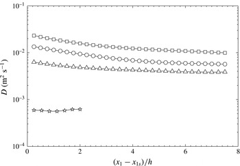
Figure 11. Streamwise variation of the Taylor diffusivity $D$ for all the grids for the HS2.5 case. Circles, squares, triangles and stars denote data for, respectively, FSG, RG160, RG80 and RG18.

Thus far, we have justified our observations on the intuitive notion that turbulent diffusion would generally be enhanced by increases in the turbulence intensity and the size of energy containing eddies. The product of these two parameters is essentially the (turbulent) Taylor diffusivity, which is a cornerstone of Taylor’s diffusion theory. It seems therefore worthwhile to investigate the degree by which this simplified theory, as outlined in § 2.2, may provide theoretical support for the present observations. Representative examples of the Taylor diffusivity are presented in figure 11 for the HS2.5 case, but it is noted that similar results for the other locations of the source would lead to the same qualitative observations. For this figure, the Taylor diffusivity was estimated as $D=u_{2}^{\prime }L_{11,1}/2$ , which introduces considerable uncertainty in view of a possible streamwise variation of the ratio $L_{22,2}/L_{11,1}$ . Nevertheless, it is clear that the Taylor diffusivity was largest for RG160, followed by FSG, RG80 and RG18, and so followed the same order as the spreading of the thermal plume.

In view of the results shown in figure 11, we may now revisit the search for an optimum position of the grid relative to the plume source. On intuitive grounds, we may argue that the widest plume at a given distance from the source would be the one that experienced the strongest turbulence cumulatively during its evolution. In other words, one would expect that the grid that produced the highest average Taylor diffusivity in the entire plume would also produce the largest spreading of the plume. To test this hypothesis, we define the average centreline Taylor diffusivity at a location that was $7.5h$ downstream of the source as

This average diffusivity is a function of the distance $x_{1s}$ between the grid and the source and it is reminded that the origin of the coordinate system was on the grid centreplane. To account for the transverse variation of the Taylor diffusivity, we may further define an average Taylor diffusivity in the core of the test section as

Figure 12. Streamwise variation of the average Taylor diffusivities along the centreline (solid line) and in the core of the test section (dashed line), for RG160 and a mixing length of 7.5 $h$ .

Figure 12 shows both average diffusivities for RG160 as functions of grid location in the range $1\leqslant x_{1s}/h\leqslant 2.5$ and a mixing length of 7.5 $h$ (namely the part of the plume in the range $0\leqslant (x_{1}-x_{1s})/h\leqslant 7.5$ ). We focused on this range of grid source distances because it includes the peak of turbulence intensity (figure 5), which complicates intuitive predictions. From the shapes of the two diffusivities, both of which decreased monotonically with increasing $x_{1s}/h$ , we may infer that the optimal location of the grid relative to the source is likely to be in the range $0<x_{1s}/h<1$ and rather closer to 1 than to 0. It is worth mentioning that the same observations were made when decreasing the mixing length to $5h$ , but further decrease to $2.5h$ resulted in a peak of the centreline average Taylor diffusivity at approximately $1.5h$ , but no such peak in the core average Taylor diffusivity. All things considered, we may suggest that the optimal location of the grid was at about one test section height upstream of the source.

5.2 Temperature fluctuations

As mentioned previously, all measured mean temperature profiles had essentially Gaussian shapes and so their inspection can say little about the state of development of the plume and the relative effects of initial conditions upon the scalar field. Scalar fluctuation profiles are more sensitive indicators of the local state of the plume than mean profiles. In both decaying grid turbulence and uniformly sheared flows, transverse profiles of the variance of the temperature fluctuations downstream of a line source have been known to exhibit dual peaks very close to the source (Warhaft Reference Warhaft1984; Stapountzis et al. Reference Stapountzis, Sawford, Hunt and Britter1986; Karnik & Tavoularis Reference Karnik and Tavoularis1989). Slightly further downstream, the two peaks gave way to a single one, but, as these plumes evolved further, the dual peaks re-emerged. Karnik & Tavoularis (Reference Karnik and Tavoularis1989) attributed the emergence of dual peaks near the two inflection points of the mean scalar profiles to the increasing actions of gradient transport (see, for example, Sreenivasan, Tavoularis & Corrsin (Reference Sreenivasan, Tavoularis, Corrsin, Bradbury, Durst, Launder, Schmidt and Whitelaw1982)), which became significant as the plume width became large by comparison to the local turbulent length scale. The scalar field very close to the source was not of interest in the present study and so we present no measurements in this range. On the other hand, we examined carefully the dual peaks in the scalar fluctuations far from the source, as their the presence could be viewed as an indicator for the existence of a turbulent-diffusive range. In contrast to the line source plume, the plume of dye injected from a point source in uniformly sheared flow never exhibited dual peaks, but maintained a single peak of fluctuations along its centreline (Vanderwel & Tavoularis Reference Vanderwel and Tavoularis2014); this phenomenon was associated with the extreme slenderness of that plume with respect to the turbulent length scale.

Figure 13 shows representative transverse distributions of the variance $\overline{{\it\theta}^{2}}$ of the temperature fluctuations, normalised with the local centreline value $\overline{{\it\theta}_{c}^{2}}$ , for the three larger grids and the thermal source located in the decaying region of the flow, i.e. for the HS2.5 case. The transverse distance has been normalised with the plume width ${\it\sigma}$ . In the profiles that were closest to the source, the profiles had a single peak, but in the remainder of the profiles dual peaks could be clearly seen.

Figure 13. Normalised transverse profiles of the mean squared temperature fluctuations for (a) FSG, (b) RG160 and (c) RG80 at nine downstream locations of $(x_{1}-x_{1s})/h=0.75$ , 1.75, 2.50, 3.25, 4.00, 4.75, 5.50, 6.25 and 7.00. Curves shifted by one for each downstream location. The thermal source is located at HS2.5 i.e. $x_{1s}=2.5h$ .

Figure 14. Streamwise variation of the centreline mean temperature rise ${\rm\Delta}\overline{T}_{c}$ (open symbols), root mean square of the temperature ${\it\theta}_{c}^{\prime }$ (grey symbols) and the ratio between these two values (solid symbols) for the FSG, RG160 and RG80 cases. The thermal source is located at HS2.5 i.e. $x_{1s}=2.5h$ .

Finally, in figure 14 we show the streamwise variations of the centreline values of the mean temperature rise ${\rm\Delta}\overline{T}_{c}$ , the standard deviation ${\it\theta}_{c}^{\prime }$ of the temperature fluctuations and the ratio between the two for the three larger grids with the thermal source located at HS2.5. With the possible exception of regions very close to the source, ${\rm\Delta}\overline{T}_{c}$ was lowest behind RG160, followed by FSG and RG80, as expected by considering the energy equation in a control volume surrounding the test section up to the measuring plane and the fact that plume spreading was highest behind RG160, followed by FSG and RG80. ${\it\theta}_{c}^{\prime }$ followed the same order as ${\rm\Delta}\overline{T}_{c}$ , which indicates that RG160 produced better mixing than the other grids; we shall return to this issue in the following section.

In all cases examined, the ratio ${\it\theta}_{c}^{\prime }/{\rm\Delta}\overline{T}_{c}$ decreased monotonically with distance from the thermal source, and seemed to approach asymptotically constant values for $10L_{0}\lesssim (x_{1}-x_{1s})$ . For the HS2.5 case shown in figure 14, we found these values to be approximately 0.41, 0.39 and 0.37 for RG80, FSG and RG160, respectively; we also found that this ratio for RG18 approached an asymptote of about 0.6. Warhaft (Reference Warhaft1984) and Stapountzis et al. (Reference Stapountzis, Sawford, Hunt and Britter1986) also found that ${\it\theta}_{c}^{\prime }/{\rm\Delta}\overline{T}_{c}$ approached asymptotes at about 0.7 and 0.6, respectively. When we moved the thermal source closer to the grid (case HS1), we found that the asymptotic values of ${\it\theta}_{c}^{\prime }/{\rm\Delta}\overline{T}_{c}$ slightly decreased for all the grids (they were 0.25, 0.29, 0.30 and 0.58 for RG160, FSG, RG80 and RG18, respectively); this trend is also in agreement with the results of Warhaft (Reference Warhaft1984). The fact that this ratio reached constant values suggests that the scalar fields achieved a form of self-similarity. The differences in the asymptotic values are attributed to differences in the turbulence that the scalar fields experienced during their evolution.

5.3 Mixing of the temperature fields

The previous performance evaluations of the different grids were based on comparisons of the spreads of the corresponding time-averaged plumes; the observed rankings may not necessarily coincide with rankings based on the completeness of mixing of the scalar fields. For example, consider an idealised plume that is free of relative diffusion, namely, one that maintains the same instantaneous scalar profile as it wanders transversely due to large-scale turbulent motions. The scalar in this plume would remain unmixed, although the mean plume width would increase in the streamwise direction. Therefore, it seems possible that, at least in principle, a turbulent field may produce a larger mean plume spread and a lower mixedness than another field with a different large-scale structure. A particular cause for concern in the present tests is that the bars of RG160 were somewhat wider than the largest bars of FSG and so were expected to shed stronger and larger vortices, which might be more likely to trap warm fluid in their cores and impede its mixing with ambient fluid. The level of mixedness at a particular location may be characterised by the appearance of the local PDF of the scalar fluctuations. All other conditions being the same, a relatively wide PDF would indicate poor mixing, whereas perfect mixing would be characterised by a delta-function-like PDF. Another property that is important in safety considerations is the maximum instantaneous value that the scalar may achieve at a given location. This section provides comparisons of the PDF and maximum local temperatures downstream of our grids. We performed two types of comparisons, each of which may be relevant for different applications. One was to compare these properties at a fixed distance from the source, which could be positioned at different distances from the grid, and another was to compare the same properties at a fixed distance from the grid, irrespective of the location of the source.

Figure 15. Probability density functions of the instantaneous temperature rise at the centrepoint of the plume for the thermal source located at HS0 (a,d), HS1 (b,e) and HS2.5 (c,f). (a–c) Compares cases at the same distance from the source, whereas (d–f) compares cases at the same distance from the grid. Circles, squares and triangles denote data for, respectively, FSG, RG160 and RG80.

Figure 15 shows the PDF of the temperature rise ${\rm\Delta}T$ on the centrelines of the plumes behind the three larger grids at $x_{1}\equiv x_{1}-x_{1s}=7.5h$ and at $x_{1}=10h$ for the HS0, HS1 and HS2.5 thermal source locations. Note that for the HS2.5 case, these particular downstream locations are the same. In all cases, RG160 produced the narrowest PDF, which is indicative of better mixing at the molecular level compared to the other grids. It is also clear from these plots that the maximum instantaneous temperature for RG160 was lower than that for FSG, especially for the HS2.5 case, for which the scalar source was inserted in the DGT regions of both grids. As one would expect, moving the thermal source closer to the grid increased the level of scalar mixing, due to the higher turbulence levels that the scalar experienced. While comparing the lowest instantaneous temperatures, one may wonder at the lack of data at the ambient temperature ( ${\rm\Delta}T=0$ ). It is noted that this does not necessarily mean that no fluid from the unheated region of the flow reached the measurement position, because such fluid would take considerable time to reach the plume centreline, during which it would be warmed by conduction to its warmer surroundings (Behnamian Reference Behnamian2015).

In summary, all present results demonstrate that, in terms of scalar diffusion and mixing, and for the specific transverse location of our thermal source, a regular grid had a superior performance than a fractal grid with comparable geometrical specifications.