2. Classical DFT applied to wetting

At any given temperature $T$ and chemical potential $\mu$ the equilibrium fluid density $\rho (\boldsymbol {r})$ minimises a grand free energy functional $\varOmega [\rho;T,\mu ]$, which includes terms describing short-range hard-sphere-like molecular repulsions $F_{{hs}}[\rho;T]$, long-range attractions $F_{{attr}}[\rho ]$ and the contribution from an external potential $V_{{ext}}(\boldsymbol {r})$

(2.1)\begin{equation} \varOmega[\rho\left(\boldsymbol{r}\right);T,\mu]= F_{{hs}}[\rho;T]+F_{{attr}}[\rho]+\int V_{{ext}}(\boldsymbol{r})\rho(\boldsymbol{r})\,\mathrm{d}\boldsymbol{r}-\mu\int\rho(\boldsymbol{r})\,\mathrm{d} \boldsymbol{r}, \end{equation}

where the integration is carried out over the volume $V$ of the fluid. At equilibrium, (2.1) gives the thermodynamic grand potential $\varOmega (T,\mu )$. For a uniform fluid, $\varOmega (T,\mu )=-PV$, where $P$ is pressure. Over the years, sophisticated approximations have been developed for each respective contribution in (2.1), see, e.g. the reviews by Evans (Reference Evans1990), Wu & Li (Reference Wu and Li2007) and Lutsko (Reference Lutsko2010). In the present work we use a simple free energy functional which, despite being minimalistic, still captures the essential physics of the liquid–gas interface near attractive substrates in the LJ model of attractions (Sullivan & Telo da Gama Reference Sullivan and Telo da Gama1986). The intermolecular repulsions are treated within the so-called local density approximation (Pereira & Kalliadasis Reference Pereira and Kalliadasis2012)

(2.2)\begin{equation} F_{{hs}}\left[\rho\left(\boldsymbol{r}\right)\right]=\int k_{{B}}T\rho(\boldsymbol{r})\left(\ln\left(\lambda^3\rho(\boldsymbol{r})\right)-1\right) \mathrm{d} \boldsymbol{r} +\int\psi(\rho(\boldsymbol{r}))\rho(\boldsymbol{r})\,\mathrm{d} \boldsymbol{r}, \end{equation}

where $k_{{B}}$ is the Boltzmann constant, $\lambda$ is the de Broglie thermal wavelength and $\psi (\rho )$ is the configurational part of the Carnahan–Starling hard-sphere fluid free energy (Lutsko Reference Lutsko2010)

(2.3a,b)\begin{equation} \psi(\rho)= k_{{B}}T\frac{\eta(4-3\eta)}{(1-\eta)^2},\quad\eta={\rm \pi}\sigma^3\rho/6, \end{equation}

where $\sigma$ is the hard-sphere diameter, which here we consider to be fixed and equal to the range of the LJ potential in (1.1). This treatment neglects the weak temperature dependence of the hard-sphere diameter in thermodynamic perturbation theories (Lutsko Reference Lutsko2010). The model of $F_{{attr}}[\rho ]$ is the most important DFT ingredient in the present analysis. We use the random phase approximation for the direct correlation function of the uniform LJ fluid

(2.4)\begin{equation} F_{{attr}}\left[\rho\left(\boldsymbol{r}\right)\right]=\tfrac{1}{2}\int \mathrm{d} \boldsymbol{r}\int \rho\left(\boldsymbol{r}\right)\rho\left(\boldsymbol{r}^{\prime}\right)\varphi_{attr} \left(\left|{\boldsymbol{r}}-\boldsymbol{r}^{\prime}\right|\right)\mathrm{d}\boldsymbol{r}^{\prime}, \end{equation}

where $\varphi _{{attr}}(r)$ is a mean-field potential

(2.5)\begin{equation} \varphi_{{attr}}\left(r\right)=\left\{\begin{array}{@{}ll} 0, & r\leqslant \sigma \\ \varphi^{{6\text{--}12}}_{\varepsilon,\sigma}(r), & r>\sigma. \end{array} \right. \end{equation}

We are interested in planar adsorption, where the LJ substrate occupies a half-space

(2.6)\begin{equation} V_{{ext}}\left(x\right)=4{\rm \pi}\rho_{0}\varepsilon_{0}\sigma_{0}^3\left(- \frac{1}{6}\left(\frac{\sigma_{0}}{H_0+x}\right)^3+\frac{1}{45}\left(\frac{\sigma_{0}}{H_0+x}\right)^9\right), \end{equation}

where $\rho _{0}$ is the effective substrate density, and $\varepsilon _{0}$ and $\sigma _{0}$ are the substrate-specific LJ parameters and x is the distance to the wall. We have introduced a low-$x$ cutoff parameter $H_0$ in (2.6) to eliminate the non-physical divergence of $V(x)$ at fluid–substrate contact. This is a purely mathematical device and does not affect the physics of adsorption as was shown in our earlier work (Yatsyshin & Kalliadasis Reference Yatsyshin and Kalliadasis2016).

In the present work we investigate the liquid–gas interface and its behaviour near an attractive substrate wall. It is very well known that the physics of the liquid–gas interface is determined by the attractive part of the intermolecular potential (Sullivan & Telo da Gama Reference Sullivan and Telo da Gama1986). This is captured by the mean-field term in (2.4). Although the present DFT model describes the intermolecular attractions in a non-local mean-field fashion, which allows us to consider droplets and bubbles as narrow as several tens of molecular diameters, the intermolecular repulsions are treated by a purely local approximation, as can be seen in the repulsive term in (2.2). This term neglects the excluded volume correlations. As a result, the density profiles we compute do not exhibit the characteristic near-wall oscillations and layering, which can be captured with more refined non-local approximations, such as weighted density or fundamental measure theories (FMT) (Roth Reference Roth2010), replacing (2.2). However, our DFT given by (2.2) and (2.4) provides a minimalistic valid approximation, which captures all the important physics of the liquid–gas interface and its interplay with the wall in the range of temperatures above the bulk triple point, which we study here. Moreover, we do not expect the molecular packing effects to be important for the qualitative aspects of wetting by liquid above the fluid bulk triple point, for the simple reason that layering transitions do not interfere with prewetting. Similarly, the mean-field nature of our model energy functional implies that our results do not capture effects associated with capillary wave fluctuations. With these shortcomings, our model functional (2.1)–(2.5) provides a suitable microscopic starting point to study the formation of microscopic drops and bubbles. Further discussion of the physical approximations underlying (2.1)–(2.5) and possible approaches to their numerical solution can be found elsewhere (e.g. in Yatsyshin, Savva & Kalliadasis Reference Yatsyshin, Savva and Kalliadasis2015; Yatsyshin, Parry & Kalliadasis Reference Yatsyshin, Parry and Kalliadasis2016; Yatsyshin et al. Reference Yatsyshin, Parry, Rascón and Kalliadasis2017).

The equilibrium density profile $\rho (\boldsymbol {r})$ satisfies the Euler–Lagrange (EL) equation

(2.7)\begin{align} &k_{{B}}T\ln{\rho}\left(\boldsymbol{r}\right)+\psi\left(\rho\left(\boldsymbol{r}\right)\right)+ \rho\left(\boldsymbol{r}\right)\psi_{\rho}^\prime\left(\rho\left(\boldsymbol{r}\right)\right)\nonumber\\ &\quad +\int \rho\left(\boldsymbol{r}^{{\prime}}\right)\varphi_{{attr}} \left(\left|\boldsymbol{r}-\boldsymbol{r}^{{\prime}}\right|\right) \mathrm{d}\boldsymbol{r}^{{\prime}} +V_{{ext}}\left(\boldsymbol{r}\right)-\mu=0, \end{align}

where $\psi _{\rho }^\prime (\rho )$ is the derivative of (2.3a,b) with respect to $\rho$. In the bulk, $V_{{ext}}(\boldsymbol {r})\to 0$ and $\rho (\boldsymbol {r})\to \rho _{{b}}$ (bulk density), and (2.1) and (2.7) give us the pressure and chemical potential

(2.8)\begin{gather} P(T,\rho_{{b}})={\rho_{{b}} k_{{B}}T}\frac{1+\eta+\eta^2-\eta^3}{\left(1-\eta\right)^3}-\frac{16{\rm \pi}}{9}\rho_{{b}}^2\sigma^3\varepsilon, \end{gather}

(2.9)\begin{gather}\mu(T,\rho_{{b}}) =k_{{B}}T\ln{\rho_{{b}}}+\psi\left(\rho_{{b}}\right)+\rho_{{b}}\psi^\prime_{\rho} \left(\rho_{{b}}\right)-\frac{32{\rm \pi}}{9}\rho_{{b}}\sigma^3\varepsilon. \end{gather}

At bulk liquid–gas coexistence (saturation), $P(T,\rho _{{l}})=P(T,\rho _{{g}})=P_{{sat}}(T)$ and $\mu (T,\rho _{{l}})=\mu (T,\rho _{{g}})=\mu _{{sat}}(T)$, where $P_{{sat}}$ and $\mu _{{sat}}$ are the saturation pressure and chemical potential, respectively. The boundaries of phase metastability are given by the spinodals ${\partial P/\partial \rho |_{\rho _{{g}},\rho _{{l}}}=0}$; and the critical point at $T_{{c}}$ and $\rho _{{c}}$ satisfies $\partial P/\partial \rho _{{c}}=\partial ^2 P/\partial \rho _{{c}}^2=0$.

In what follows, we adopt a system of units where the hard-sphere diameter $\sigma$ and the well depth $\varepsilon$ in (2.5) are set as units of length and energy, respectively. This leads, e.g. to the bulk critical temperature $T_{{c}}=1.006\varepsilon /k_{{B}}$. We also fix the parameters of $V_{{ext}}$ as $\varepsilon _{0}=0.4$, $\sigma _{0}=2$ and $H_0=5$, which gives a first-order wetting wall with a well-defined prewetting line and a relatively high wetting temperature $T_{ext{w}}\approx 0.915$. In bulk metastability regions it is convenient to use the ‘disjoining’ chemical potential $\Delta \mu (T)=\mu -\mu _{{sat}}(T)$. Also, given $T$ and $\mu$, we shall refer to $\Delta \rho (T,\mu )=\rho _{{b}}-\tilde {\rho }_{{b}}$ as the difference between the densities of phases, stable and metastable in the bulk, respectively. When $\Delta \mu \neq 0$, both $\rho _{{b}}$ and $\tilde {\rho }_{{b}}$ solve (2.9) at the same $T$, but $P(T,\rho _{{b}})\geqslant P(T,\tilde {\rho }_{{b}})$.

2.1. Adsorption of film, drops and bubbles

Near a planar wall, the fluid density depends on the distance $x$ to the wall. For LJ forces, $\rho (x)-\rho _{{b}}={O}(x^{-3})$, as $x\to \infty$. Due to the combination of wall–fluid and solvation forces, the wall can adsorb a layer of thickness $l$ of a new phase. For liquid and gas adsorption, the respective $l=l_{{liq}}$ and $l=l_{{gas}}$ are given by the same expression, see figure 1(c)

(2.10)\begin{equation} l(T,\mu) = \frac{\displaystyle\int_0^\infty(\rho(x)-\rho_{{b}})\,{\textrm{d} x}}{\Delta\rho(T,\mu)}, \end{equation}

where $\varGamma (T,\mu )=\int _0^\infty (\rho (x)-\rho _{{b}})\,{\textrm {d} x}$ is adsorption. The grand free energy density $\omega (x)$ can be found for $\rho (x)$, at $T$ and $\mu$ by rearranging (2.1) (Rowlinson & Widom Reference Rowlinson and Widom1982)

(2.11)\begin{equation} \varOmega\left[\rho(x);T,\mu\right]=A\int_0^\infty{\omega(x;\rho(x),T,\mu)}\,\mathrm{d} x, \end{equation}

where $A$ is the fluid–wall interface area. The surface tension is given by the integral $\gamma (T)=\int _0^\infty \omega ^{{ex}}(x)\,{\textrm {d} x}$, where the excess-over-bulk grand free energy density $\omega ^{{ex}}(x)=\omega (x)+P(\rho _{{b}},T)$, and decays as ${O}(x^{-3})$ when $x\to \infty$. We can thus compute the surface tensions of the saturated liquid and gas with the wall, $\gamma _{{wl}}$ and $\gamma _{{wg}}$, and the surface tension of the free liquid–gas interface $\gamma _{{lg}}$. Off of saturation the Laplace radius of a drop or bubble is $R_{{L}}=\gamma _{{lg}}/\Delta \mu \Delta \rho$ (Rowlinson & Widom Reference Rowlinson and Widom1982; Hauge Reference Hauge1992). At saturation, the Young contact angle $\varTheta _{{Y}}(T)=\cos ^{-1}{((\gamma _{{wl}}-\gamma _{{wg}})/\gamma _{{lg}})}$ is non-zero below $T_{{w}}$, and vanishes at $T_{{w}}$ as ${O}(\sqrt {T_{{w}}-T})$.

Figure 1. (a) Isotherms of liquid and gas adsorption, $l_{{liq}}(\mu )$ (green-grey-red curve) and $l_{{gas}}(\mu )$ (blue-grey curve), at $T=0.88$ ($\varTheta _{{Y}}=50.6^\circ$). Grey parts correspond to unstable adsorbed films. Thin liquid films (green) are stable and thick liquid films (red) are metastable. Thin gas films (blue) are stable. Spinodals are designated by filled circles; their $T$-dependence is shown in (b) by respectively coloured lines. Dashed vertical lines at $\Delta \mu =0$ and $\Delta \mu = -0.035$ are explained in figure 3. (b) Bulk coexistence line $\mu _{{sat}}(T)$ (dashed grey) and its spinodals (solid grey), ending at the critical point (grey circle), $T_{{c}}=1.006$. Metastability is impossible in the grey-shaded region. Prewetting line $\mu _{{pw}}(T)$ (solid black) starts at $T_{{w}}=0.915$ and ends at $T_{{pw}}^{{c}}=0.98$ (both are designated by black circles). Surface drops/bubbles occur in the cross-/single-hatched regions, respectively (also designated by ‘d’ and ‘b’). (c,d) Representative profiles of density (with $l=6$ and $l=26$, marked in (c)) and grand free energy density. Red/blue curves correspond to liquid/gas adsorption.

Figure 1 represents the mean-field picture of gas and liquid adsorption. The adsorption isotherms $l_{{liq}}(\mu )$ and $l_{{gas}}(\mu )$ at $T=0.88<T_{{w}}$, plotted in figure 1(a), represent the bifurcations of two sets of solutions to the EL equation (2.7), $\{\rho (x)\}_T^{{gas}}$ and $\{\rho (x)\}_T^{{liq}}$ respectively, with bulk gas and liquid densities. These can be obtained using arc-length continuation, as discussed by Yatsyshin et al. (Reference Yatsyshin, Savva and Kalliadasis2015). Coloured branches denote (meta)stable surface phases, meaning that the fluid density profiles computed at respective $\mu$ are local minima of $\varOmega [\rho ]$. Grey branches are unstable (respective fluid configurations extremise $\varOmega [\rho ]$, but are not its minima). Both isotherms diverge at saturation as ${O}(\Delta \mu ^{-1/3})$, when $\Delta \mu \to 0$ from below, where bulk gas is stable and bulk liquid is metastable. In the case of gas adsorption, this is a heterogeneous nucleation of gas, stable in the bulk, on the wall. The unstable branch of the isotherm, where the gas films are thick, corresponds to ‘critical’ nucleation clusters, and the turning point (spinodal) signals an upward shift of the bulk liquid spinodal, induced by the wall. Below the isotherm spinodal, supersaturated liquid simply cannot coexist with the wall. The liquid adsorption isotherm, on the other hand, represents partial wetting, where the adsorbed liquid is metastable in the bulk. Below $T_{{w}}$, $\varTheta _{{Y}}>0$ and thick liquid films are metastable, meaning that their grand potential is higher than that of the thin films at the same $\mu$. Thin–thick film coexistence is a first-order prewetting transition, happening at $T>T_{{w}}$ and $\mu =\mu _{{pw}}(T)<\mu _{{sat}}$. The unstable branch of the liquid film isotherms, therefore, corresponds to ‘critical’ prewetting clusters. The isotherm spinodals bound the metastability of thin (green) and thick (red) adsorbed liquid film. The thin film spinodal is a downward shift of the bulk gas spinodal: metastable gas cannot coexist with the wall above it. Notice also that the lower branch of the gas film isotherm is a few molecular diameters higher than its liquid film counterpart. This is a packing effect associated with the solvation force locally repelling the liquid from the wall.

The phase diagram is depicted in figure 1(b). At different $T$, the spinodals of the surface phases (coloured circles in 1a) form respectively coloured spinodal lines in 1(b). As we shall see, these bound the regions (hatched), where surface drops and bubbles are nucleated on the wall. The bulk liquid–gas coexistence line $\mu _{{sat}}(T)$ (dashed grey) terminates at the critical point $T_{{c}}$, and bulk spinodals (solid grey) extend tangentially from it, demarcating the metastability regions of bulk liquid (below $\mu _{{sat}}$) and gas (above $\mu _{{sat}}$). We reflect the fact that the wall curtails bulk metastability by shading with grey the forbidden region below gas film spinodal and above thick liquid film spinodal, where metastability is impossible. The first-order wetting transition at $(T_{{w}},\mu _{{sat}})$ marks the coexistence between microscopically thin and macroscopically thick liquid wetting films, and serves as the starting point of the prewetting line $\mu _{{pw}}(T)$ (black), which approaches saturation tangentially as $\mu _{{sat}}(T)-\mu _{{pw}}(T)={O}((T-T_{{w}})^{3/2})$, when $T\to T_{{w}}$, and terminates at $T_{{pw}}^{{c}}$, at the prewetting critical point, lying on the bulk gas spinodal. Figures 1(c) and 1(d) show sample density profiles of adsorbed liquid (red, $l=8$) and gas (blue, $l=26$), and the corresponding profiles of excess-over-bulk grand free energy density. Inside adsorbed and bulk phases $\omega ^{{ex}}(x)\approx 0$, and the fluid–wall and liquid–gas interfaces are each associated with an oscillation of $\omega ^{{ex}}(x)$ (blue curves). Moreover, DFT captures the complicated interplay between these two interfaces at small $l$ (red curves).

On a planar wall, the DFT EL equation (2.7) can only have film-like solutions. To obtain surface drops/bubbles, we insert a nucleation seed by locally increasing/decreasing the potential well of $V_{{ext}}$ by 5$\%$ of its value in $1\sigma$-vicinity of $x=0$. This perturbation is a purely mathematical device we use to break the symmetry of the EL equation. It does not affect the structure of the adsorbate. A few representative surface drops and bubbles at $T=0.6<T_{{w}}$ and $|\Delta \mu |\to 0$ are shown in figure 2. Here these configurations are unstable extrema of $\varOmega [\rho ]$, and thus correspond to critical nucleation clusters of liquid and gas during heterogeneous nucleation on the wall, which acts as the nucleation centre. Indeed, we find that the average inner density inside each drop/bubble is $\rho _{{b}}(\mu )$.

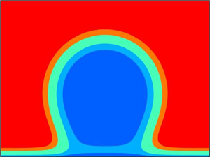
Figure 2. Density profiles of surface nanodrops (a) and nanobubbles (b) at $T=0.6$ ($\varTheta _{{Y}}=105^\circ$), and (left to right) $\Delta \mu =\pm 0.13$ ($R_{{L}}\approx 8$), $\Delta \mu =\pm 0.07$ ($R_{{L}}\approx 15$), $\Delta \mu =\pm 0.04$ ($R_{{L}}\approx 25$), where positive/negative $\Delta \mu$ corresponds to drops/bubbles, respectively. Dotted curves show the arc of a circle, fitted to the liquid–gas interface (density level set at $(\rho _{{l}}+\rho _{{g}})/2$) to compute the apparent radii of the drops, $R^*_{{d}}\approx 8$, $15$, $25$ and bubbles, $R^*_{{b}}\approx 30$, $25$, $32$. The apparent contact angles, $\varTheta ^*_{{d}}=121^\circ$, $114^\circ$, $110^\circ$ and $180^\circ -\varTheta ^*_{{b}}=154^\circ$, $129^\circ$, $118^\circ$, are computed by drawing a tangent (dashed lines) to the circular fit at a distance $1\sigma$ from the wall. The values of $\varTheta ^*_{{d/b}}$ of sufficiently small drops/bubbles are highly sensitive to the technical details of the circle fitting procedure. These values are provided here to illustrate the convergence to $\varTheta _Y$ as the drop/bubble grows.

The shapes of surface drops and bubbles in figure 2 are affected by several factors. The curvature of the liquid–gas interface leads to the $\gamma _{{lg}}/R_{{L}}$ pressure increment inside the adsorbed phase. Therefore, the Laplace radius should provide a good overall estimate of the characteristic dimensions of the drops and bubbles. At the same time, the interface shape, especially near the wall, is the result of a complicated interplay between the liquid–gas and wall–fluid interfaces, such as shown in figure 1(d) for flat films. Indeed, near the substrate, the drop interfaces visibly bend in, whilst the bubble interfaces flatten out, connecting with the thin layer of gas, which covers the outside wall and is induced by the solvation force. This is in agreement with the film adsorption isotherms represented in figure 1(a). Moreover, at small and intermediate sizes, bubbles are significantly flatter than the drops. This happens because the ambient phase interacts very strongly with the substrate in the case of bubbles, ‘squashing’ them.

To test the classical size estimate, given by the Laplace radius, we fit a circle to the liquid–gas interface of surface drops/bubbles and find their ‘apparent’ radii $R^{*}_{{d/b}}$ and contact angles $\varTheta ^{*}_{{d/b}}$. For figure 2 these are reported in the caption, together with the Laplace radii $R_{{L}}$. We introduced a small near-wall cutoff for fitting the circle to avoid the contribution of the ‘flattening’ region near the bubble edges.

Let us note that the values of $R_{{L}}$ are very close for drops and bubbles at the same $|\Delta \mu |$. This means that a description in terms of $R_{{L}}$, which ignores the microscopic details of fluid–substrate interaction, views drop and bubble adsorption in a completely identical way. Interestingly, for small drops this description seems to hold up, as we see a remarkable agreement between $R^{*}_{{d}}$ and $R_{{L}}$ across the drop sizes considered. But the story changes in the case of bubbles where there is hardly any agreement between $R_{{L}}$ and the fitted radius of the two smaller bubbles. Clearly, the fluid–substrate interactions neglected by $R_{{L}}$ are very important for bubbles. Of course, for larger bubbles $R_{{b}}^*$ must start catching up with $R_{{L}}$ (and we can see the beginning of this trend between the bubbles with $R^{*}_{{b}}=25$ and 32), because at saturation the Young contact angle must be recovered. Intuitively, it is clear that the denser liquid above the bubble is attracted to the wall, squashing the bubble. Indeed, this is the intuition behind the binding potential, which we introduce in the next section. This squashing does not happen for drops, because the gas above the drop is too dilute to squash them. We further note that the approach of apparent contact angles to Young values with growing $R^{*}_{{d/b}}$ is also clear and is testament to the accuracy of the DFT computation.

Finally, notice that DFT also elegantly reveals the thermodynamics of drop and bubble nucleation, summarised in figure 1(b). The wall must be dry to act as a nucleation centre for liquid. Accordingly, we find surface drops forming at $(T<T_{{w}},\mu )$ in the red cross-hatched region of figure 1(b). The drop radii are minimal on the liquid film spinodal, and diverge at saturation as ${O}((P(T,\rho _b)-P_{{sat}})^{-1})$, according to the Laplace law. Above $T_{{w}}$, $\varTheta _{{Y}}=0$ and the wall impurity would nucleate a planar wetting film, see, e.g. Yatsyshin et al. (Reference Yatsyshin, Parry and Kalliadasis2016, Reference Yatsyshin, Parry, Rascón and Kalliadasis2017). Surface bubbles can be found in a broader blue-hatched region of figure 1(b), above the gas film spinodal, where their radii are minimal. We can still find surface nanobubbles at $T>T_{{w}}$ and $\mu <\mu _{{sat}}$, but as the wall is completely wet at saturation, such bubbles must detach from the surface at sufficiently small $|\Delta \mu |$.

3. Interface binding potential

In this section we introduce a macroscopic description which corrects the spectacular failure of a description in terms of $R_{{L}}$ for small bubbles, discussed in the previous section and demonstrated in figure 2. We further relate this revised macroscopic description with DFT and show how the two can be used in tandem to describe small systems with diffuse interfaces, high degree of non-uniformity and highly non-local interactions in terms of the intuitive macroscopic concepts of sharp interfaces and biding potentials.

It is noteworthy that with DFT we did not need to stipulate the existence of interfaces, instead the film-, drop- and bubble-like density configurations with diffuse fluid–fluid and fluid–wall interfaces were obtained by solving the non-local DFT equation (2.7). In fact, the formation of these interfaces is the result of local phase separation, occurring because of the correctly chosen bulk thermodynamic point ($T,\mu$), near bulk coexistence and wall wetting transition. An alternative mean-field approach to wetting can be developed by assuming the existence of a sharp liquid–gas interface, with a shape $l(x)$ minimising the excess free energy functional $\varOmega _l[l;T,\mu ]$ of the adsorbate at the given $T$ and $\mu$. Here, $l(x)$ is the distance of the liquid–gas interface from the wall. Such a local approach can be traced back to the early works of Frumkin and Derjaguin (FD; see, e.g. Henderson (Reference Henderson2011) and references therein). Thus, for a system, translationally invariant along the $z$-axis, the interface free energy per unit length can be written in the following general form (see, e.g. Dietrich Reference Dietrich1988; Saam Reference Saam2009)

(3.1)\begin{equation} \varOmega_{l}\left[l;T,\mu\right]=\int_{-\infty}^{+\infty} \left[\gamma_{{lg}}(T) \sqrt{1+\left(\frac{\textrm{d}l}{\textrm{d} x}\right)^2}+W\left(l\left(x\right);T,\Delta\mu\right)\right]{\textrm{d} x}, \end{equation}

where the first term of the integrand is the free energy per unit area of the liquid–gas interface, and the second term is the thermodynamic work of adsorbate formation. Depending on whether the adsorbate is formed of liquid or gas, $W\equiv W_{{liq}}$ or $W\equiv W_{{gas}}$, respectively, with the corresponding volume and surface contributions

(3.2)\begin{equation} W_{{liq/gas}}\left(l\left(x\right);T,\mu\right)=\Delta\mu\Delta\rho(T,\mu)l\left(x\right)+ \gamma_{{wl/g}}(T)+\gamma_{{lg}}(T)+g_{{liq/gas}}\left(l\left(x\right);T\right), \end{equation}

where $g_{{liq/gas}}(l;T)$ is the interface binding potential of liquid/gas film, adsorbed at saturation. It accounts for the interatomic interactions between the liquid–gas interface and the substrate. For LJ forces, $g_{{liq/gas}}(l;T)={O}(l^{-2})$, as $l\to \infty$. The EL equation (3.1) becomes

(3.3)\begin{equation} \frac{\textrm{d}^2 l}{{\textrm{d} x}^2}=\frac{1}{\gamma_{{lg}}}\left(1+\left(\frac{\textrm{d} l}{\textrm{d} x}\right)^2\right)^{{3}/{2}}\dot{W}\left(l;T,\mu\right), \end{equation}

where $\dot {W}(l;T,\mu )$ denotes the derivative of $W(l;T,\mu )$ with respect to $l$. Equation (3.3) has been referred to as the augmented Young–Laplace equation by Wu & Wong (Reference Wu and Wong2004), i.e. the standard Young–Laplace equation modified to include the disjoining pressure. Here, we shall refer to (3.3) as the FD equation because we establish the connection between the microscopic free energy in (2.1) and the macroscopic DF free energy in (3.1), which in turn leads to (3.3). Without consideration of the free energies, this link cannot be established as disjoining pressure is typically associated with the formation of thin films.

If ${W}(l;T,\mu )$ is known, the FD equation (3.3) can be integrated from the absolute minimum of ${W}(l;T,\mu )$, until $\textrm {d}l/{\textrm {d} x}$ becomes constant. Notice that, when $\dot {W}\equiv 1$, (3.3) defines a circle of curvature $\gamma _{{lg}}^{-1}$, and when $\dot {W}\equiv 0$, it defines a straight line. Therefore, at $\mu _{{sat}}$ the solution must tend to a flat liquid–gas interface, and below/above $\mu _{{sat}}$, it must trace a circular-like shape of a drop/bubble. From (3.3), it follows that the curvature of the sharp interface $l(x)$ is given by $\dot {W}/\gamma _{{lg}}$, where according to (3.2) and the definition of $R_{{L}}$, $\dot {W}\approx \gamma _{{lg}}/R_{{L}}+\dot {g}$. Thus, $\dot {g}/\gamma _{{lg}}$ has a nice interpretation as the curvature correction to the circular shape of the drop/bubble of Laplace radius, induced by the presence of the substrate.

We can compute the work of film formation $W_{{liq}}(l;T,\mu )$ and $W_{{gas}}(l;T,\mu )$ from DFT, using the same density profiles in $\{\rho (x)\}_T^{{gas}}$ and $\{\rho (x)\}_T^{{liq}}$ that give rise to the liquid- and gas-adsorption isotherms, such as shown in figure 1(a). This requires us to make an ansatz about the density and free energy density profiles of a liquid (or gas) film, of a given height $l$, adsorbed on the wall at the given $T$ and $\mu$. All we know is that such film must be thermodynamically unstable, unless all three, $l$, $\mu$ and $T$, belong to a (meta)stable branch of an adsorption isotherm. If we ignore the fact that each profile in the isotherm sets is associated with a particular chemical potential and treat $\mu$ as fixed, the sets $\{\rho (x)\}_T^{{gas}}$ and $\{\rho (x)\}_T^{{liq}}$ turn out to contain the density profiles of (now unstable) adsorbed films of different widths. Moreover, these density profiles retain the key features of the LJ model of adsorption: a nearly flat plateau at the density of the adsorbed phase, followed by a diffuse liquid–gas interface, consistent with $T$, and an inverse cubic rate of decay to bulk density. Also, the near-wall fluid structure and the interaction of the fluid–wall and liquid–gas interfaces at small $l$ are keeping in touch with the underlying DFT functional. Note that since $\mu$ is fixed, the large-$x$ limit of the density profiles so chosen do not coincide with the bulk density at $\mu$. This is not a problem, because $W(l;T,\mu )$ is the free energy of the adsorbed film, so the bulk contribution has to be removed anyway. At the same time, the rate of decay of the density profile to its asymptote is important.

Thus, given $T$, $\mu$ and a profile $\rho _0(x)$ from $\{\rho (x)\}_T^{{gas}}$ or $\{\rho (x)\}_T^{{liq}}$, which solves the EL equation (2.7) at the required $T$ and some $\mu _0$, we need to compute the height $l$ of the adsorbed film, and its free energy $W(l;T,\mu )$. Associated with $\rho _0(x)$ are its limit $\rho ^0_{{b}}=\lim _{x\to \infty }{\rho _0(x)}$, adsorption $\varGamma _0=\int _0^\infty (\rho _0(x)-\rho _{{b}}^0)\,{\textrm {d} x}$, and the grand free energy density $\omega (x;\rho _0(x),T,\mu _0)$, defined in (2.11). It is reasonable to set $l=\varGamma _0/\Delta \rho (T,\mu )$, because then $l$ is related to the physical bulk density (given by $T$ and $\mu$) and correctly recovers $l_0(T,\mu _{{sat}})$ and $l_0(T,\mu _0)$, see (2.10). Additionally, this ensures that $l$ cannot be ‘computed’ in the region outside the bulk spinodals, where metastable phases (and thus $\Delta \rho$) do not exit. The free energy of the adsorbed film can be obtained from $\varOmega [\rho _0(x);T,\mu ]$ in (2.1) by removing the contribution of gas on the outside of the liquid–gas interface. Because the liquid–gas interface is diffuse, simply limiting the integration interval to $[0,l]$ will be incorrect. The solution is to work instead with the grand free energy density, $\omega (x;\rho _0(x),T,\mu _0)$, defined in (2.11). Notice that for large $x$, $\omega (x;\rho _0(x),T,\mu)= -P(\rho _{{b}}^0, T)+ (\mu _0-\mu )\rho _{{b}}^0+{O}(1/x^3)$ as $x\to \infty$. Removing this bulk contribution, we get $W(l;T,\mu )$ by integration

(3.4)\begin{equation} \left.\begin{gathered} W(l;T,\mu)=\int_0^{\infty}\left[\omega(x;\rho_0,T,\mu)-\left({-}P(\rho_{{b}}^0, T)+(\mu_0-\mu)\rho_{{b}}^0\right) \right]{\textrm{d} x},\\ l = \int\left(\rho_0(x)-\rho_{{b}}^0\right)/\Delta\rho(T,\mu). \end{gathered}\right\} \end{equation}

Repeating this computation for every profile in $\{\rho (x)\}_T^{{gas}}$ and $\{\rho (x)\}_T^{{liq}}$, we tabulate the respective work of gas and liquid film formation, $W^{{gas}}(l;T,\mu )$ and $W^{{liq}}(l;T,\mu )$.

In figure 3 we represent the work of film formation at $T=0.85$, and $\Delta \mu =0$ and $\Delta \mu =-0.035$, together with solutions of the FD equation (3.3). The curves $W_{{liq}}(l;T,\mu )$ (green-grey-red) and $W_{{gas}}(l;T,\mu )$ (blue-grey), and the FD interfaces $l_{{liq}}(x)$ and $l_{{gas}}(x)$, obtained using them, are coloured as the isotherms $l_{{liq}}(\mu )$ and $l_{{gas}}(\mu )$ in figure 1(a) at respective $l$. For illustration purposes, we have shifted the curves $l_{{gas}}(x)$ along the $x$-axis to facilitate visual comparison with $l_{{liq}}(x)$. Notice that the unstable parts of $W(l;T,\mu )$ curves (grey) are concave, and separated from the convex stable parts (coloured) by the inflection points (filled circles), which correspond to the spinodals of $l(\mu )$. Local extrema of $W(l;T,\mu )$ (open circles) correspond to the intersections of $l(\mu )$ with lines $\Delta \mu =0$ and $\Delta \mu =-0.035$. In fact, the qualitative behaviour of $W(l;T,\mu )$ and $l(x)$ is apparent from figure 1(a): intersections of isotherms with vertical lines $\mu =\textrm {const.}$ must correspond to alternating minima and maxima of $W(l;T,\mu )$.

Figure 3. The curve colours and open/filled circles here correspond to those in figure 1(a) at the same $l$. (a,c) Work of formation of liquid film, $W_{{liq}}(l;T,\mu )$ (green-grey-red curves), and gas film, $W_{{gas}}(l;T,\mu )$ (blue-grey curves) at $T=0.88$ ($\varTheta _{{Y}}=50.6^\circ$). (b,d) Liquid–gas interfaces, obtained from (3.3) with $W = W_{{liq}}$ and $W = W_{{gas}}$, and coloured accordingly. In (a,b) $\Delta \mu =0$, and in (c,d) $\Delta \mu =-0.035$. The spinodals of $l(\mu )$ in figure 1(a) correspond to the inflection points of $W$ (filled circles), and the intersections of $l(\mu )$ with lines $\Delta \mu =0$ and $\Delta \mu =-0.035$ correspond to the extrema of $W$ (open circles). The asymptotes of $W$ are indicated by dashed lines. In (a), the limits and minima of $W(l;T,\mu _{{sat}})$ are indicated by text; the inset shows the decay of $W(l;T,\mu _{{sat}})$ on a log–log plot, where the black dashed line is a guide to eye at the expected asymptotic decay $W\propto 1/l^2$.

At saturation (figure 3a) the volume contribution to $W(l;T,\mu )$ vanishes, and $W_{{liq}}(l;T,\mu _{{sat}})$ and $W_{{gas}}(l;T,\mu _{{sat}})$ tend to the respective sums of the liquid–gas and fluid–wall surface tensions, as $l\to \infty$. The inverse quadratic rate of decay of $W_{{liq}}(l;T,\mu _{{sat}})$ can be verified numerically, as shown in the inset of figure 3(a). Subtracting these asymptotes from $W_{{liq}}(l;T,\mu _{{sat}})$ and $W_{{gas}}(l;T,\mu _{{sat}})$, would yield the interface binding potential, which turns out to have two branches, associated with liquid and gas adsorption, respectively. The local minima of $W_{{liq}}(l;T,\mu _{{sat}})$ at $W_{{liq}}=\gamma _{{wg}}$ and that of $W_{{gas}}(l;T,\mu _{{sat}})$ at $W_{{gas}}=\gamma _{{wl}}$ reflect the fact that when saturation is approached from the gas/liquid phase, the wall is covered by a stable layer of liquid/gas, respectively (see green/blue branch in figure 1a). Since the attractive wall favours liquid, this minimum of $W_{{gas}}(l;T,\mu _{{sat}})$ must always be global. On the other hand, the first-order wetting transition brings about a competing minimum of $W_{{liq}}(l;T,\mu _{{sat}})$ at $l\to \infty$, which becomes global at $T\geqslant T_{{w}}$.

The stability of liquid and gas films, expressed by the work of film formation and, equivalently, by the adsorption isotherms, directly translates into the near-substrate shapes of the liquid–gas interfaces $l(x)$, depicted in figure 3(b). At saturation, $l_{{liq}}(x)$ must have an inflection point at the same $l$, where $W_{{liq}}(l;T,\mu _{{sat}})$ has a local maximum. The existence of such local maximum directly follows from the fact that the binding potential must have two minima to allow for first-order wetting transition. On the other hand, $l_{{gas}}(x)$ cannot have an inflection point at saturation, because $W_{{liq}}(l;T,\mu _{{sat}})$ must monotonically approach $\gamma _{{wg}}+\gamma _{{lg}}$ after reaching its local minimum (there is no coexistence between adsorbed gas films). As mentioned above, the starting point on each $l(x)$ is at the minimum of the respective $W$ (marked by open circle), and the numerical solution is stopped when the change of $\textrm {d}l/{\textrm {d} x}$ is below machine tolerance. Since at saturation, $\dot {W}(l)\to 0$ with $l$ as ${O}(1/l^3)$, $l(x)$ must tend to a straight line with an inclination angle $\varTheta _{{Y}}$ to the $x$-axis. Numerically we find that $\varTheta _{{Y}}$, predicted by DFT is reached by $l(x)$ with a remarkable accuracy.

Off of saturation $W(l;T,\mu )$ can be computed by applying (3.4), or from $W(l;T,\mu _{{sat}})$, by subtracting the volume term $\Delta \mu \Delta \rho l$ and rescaling $l$ appropriately. In figure 3(c) we applied (3.4) and verified numerically that $W(l;T,\mu )$ has the linear asymptotes $\Delta \mu \Delta \rho l$ (dashed lines). Notice that here the volume term creates a local maximum for $W_{{gas}}(l;T,\mu )$ and eliminates it for $W_{{liq}}(l;T,\mu )$. As a result, the interface line $l_{{gas}}(x)$ has an inflection point but $l_{{liq}}(x)$ does not (figure 3d). The interface lines must have ‘near-circular’ shapes when the volume term is non-zero, because if $\dot {W}(l;T,\mu )$ is a constant, (3.3) defines a circle.

The interfaces $l_{{liq}}(x)$ and $l_{{gas}}(x)$ differ substantially near the wall, reflecting the fact that the wetting transition and thin–thick film coexistence affects $W_{{liq}}(l;T,\mu )$, but not $W_{{liq}}(l;T,\mu )$. Notice also that the effect of the solvation force, locally repelling the liquid from the wall, leads to a higher near-wall part of $l_{{gas}}(x)$, than $l_{{liq}}(x)$ in figures 3(b) and 3(c). The DF model captures this effect via the properly computed work of film formation, where the local minimum of $W_{{gas}}(l;T,\mu )$ is reached at a slightly higher $l$, than that of $W_{{liq}}(l;T,\mu )$. It is noteworthy that the part of $l_{{liq}}(x)$ between the near-wall region (green) and the outer liquid–gas region (red) is determined by the density profiles $\rho (x)$ from the saddle manifold of $\varOmega [\rho (x)]$. Thus, the mean-field DFT functional allows us to connect these metastable states in a non-ambiguous way. In the case of $l_{{gas}}(x)$, the density profiles from the saddle manifold of $\varOmega [\rho (x)]$ determine most of the liquid–gas interface.

In figure 4 we represent a direct comparison between the DFT density profiles and DF interface lines $l_{{liq}}(x)$ (dashed) and $l_{{gas}}(x)$ (dotted), obtained at the same $T$ and $\mu$. To superimpose the DF interfaces over $\rho (x,y)$, we aligned the tops of $l_{{liq}}(x)$ and $l_{{gas}}(x)$ (where $\textrm {d}l/{\textrm {d} x}$ vanish) with $x=0$. We also reflected some $l(x)$ with respect to the $y$-axis, so that $l_{{liq}}(x)$ and $l_{{gas}}(x)$ appear in $x\leqslant 0$ and $x\geqslant 0$ half-planes of each plot, respectively. In figures 4(a)–4(c) we show nanodrops and nanobubbles of the same height $30\sigma$ at two different temperatures below $T_{{w}}$. Overall, the local DF model captures well the heights of the drops and bubbles, and the changes of the interface curvature at small scales. As can be seen, $\rho (x,y)$ possesses level sets which closely resemble both $\rho _{{liq}}$ and $\rho _{{gas}}$. Interestingly, no part of $l_{{liq}}(x)$ can be found between the wall and liquid, just as no part of $l_{{gas}}(x)$ is found between the wall and gas. This is a limitation of the local functional $\varOmega _l[l]$, which does not allow $l(x)$ to bifurcate. Another limitation of the DF model, not apparent from figure 4, was already mentioned above: our treatment of repulsions in (2.2) cannot capture the near-wall layering of the fluid density associated with the excluded volume intermolecular correlations. This is because our DFT functional was chosen specifically to capture the liquid–gas interface, without the unnecessary complications of the finer near-wall details, which are irrelevant for the present study. Investigating the low-temperature regime, where the near-wall layering is important certainly presents interesting questions for further study, beyond the scope of the present work.

Figure 4. Comparison between DFT (coloured contour plots) and DF model (black curves). In each plot, dashed and dotted black curves to the left and right of the white vertical line at $x=0$ correspond to $l_{{liq}}(x)$ and $l_{{gas}}(x)$, respectively. In (a–d) $T<T_{{w}}$; the drops and bubbles have the same average height $30\sigma$. In (e,f) $T>T_{{w}}$, and we see a nucleation cluster of the flat prewetting film, and a detaching bubble. Thermodynamic points: (a,b) $T=0.65$ ($\varTheta _{{Y}}=101^\circ$), $\Delta \mu =-2.4\times 10^{-2}$ and $3.8\times 10^{-2}$; (c,d) $T=0.85$ ($\varTheta _{{Y}}=65^\circ$), $\Delta \mu =-1.8\times 10^{-2}$ and $0.9\times 10^{-2}$; (d,f) $T=0.93$ ($\varTheta _{{Y}}=0^\circ$, $\Delta \mu _{{pw}}=-1.4\times 10^{-3}$), $\Delta \mu =-8.5\times 10^{-4}$ and $-1.0\times 10^{-2}$.

It is very important to understand that a local model, such as DF cannot in principle be expected to replace a statistical-mechanical method, such as DFT. An excellent example illustrating the tight limits of applicability of local models is provided by the continuous prewetting transition (Yatsyshin et al. Reference Yatsyshin, Parry and Kalliadasis2016). Since we have a microscopic drop on a substrate, it must nucleate a thin liquid film at $\mu _{{pw}}$ and $T>T_{{w}}$ (see figure 1a,b). While DFT captures the onset of such prewetting without any problem, the DF model breaks down, because it does not include the interactions between different points on the interface. In figure 4(e) we depict a nucleation cluster of the flat prewetting film above $T_{{w}}$. The round edges of the adsorbed liquid structure are deceptive. Fitting a circle to the liquid–gas interface as in figure 2, we get $R^*=49\sigma$. At the same time, the Laplace radius is $R_{{L}}=225\sigma$, testifying to the fact that what we see is indeed a forming flat film. The work $W_{{gas}}(l;T,\mu )$ does not include the bi-stability of wetting liquid films, and as a result $l_{{gas}}(x)$ fails to capture the lateral extent of the film. This failure of $l_{{gas}}(x)$ near the prewetting transition is systematic in our study and manifests the highest disagreement between the DF and DFT models.

Rather surprisingly, we find a remarkable agreement between the local DF and non-local DFT in the case of a nearly detached nanobubble, shown in figure 4(e) (since $\varTheta _{{Y}}=0$, the surface bubbles will detach as $\Delta \mu \to 0$). The DF interface lines here are $S$-shaped (although still single valued if treated as functions of $y$), as are the level sets of $\rho (x,y)$. This is curious, because the local free energy $\varOmega _l$ does not account for the self-interaction in the liquid–gas interface, and the agreement between DF model and DFT should have broken down. It follows that such $S$-shaped profiles are the consequence of the change of sign of $\dot {W}$ in (3.3), and do not necessarily require including curvature and self-interaction effects into the interfacial free energy $\varOmega _l$.