2. Methodology

In this paper, we use the well-validated VoF solver (Zeng et al. Reference Zeng, Gonzalez-Avila, Dijkink, Koukouvinis, Gavaises and Ohl2018a,Reference Zeng, Gonzalez-Avila, Ten Voorde and Ohlb, Reference Zeng, Gonzalez-Avila and Ohl2020; Gonzalez-Avila et al. Reference Gonzalez-Avila, van Blokland, Zeng and Ohl2020) to conduct a study of the wall shear stress generated from expanding and collapsing cavitation bubbles as a function of viscosity and initial distance to a solid boundary. The problem consists of two phases (gas and liquid), where both are compressible and immiscible Newtonian fluids. As heat and mass transfer between two phases are negligible (Koukouvinis et al. Reference Koukouvinis, Strotos, Zeng, Gonzalez-Avila, Theodorakakos, Gavaises and Ohl2018; Zeng et al. Reference Zeng, Gonzalez-Avila and Ohl2020), the governing equations for the flow are the equations of continuity and momentum:

(2.1)$$\begin{gather} \frac{\partial \rho}{\partial t}+\boldsymbol{\nabla}\boldsymbol{\cdot}(\rho \boldsymbol{u})=0, \end{gather}$$

(2.2)$$\begin{gather}\frac{\partial \rho \boldsymbol{u}}{\partial t}+\boldsymbol{\nabla}\boldsymbol{\cdot}(\rho \boldsymbol{uu})={-}\boldsymbol{\nabla} p +\boldsymbol{\nabla}\boldsymbol{\cdot}\boldsymbol{s} + \boldsymbol{f_\delta}, \end{gather}$$

where $\rho, \boldsymbol {u}, t$ and $p$ are the density, velocity, time and pressure, respectively. The role of viscosity is included as the viscous stress tensor $\boldsymbol {s}=\mu [\boldsymbol {\nabla } \boldsymbol {u}+\boldsymbol {\nabla } \boldsymbol {u}^T-\frac {2}{3}(\boldsymbol {\nabla }\boldsymbol {\cdot } \boldsymbol {u})\boldsymbol {I}]$, with the dynamic viscosity $\mu$ and an identity tensor $\boldsymbol {I}$. Here, $\boldsymbol {f_\delta }$ is the surface tension term modelled with the so-called continuous surface force (CSF) method (Brackbill, Kothe & Zemach Reference Brackbill, Kothe and Zemach1992).

The cavitation bubble content is numerically treated as a non-condensable gas, which follows a polytropic equation of state (EOS):

(2.3)\begin{equation} \frac{p}{\rho^\kappa} = \frac{p_n}{\rho_n^\kappa},\end{equation}

where $p_n=101325$ Pa and $\rho _n=1.2$ kg m$^{-3}$ are the reference pressure and density of the gas, $\kappa =1.4$ is the specific heat ratio or adiabatic exponent of the gas phase and the surrounding liquid is modelled as a Tait-compressible liquid:

(2.4)\begin{equation} \rho=\rho_0\left(\frac{p+B}{p_0+B}\right)^{1/\varGamma},\end{equation}

where $p_0=101325$ Pa and $\rho _0=1000$ kg m$^{-3}$ are the reference density and reference pressure, respectively. Here, $\varGamma =7.15$ is the Tait exponent and $B=3046$ bar is the Tait pressure. To capture the bubble interface, a transport equation for the volume fraction of the liquid phase $\alpha$ is solved (Miller et al. Reference Miller, Jasak, Boger, Paterson and Nedungadi2013; Koch et al. Reference Koch, Lechner, Reuter, Köhler, Mettin and Lauterborn2016; Zeng et al. Reference Zeng, Gonzalez-Avila, Ten Voorde and Ohl2018b):

(2.5)\begin{equation} \frac{\partial \alpha}{\partial t}+\boldsymbol{\nabla}\boldsymbol{\cdot}(\alpha \boldsymbol{u})+\boldsymbol{\nabla}\boldsymbol{\cdot}(\alpha(1-\alpha)\boldsymbol{U_r})= \alpha(1-\alpha)\left(\frac{\psi_g}{\rho_g} -\frac{\psi_l}{\rho_l} \right) \frac{\textrm{D}p}{\textrm{D}t}+\alpha\boldsymbol{\nabla}\boldsymbol{\cdot} \boldsymbol{u}, \end{equation}

where $\psi =\textrm {D}\rho /\textrm {D}p$ is the compressibility computed based on the EOS. The subscripts $l$ and $g$ represent the liquid and the gas phases, respectively, and $\boldsymbol {U_r}$ is the relative velocity between two phases and acts as an artificial compressible term ensuring a sharp interface (Rusche Reference Rusche2003).

Simulations were performed using OpenFOAM (Weller et al. Reference Weller, Tabor, Jasak and Fureby1998), where the compressible Navier–Stokes (NS) equations are discretized and solved with the VoF method to obtain the velocity and pressure field and the time-dependent bubble interface. The EOS was used to compute the compressibility and density of each phase based on the pressure. When solving the equations, the time step is adaptively updated by specifying the Courant number as 0.1 to ensure the stability of the solution. Details of the numerical method are documented in Zeng et al. (Reference Zeng, Gonzalez-Avila, Dijkink, Koukouvinis, Gavaises and Ohl2018a,Reference Zeng, Gonzalez-Avila, Ten Voorde and Ohlb, Reference Zeng, Gonzalez-Avila and Ohl2020).

The bubbles studied here have a maximum equivalent radius $R_{max}\approx 400\ \mu$m similar to those in Reuter & Kaiser (Reference Reuter and Kaiser2019). To simplify the simulation and limit the effects from distant boundaries, we choose an axisymmetric domain of $10\ \textrm {mm}\times 10\ \textrm {mm}$. The mesh is refined successively so that it has a finer spacing of $\Delta x=1.5\ \mu$m closer to the bubble but coarsens quickly further away. This non-uniform mesh allows us to conduct high-resolution simulations with moderate computational resources. The initial bubble is nucleated as a high-pressure gas sphere with its centre located at a distance of $d$ from the wall, therefore at a non-dimensional stand-off distance $\gamma =d/R_{max}$. The rigid wall below the bubble is modelled as a no-slip boundary. The near-boundary mesh is gradually refined even further down to a spacing of $\Delta x=50$ nm to make sure that the boundary layer flow for the expected high values of the strain rates is resolved adequately. Outer boundaries are considered far fields. Vanishing gradient of velocities are applied at outer boundaries to allow in and out flux. For pressure field, the vertical and radial outer boundaries are set as the ambient pressure $P_\infty =101325$ Pa and a non-reflecting boundary, respectively. The gas bubble is initialized with a radius $R(t=0)=25\ \mu$m and a high pressure $P_0$. The high pressure $P_0$ is adjusted to meet the experimental period of growth and collapse of each bubble in § 3 but is kept constant as $P_0=2700$ bar for the remaining sections.

3. Fluid flow near the wall

The model is first tested against bubbles collapsing for $\gamma \le 1.1$ near a rigid boundary. Reuter & Kaiser (Reference Reuter and Kaiser2019) not only measured the bubble shape but also the thickness of the liquid film separating the bubble from the rigid boundary. Two of their high-speed recordings are shown in figure 1 for $\gamma =1.05$ and $\gamma =0.56$. The red contours are the bubble interface superimposed on the experimental recording that are taken from the simulations at the same time instance. In figure 1($a$) for $\gamma =1.05$, the bubble expands to a nearly spherical shape then shrinks into an elongated bubble with the larger axis oriented normal to the boundary. In the second comparison, figure 1($b$) checks the simulation against a bubble nucleated closer to the solid boundary with $\gamma =0.56$. During the expansion, the bubble flattens considerably its lower surface and takes the shape of nearly a hemispherical bubble that changes into a cone-shaped outline before collapsing as a toroidal bubble.

Figure 1. Comparison of the computed bubble dynamics and experimental results from Reuter & Kaiser (Reference Reuter and Kaiser2019). Red contours represent the computed bubble interface. Dashed lines indicate the positions of the solid boundaries. $(a)$ Experiment –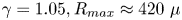$\gamma =1.05, R_{max} \approx 420\ \mu$m; simulation –$\gamma =1.05, R_{max}= 410\ \mu$m, $P_0=2900$ bar. $(b)$ Experiment –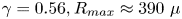$\gamma =0.56, R_{max} \approx 390\ \mu$m; simulation –$\gamma =0.57, R_{max}= 380\ \mu$m, $P_0=2300$ bar.

While the agreement with the overall shape of the bubble is a good indicator for the quality of the simulation, the liquid flow very close to the boundary is crucial for obtaining good estimates of the wall shear stress. We therefore compare the thickness of the thin liquid film that separates the bubble from the rigid boundary. Figure 2$(a)$ plots the minimum time-dependent thickness, $h(t)$, of the thin film for four pairs of very similar stand-off distances. The lines decorated with dots are the experimental data from Reuter & Kaiser (Reference Reuter and Kaiser2019) while solid lines are from simulations. During the early expansion, $h(t)$ drops rapidly for all cases. The decrease slows down in the late expansion. In the later dynamics, $h(t)$ approaches a constant value during collapse for $\gamma \leq 1$, but it increases at the late collapse for $\gamma =1.2$. These two distinct dynamics result in two different functions of the film thickness at jet impact (see below and figure 2$b$). Please note that in the measurement of Reuter & Kaiser (Reference Reuter and Kaiser2019), a flat mirror-like bubble interface is assumed while this is only approximately true. Therefore the measurement overestimates $h(t)$ when the lower bubble interface is curved, which for small stand-off distances is the case only during the early stage of the bubble expansion. For larger stand-off distances, the film is considerably curved (see figure 1$a$).

Figure 2. Liquid film dynamics. $(a)$ The evolution of the gap thickness for different $\gamma$ values, lines represent the simulation data while lines with dots are the measurement from Reuter & Kaiser (Reference Reuter and Kaiser2019); the experimental and simulation data end at the time of jet impact. In the experiment, $R_{max}= 411, 419$ and 406 $\mu$m, for $\gamma = 0.56$, 0.76 and 0.99, respectively; in the simulation, $R_{max}= 409$, 417, 405 and 397$\mu$m for $\gamma = 0.56$, 0.76, 0.99 and 1.2, respectively. $(b)$ The gap thickness at jet impact onto the bubble's lower interface, solid line is the fit provided by Reuter & Kaiser (Reference Reuter and Kaiser2019) ($\gamma =0.47 - 1.07$) and the slope of the green dashed line is 1.

Next we have a look at the film thickness at the moment the jet contacts the bubble's lower interface, $h_{jet}$. This is the time just prior to the jet impact when high normal and shortly afterward tangential stresses are experienced by the boundary. Figure 2$(b)$ compares the measured film thickness $h_{jet}$ normalized by the maximum bubble radius $R_{max}$ with the simulations (dots). The solid line up to $\gamma =1.1$ are the empirical correlation found by Reuter & Kaiser (Reference Reuter and Kaiser2019), which is $h=29.2\gamma ^{4.86}+4.74$ ($\mu$m) for bubbles with $0.47<\gamma <1.07$. This fit is based on 91 experiments with bubble sizes in the interval $385\ \mu\text {m}< R_{max}<435\ \mu\text {m}$ with a mean size of $410\ \mu$m. The simulations are spot on with this empirical fit. Continuing the simulations to larger $\gamma$ values, we find an approximately linear increase of the height as indicated with the dashed line in figure 2$(b)$.

4. Viscous bubble dynamics

Previously, a detailed study of the bubble dynamics and the resulting distribution of the wall shear stress was done for a few selected cases in water at a distance of $\gamma \approx 1$ (Zeng et al. Reference Zeng, Gonzalez-Avila, Dijkink, Koukouvinis, Gavaises and Ohl2018a). The choice of $\gamma$ value was motivated for a comparison with an experiment. In the present work, we expand the study to reveal the effect of liquid viscosity $\mu$ (from $10^{-3}\ \mathrm {Pa}\cdot \textrm {s}$ to $0.1\ \mathrm {Pa}\cdot \textrm {s}$) and stand-off distance $\gamma$ (from $\gamma =0.5$ to 1.6). The choice of the parameter space is to cover the important transitions (see below sections) while practical for bubble nucleation. For all simulations present below, the initial pressure within the bubble is fixed to 2700 bar, i.e. the initial energy is the same for all simulations. Owing to viscous dissipation, the resulting maximum equivalent radius $R_{max}$ increases slightly from $370\ \mu$m to $400\ \mu$m with decreasing viscosity.

Now we look at how the liquid viscosity influences the bubble dynamics. Here we define the Reynolds number 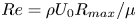$Re=\rho U_0 R_{max}/\mu$, where $U_0=\sqrt {P_\infty /\rho }$ is a referenced velocity from the ambient pressure $P_\infty$ and $R_{max}$ the maximum bubble radius of each simulation. The dimensionless numbers chosen here are related to the shrinkage instead of the growth of the bubble, similar to Jayaprakash, Hsiao & Chahine (Reference Jayaprakash, Hsiao and Chahine2012).

In figure 3, we show the comparison of the bubble's equivalent radius for three different viscosities for two selected stand-off distances $\gamma =0.7$ and $\gamma =1.1$. It is seen at both $\gamma$ values that the bubble dynamics is slowed down and $R_{max}$ reduces with increasing viscosity, which is the result of the increasing viscous drag and dissipation (Brennen Reference Brennen2014). Although the evolution of the bubble radius changes only mildly with an increase of liquid viscosity, i.e. from 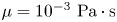$\mu =10^{-3}\ \textrm {Pa} \cdot \textrm {s}$ to $\mu =0.02\ \textrm {Pa} \cdot \textrm {s}$, we find a significant difference in the bubble shape, as shown in figures 4 and 5.

Figure 3. Comparison of bubble's equivalent radius for different viscosities: $(a)\ \gamma =0.7; (b)\ \gamma =1.1$. The bubble dynamics for $\mu =10^{-3}\ \textrm {Pa} \cdot \textrm {s}$ is drawn in both plots for comparison. The $R_{max}$ is $394\ \mu$m, $388\ \mu$m, 385$\ \mu$m in panel (a), and $396\ \mu$m, $390\ \mu$m, $386\ \mu$m in panel (b) for viscosity 0.001, 0.02, $0.04\ \textrm {Pa} \cdot \textrm {s}$, respectively.

Figure 4. Comparison of the computed bubble shapes for $\gamma =0.7$ between $\mu =10^{-3}\ \textrm {Pa} \cdot \textrm {s}$ (black shapes) and $\mu =0.02\ \textrm {Pa} \cdot \textrm {s}$ (red lines). Times are in $\mu$s. The lower borderline of each frame represents the solid boundary. The maximum bubble radius $R_{max}$ reduces from $394\ \mu$m to $388\ \mu$m with increasing viscosity.

Figure 5. Comparison of the computed bubble shapes for $\gamma =1.1$ between $\mu =10^{-3}\ \textrm {Pa} \cdot \textrm {s}$ (black shapes) and $\mu =0.02\ \textrm {Pa}\cdot \textrm {s}$ (red lines). Times are in $\mu$s. The lower borderline of each frame represents the solid boundary. The maximum bubble radius $R_{max}$ reduces from $396\ \mu$m to $390\ \mu$m with increasing viscosity.

Figure 4 plots the bubble shapes from expansion to collapse for the same stand-off distance $\gamma =0.7$ but two different viscosities ($\mu =10^{-3}\ \textrm {Pa} \cdot \textrm {s}$, black shape; 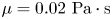$\mu =0.02\ \textrm {Pa} \cdot \textrm {s}$, red contour). Bubbles in both liquids acquire an hemispherical shape and collapse into a conical and toroidal shape sequentially, but a clear difference is visible during this dynamics. First of all, the motion of the top interface moving towards the wall is slowed in the more viscous liquid owing to higher viscous drag, which leads to a lower jet impact velocity. The dynamics in the near-wall region is greatly affected by the liquid viscosity too, which is attributed to the thicker boundary layer formed in the more viscous liquid. It is seen that the liquid film thickness $h_{jet}$ increases from $8\ \mu$m to $20\ \mu$m when the liquid viscosity changes from $\mu =10^{-3}\ \textrm {Pa} \cdot \textrm {s}$ to $\mu =0.02\ \textrm {Pa}\cdot \textrm {s}$. Additionally, the bubble edge becomes smoother and is lifted further from the wall vertically but closer to the axis horizontally.

A second comparison of the bubble shapes is plotted in figure 5 for a higher stand-off distance $\gamma =1.1$. Here, we also observe a slower bubble motion and an increase of the liquid film thickness $h_{jet}$ from $53\ \mu$m to $75\ \mu$m when the liquid viscosity changes from $\mu =10^{-3}\ \textrm {Pa} \cdot \textrm {s}$ to a 20 times more viscous liquid $\mu =0.02\ \textrm {Pa} \cdot \textrm {s}$. Interestingly, owing to the stronger viscous drag, the bubble becomes spherical instead of elongated in the more viscous liquid during the early collapse ($42< t<80\ \mu$s). Yet at a later time but before the jet formation ($t=80\ \mu$s), the bubble interface at the axis collapses slower than the nearby interface and the top interface acquires a particular curvature. This arises from a combined effect of viscous drag and the flow induced by the shrinking bubble. Such a curvature may result into a higher jet velocity although occurring in a more viscous liquid, see figure 6$(b)$.

Figure 6. Influence of $1/Re$ number on four important features of the bubble dynamics for two selected stand-off distances $\gamma =0.7,1.1$. $(a)$ Film thickness, $(b)$ jet velocity, $(c)$ width of the jet and $(d)$ volume of the jet, where $V_{max}$ is the bubble volume at maximum expansion. The inset in panel $(c)$ sketches the definition of jet width and volume, similar to Jayaprakash et al. (Reference Jayaprakash, Hsiao and Chahine2012).

Figure 6 depicts the influence of viscosity on four important features of the bubble dynamics for the two selected stand-off distances $\gamma =0.7$ and $\gamma =1.1$. In figure 6$(a)$, the film thickness is found to increase with viscosity for both $\gamma$ values and becomes constant in the high $1/Re$ regime for $\gamma =1.1$. Figure 6$(b)$ reveals that the jet velocity, in general, decreases with viscosity and increases with $\gamma$. Interestingly, we found one special case ($\gamma =1.1$ the second marker) where the jet velocity could increase in a more viscous liquid, whose mechanism is related to the particular curved top interface motioned above. The structures of the jet are plotted in figure 6(c,d) with the inset depicting the geometry. The normalized jet width $R_{jet}/R_{max}$ for both $\gamma$ values fluctuates around 0.3. Yet in a low viscous liquid, a smaller $\gamma$ has a wider jet width, and this trend and the magnitude agree with the findings reported by Jayaprakash et al. (Reference Jayaprakash, Hsiao and Chahine2012). The normalized jet volume shown in figure 6$(d)$ decreases with $1/Re$. The reason is that in the more viscous liquid, the jet formation slows down so the bubble has collapsed into a smaller size when the impact occurs. The local minimum at low $1/Re$ for $\gamma =1.1$ (the second and third markers) is the result of the particular shape of the bubble shown in figure 5.

In figure 7, we summarize the values of $h_{jet}$ in $(a)$ and $U_{jet}$ in $(b)$, which are the main factors on the formation of the wall shear stress and used for further analysis in § 6 below. At low $\gamma, h_{jet}$ increases with $1/Re$ while is almost constant at high $\gamma$. Overall, the jet velocity $U_{jet}$ decreases with viscosity and increases with $\gamma$, so $h_{jet}$ and $U_{jet}$ are both a complex function of these two parameters. The results for a low-viscosity liquid are consistent with experiments (Philipp & Lauterborn Reference Philipp and Lauterborn1998) and simulations (Lechner et al. Reference Lechner, Lauterborn, Koch and Mettin2020).

Figure 7. The distribution of normalized gap thickness $h_{jet}/R_{max}$ and jet velocity $U_{jet}/U_{0}$ on ($1/Re, \gamma$).

The result here also alerted us to the use of an inviscid model for $\gamma <1$ in the low $1/Re$ regime. Although the viscous damping plays a minor role in the low $1/Re$ regime, the formation of a thin film separating the bubble and the wall strongly relies on the appearance of liquid viscosity through forming a boundary layer. This is particular obvious in the nonlinear change of the film thickness as a function of $\gamma$ for $\gamma <1.0$ (see figure 2$b$). Yet owing to the absence of viscosity, inviscid models inherently fail to acquire stable solutions on resolving the thin film dynamics for $\gamma <1.0$. In practice, numerical procedures may be introduced to assure a finite separation distance (Gonzalez-Avila et al. Reference Gonzalez-Avila, Klaseboer, Khoo and Ohl2011) or to enforce a contact between the bubble and the solid boundary (Wang et al. Reference Wang, Liu, Zhang and Sui2015). Although the stability issue is overcome, these treatments prevent a modelling of the spreading flow dynamics at the solid wall. Once $\gamma >1.0$, the film thickness increases linearly demonstrating the viscosity is unimportant for the film formation and an inviscid model is appropriate.

5. Spatio-temporal wall shear stress

We now discuss the spatio-temporal wall shear stress formation arising from an expanding and contracting bubble with the influence of the stand-off distance and liquid viscosity. The stress $\tau$ on the no-slip wall is defined and approximated as

(5.1)\begin{equation} \boldsymbol{\tau}=\mu \left.\frac{\mathrm{d}\boldsymbol{u_r}}{\mathrm{d} y}\right|_{y=0} \approx \mu \left.\frac{\boldsymbol{u_r}(y)}{y}\right|_{y\leq \epsilon},\end{equation}

where $\boldsymbol {u_r}$ is the velocity of the wall-parallel flow, $y$ is the vertical distance from the boundary and $\epsilon$ the height at which the rate of shear is constant (Schlichting & Gersten Reference Schlichting and Gersten2016). Here we use $\epsilon =0.1\ \mu$m, which is sufficient to stay within the linearly increasing velocity regime of the boundary layer (Zeng et al. Reference Zeng, Gonzalez-Avila, Dijkink, Koukouvinis, Gavaises and Ohl2018a; Gonzalez-Avila et al. Reference Gonzalez-Avila, van Blokland, Zeng and Ohl2020).

Figures 8$(a)$ and 10$(a)$–12$(a)$ depict examples of spatio-temporal maps of $\tau (t, r)$ of four bubbles for two selected $\gamma$ values and two viscosities. To cover the large range of the wall shear stress, its magnitude is plotted as a logarithm to the base 10. The colour of $\tau$ indicates the direction of the wall shear stress; a stress directed away from the axis of symmetry, $r=0$, is presented in red colour and a stress towards $r=0$ with a blue colour. The white colour reveals the stagnation regions that are annular rings. The colour bar is kept the same for all four cases for comparison. The overlaid solid line in the spatio-temporal map of each figure shows the evolution of the equivalent bubble radius until first collapse. To further illustrate the connection between the stress and the bubble dynamics, we additionally plot the bubble shape and stress distribution for four different times below the spatio-temporal map in each figure.

Figure 8. Spatio-temporal wall shear stress and representative flow details for bubbles of $\gamma =0.7$ and $\mu =10^{-3}\ \textrm {Pa} \cdot \textrm {s}$. $(a)$ Wall shear stress distribution. Red and blue colours represent the outward and inward stress, respectively. Black solid line indicates the bubble equivalent radius versus time. $(b)$–$(e)$ The bubble shape and flow details for different times: $(b)$ expansion; $(c)$ during the jet formation; $(d)$ upon jet impact; $(e)$ jet spreading. Bubbles are shown in black. The flow velocity is coded in blue while its direction is indicated by the arrows. The bottom of the flow frame is the solid boundary, where the wall shear stress along the radial direction $r$ is plotted below. In the plot, dotted line indicates $\tau =0$.

Let us first look at the result of the bubble in water for $\gamma =0.7$ in figure 8. The expanding bubble creates an outward stress over the full domain and ends just shortly before reaching the maximum volume. During this stage, the stress has a maximum value of approximately 1 kPa occurring at a distance $r\approx 0.2$ mm. Inward stress appears at large distance $r>R_{max}$ at approximately $t=31\ \mu$s and travels towards the bubble. Yet the direction of the shear stress remains outward for some regions below the bubble $R(t)$. These two regions of opposite shear stress are separated by a stagnation ring that shrinks with time. As the bubble collapses, this ring travels slowly inwards. Here the ring remains even after jet impact ($t=86\ \mu$s) owing to a thin liquid film formed between the flattened bubble and the rigid boundary, which makes the liquid inside the film trapped and is hardly pushed by the inward flow. Before the jet impacts, the outward stresses decrease while the inward ones increase with time. Right after the jet impact, a fast jump of the outward stress is evidenced that is caused by the fast-spreading flow (see panels $(a)$ and $(d)\ t=85.5\ \mu$s). This high stress originates close to the stagnation point, $r=0$, and travels outwards with the spreading flow.

Shock-waves developed at various stages, such as the initial expansion, jet impact and the bubble collapse, also accelerate the flow and suddenly increase the wall shear stress. Peaks of the stress appear alongside the shock-waves travelling at the speed of sound $c=1500$ m s$^{-1}$. This is evidenced in figure 9. Figure 9$(a)$ shows the spatio-temporal shear stress during the early expansion $0< t<0.5\ \mu$s. Shortly after the bubble nucleation ($t=0$), high outward stresses appear and decay rapidly for all distances $r$ as the expanding shock-wave passes. Positions of those peaks follow the trajectory of the shock-wave on the solid boundary thus propagate at a velocity of $c=1500$ m s$^{-1}$. Figure 9$(b)$ also shows the zoomed region of figure 8 for the collapse at $91.3< t<91.8\ \mu$s. Here, the shock-wave generated by the collapse of the bubble at $t=91.4\ \mu$s starts at a distance $r\approx 0.21$ mm, thus it accelerates the flow outwards for $r>0.21$ mm and inwards for $r<0.21$ mm. As a result, maxima of the outward stresses are seen for $r>0.21$ mm and of inward stresses for $r<0.21$ mm. Note that the wall shear stresses induced by the shock-wave are short-lived, i.e. the flow recovers within $t\approx 50\ \textrm {ns}$.

Figure 9. Zoom-in details of figure 8 during $(a)$ the early expansion $0< t<0.5\ \mu$s and $(b)$ collapse $91.3< t<91.8\ \mu$s. Arrows indicate the peaks of stress owing to shock-waves. Note that the colour bars have a linear scale of the wall shear stress.

A similar wall shear stress pattern to figure 8 is seen in figure 10 for a bubble in liquid with higher viscosity $\mu =0.02\ \textrm {Pa} \cdot \textrm {s}$. The stagnation ring separating inward and outward stresses is also seen owing to the same mechanism as figure 8 and remains until the jet impact. Yet the ring moves closer to the axis $r=0$ compared with that in figure 8, which is the result of a thicker liquid gap. Although the flow is slowed down by higher liquid viscosity, the magnitude of the stress increases significantly for the whole time-space domain.

Figure 10. Spatio-temporal wall shear stress and representative flow details for bubbles of $\gamma =0.7$ and $\mu =0.02\ \textrm {Pa}\cdot \textrm {s}$. $(a)$ Wall shear stress distribution. $(b)$–$(e)$ Flow details for different times: $(b)$ expansion; $(c)$ during the jet formation; $(d)$ upon jet impact; $(e)$ jet spreading.

Figure 11 present the result of a bubble in water but with a higher stand-off distance $\gamma =1.1$. Here, the liquid gap is much larger that allows an inward flow to develop. As a result, the stagnation ring shrinks quicker during the bubble shrinkage and reaches the axis $r=0$ at $t=70\ \mu$s. Compared with figure 8, here, the outward stress during expansion and inward stress have lower magnitudes. The reason is that before jet impact, the bubble acts as a source generating a radial outflow during expansion and an inflow during contraction, and the source has a weaker effect as it moves further from the solid wall. After jet impact, the stress in the whole shown domain becomes outward within 1 $\mu$s (see panel $(d) t=86\ \mu$s), while it takes approximately 5 $\mu$s for the outward stress to develop at large $r$ in figure 8.

Figure 11. Spatio-temporal wall shear stress and representative flow details for bubbles of $\gamma =1.1$ and $\mu =10^{-3}~\textrm {Pa} \cdot \textrm {s}$. $(a)$ Wall shear stress distribution. $(b)$–$(e)$ Flow details for different times: $(b)$ expansion; $(c)$ during the jet formation; $(d)$ upon jet impact; $(e)$ jet spreading.

With the same high stand-off distance $\gamma =1.1$, the bubble generates a similar spatio-temporal map of wall shear stress but with higher stress magnitudes in a more viscous liquid, as shown in figure 12.

Figure 12. Spatio-temporal wall shear stress and representative flow details for bubbles of $\gamma =1.1$ and $\mu =0.02\ \textrm {Pa} \cdot \textrm {s}$. $(a)$ Wall shear stress distribution. $(b)$–$(e)$ Flow details for different times: $(b)$ expansion; $(c)$ during the jet formation; $(d)$ upon jet impact; $(e)$ jet spreading.

For liquids with low viscosities (figures 8 and 11), a region of local inward shear (indicated with arrows) is observed just ahead of the maximum stress, which is the result of a reversed flow generated by a high adverse pressure gradient arising from the fast-spreading jet (Zeng et al. Reference Zeng, Gonzalez-Avila, Dijkink, Koukouvinis, Gavaises and Ohl2018a). However, this boundary layer separation is strongly reduced and even vanishes (figures 10 and 12) at a higher viscosity.

As seen from figures 8–12, increasing the liquid viscosity significantly increases the magnitude of both outward and inward stresses. We can further have a look at the maximum shear stress during the bubble shrinkage and jet spreading for comparison. For the cases presented, the maximum inward stresses are 2.8 kPa and 1.3 kPa in water (figures 8 and 11) while they grow to 9.9 kPa, and 5.1 kPa in a 20 times more viscous liquid (figures 10 and 12). The maximum outward stresses also increase from 110 kPa and 109 kPa to 249 kPa and 365 kPa, respectively. Although in (5.1), $\tau$ is defined proportional to the liquid viscosity $\mu$, here, the increment of stress is nonlinear with $\mu$, as the liquid viscosity also significantly influences the bubble dynamics and therefore the boundary flow, as shown in § 4.

6. Maximum stress distribution

We now study in figure 13 the maximum inward and outward shear stresses ($\tau _{mn}$ and $\tau _{mp}$, respectively) over a parameter space consisting of $\gamma$ and the inverse Reynolds number $1/Re$.

Figure 13. The maximum stress distribution on a parameter map of ($1/Re, \gamma$), $(a)$ inward and $(b)$ outward. The spacing in the contour lines are 1 kPa in panel $(a)$ and 25 kPa in panel $(b)$. The open circles named from $a$ to $d$ mark the four cases in figures 8 to 12, respectively.

More specifically, $\tau _{mn}$ arises from the suction flow of the shrinking bubble, while $\tau _{mp}$ is the result of the radially spreading jet. The energy input, i.e. the initial size and pressure of the bubble nucleus, is held constant at $R(t=0)=25\ \mu$m and 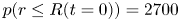$p(r\le R(t=0))=2700$ bar. The effect of the viscosity on the maximum bubble radius $R_{max}$ is rather mild, thus the range of $0.00025\le 1/Re\le 0.027$ covers approximately the viscosity range $10^{-3}\ \textrm {Pa} \cdot \textrm {s} \le \mu \le 0.1 \ \textrm {Pa} \cdot \textrm {s}$.

6.1. Inward shear stress

Let us first look at $\tau _{mn}$ in figure 13$(a)$. In general, the inward stress, $\tau _{mn}$, increases with $1/Re$ while decreases with $\gamma$ monotonically. Here, $\tau _{mn}$ increases faster with $1/Re$ at low $\gamma$ values as compared with higher $\gamma$ values. To understand this dependency of $\tau _{mn}$, we now apply the typical boundary layer analysis (Schlichting & Gersten Reference Schlichting and Gersten2016) to the flow profile of the expanding and collapsing bubble. At any time of the flow, we can estimate the wall shear stress as $\tau \sim \mu U_\infty /\delta$ with the outer radial velocity $U_\infty$ of the boundary layer and the boundary layer thickness $\delta$. Within the boundary layer, the inertia forces balance the friction in the boundary layer, thus in an axisymmetric flow, we can relate

(6.1)\begin{equation} \rho u \partial u/ \partial r \sim\mu\partial^2 u/\partial y^2.\end{equation}

The wall-perpendicular velocity gradient $\partial u/\partial y$ is of order $U_\infty /\delta$, thus relation (6.1) becomes

(6.2)\begin{equation} \rho U_\infty \partial U_\infty/ \partial r \sim \mu U_\infty/\delta^2,\end{equation}

and the thickness of the boundary layer scales as

(6.3)\begin{equation} \delta \sim \left(\frac{\mu}{\rho}\frac{1}{\partial U_\infty/\partial r}\right)^{0.5}.\end{equation}

Then the wall shear stress can be estimated as

(6.4)\begin{equation} \tau \sim (\rho\mu)^{0.5} U_\infty (\partial U_\infty/\partial r)^{0.5}.\end{equation}

For the inward flow, $U_\infty$ decreases with $r$ outside the bubble, therefore the expression $U_\infty (\partial U_\infty /\partial r)^{0.5}$ increases with $U_\infty$. Consequently, for each bubble, the maximum inward stress $\tau _{mn}$ occurs at the maximum velocity $U_{\infty,mn}$ of the inward flow.

To estimate the scaling of the maximum inward wall shear stress with $\gamma$ and $1/Re$, it seems that a knowledge of the maximum of the expression $U_{\infty,mn}(\partial U_{\infty,mn}/\partial r)$ would be necessary. Unfortunately, this expression is difficult to obtain or even estimate. Let us explain why. The magnitude of the inward stress increases during the shrinkage of the bubble. Although the rate of the change of $\tau$ is not strongly dependent on $\gamma$, the instant of time when the increase of the inwards stress ends is determined by $\gamma$. For large stand-off distance, we find that once the jet impacts on the boundary, the flow direction of the liquid near the boundary is abruptly changed from inward to outward, see figures 11$(d)$ and 12$(d)$. As a result, for large $\gamma$ values, the maximum inward shear stress occurs just at the time of jet impact. For a bubble closer to the boundary (small $\gamma$), the liquid underneath the bubble is trapped. The jet impact results in an upwards splash into the bubble and thus prevents the jet from abruptly stopping the inward flow. Hence, the boundary layer for large $r>R(t)$ continues accelerating inwards until the bubble has further collapsed and the vortex ring, which is a result of the upwards lifted jet, spreads out, see figures 8(d,e) and 10(d,e). As a result, the inward shear stress can increase to larger values as it is affected only later by the spreading jet.

Therefore, the maximum velocity $U_{\infty,mn}$ of the inward flow is increasing with decreasing $\gamma$. Let us include the effect of the viscosity by suggesting that $\tau _{mn} \sim f(\mu ^{0.5},\gamma )\sim f((1/Re)^{0.5},\gamma )$. We find that we can collapse the $\tau _{mn}$ values onto a line once we plot $\tau _{mn} Re^{0.35}$ versus $\gamma$ rather than $\tau _{mn} Re^{0.5}$, see figure 14. The expected scaling $\tau _{mn} \sim (1/Re)^{0.5}$ reduces to $\tau _{mn} \sim (1/Re)^{0.35}$ mainly owing to the viscous dissipation of the flow for $0.001\ \textrm {Pa}\cdot \textrm {s} \le \mu \le 0.1\ \textrm {Pa}\cdot \textrm {s}$. The line fitted to the range $0.5<\gamma <1.4$ is $\tau _{mn} Re^{0.35}=-70\gamma +110$(kPa) for $0.01\ \mathrm {Pa}\cdot \textrm {s} \le \mu \le 0.1\ \mathrm {Pa}\cdot \textrm {s}$, while it reduces to $\tau _{mn} Re^{0.35}=-70\gamma +100$(kPa) for $\mu =10^{-3}\ \mathrm {Pa}\cdot \textrm {s}$ mainly owing to a faster bubble motion that reduces the growth time of the shrinking flow in water.

Figure 14. Graph of $\tau _{mn} Re^{0.35}$ versus $\gamma$. The dashed line represents $-70\gamma +110$ (kPa). The doted line is $-70\gamma +100$ (kPa). The symbols indicate liquid with various viscosity.

6.2. Outward shear stress

The distribution of $\tau _{mp}$ reveals a more complex parameter space of $(1/Re,\gamma )$, see figure 13$(b)$. At low $1/Re, \tau _{mp}$ first increases then decreases with $\gamma$; while at high $1/Re, \tau _{mp}$ always decreases with $\gamma$. The two local maxima are located at ($1/Re\approx 0.006, \gamma \approx 1.0$) and ($1/Re\approx 0.026, \gamma \approx 0.5$), and the contour levels reveal that the gradient of the wall shear stress is stronger near the peak at low $1/Re$.

Now we focus on the location where the maximum outward shear occurs and connect its value with the bubble dynamics. Let us take $\tau _{mp}$ occurring at time $t=t_{mp}$ and a distance $r=r_{mp}$. Now at $r=r_{mp}$, the maximum radial velocity along the $y$ direction is considered as the outer velocity of the boundary layer $U_{\infty,mp}$. Next we will use $U_{\infty,mp}$ as an intermediate variable to connect $\tau _{mp}$ with $U_{jet}, h_{jet}$ and the liquid viscosity $\mu$. For a further step, we can rewrite (6.3) for the boundary layer thickness as

(6.5)\begin{equation} \delta_{mp} \sim \left(\frac{\mu}{\rho}\frac{1}{\partial U_{\infty/,mp}\partial r}\right)^{0.5}= \mu^{0.5} \rho^{{-}0.5} U_{\infty,mp}^{{-}0.5} l_m^{\,0.5},\end{equation}

where $l_m={U_{\infty,mp}}/{\partial U_{\infty,mp}/\partial r}$ is a characteristic length for the spreading flow growing from zero to the outer velocity, which is a non-trivial function that is dependent on the bubble shape.

While tempting, the analytic similarity solution $\tau \sim r ^{-11/4}$ for the steady Glauert jet (Glauert Reference Glauert1956) is not applicable to estimate the maximum wall shear stress of the present transient and finite-sized jets. Yet it predicts, even for a steady jet, a rapid decrease of the wall shear stress with distance $r$. If we neglect the bubble deformation after jet impact, a reasonable estimate of the location where the maximum outward stress occurs is at the edge of the impinging jet $r=R_{jet}$ (see figures 8–12$d$). This radius $R_{jet}\propto R_{max}$ increases linearly with maximum radius of the bubble (see figure 6$(c)$, where $R_{jet}/R_{max} \approx 0.3$). Assuming conservation of mass for the incompressible impinging jet, we have $\rho U_{jet} R_{jet}^2 =\rho U_{\infty,mp} 2R_{jet}h_{jet}$ at $r=R_{jet}$, thus $U_{\infty,mp}/U_{jet} \sim R_{max}/h_{jet}$. However, this expression is incomplete as the bubble deformation is involved and viscosity contributes through energy dissipation in the unsteady boundary layer. Therefore we use two exponents $\alpha$ and $\beta$ that account for the geometric and viscous effects with

(6.6)\begin{equation} \frac{U_{\infty,mp}}{U_{jet}} \sim \left(\frac{R_{max}}{h_{jet}}\right)^\alpha Re^\beta. \end{equation}

Next we determine the values of $\alpha$ and $\beta$ based on our computed results. Figure 15 plots the various combinations of $Re$ and $U_{\infty,mp}/U_{jet}$ as a function of $R_{max}/h_{jet}$ in a log–log plot. Note that the opacity of the plotted data indicates the $\gamma$ value from low to high with light to dark. Figure 15 shows that the values of $\alpha$ and $\beta$ are not constant but vary with $\gamma$. The shape reveals, as expected, two regimes with different scaling, namely for small and large $\gamma$. By fitting lines to the data in figure 15 , we obtain $(\alpha,\beta )=(0.2,0.2)$ for $\gamma \leq 1.1$ and $(\alpha,\beta )=(1.0,0.5)$ for $\gamma \geq 1.1$. Combining (6.5) and (6.6) into $\tau _{s,mp} \sim \mu U_{\infty,mp}/\delta _{mp}$, we obtain

(6.7)\begin{equation} \tau_{s,mp} \sim \mu^{0.2} h_{jet}^{{-}0.3} U_{jet}^{1.5} l_m^{{-}0.5},\end{equation}

for $\gamma \leq 1.1$, and

(6.8)\begin{equation} \tau_{s,mp} \sim \mu^{{-}0.25} h_{jet}^{{-}1.5} U_{jet}^{1.5} l_m^{{-}0.5},\end{equation}

for $\gamma \geq 1.1$, where $\tau _{s,mp}$ denotes the maximum outward stress from the above scaling law. The above laws can be written in a dimensionless form:

(6.9)\begin{equation} \bar{\tau}_{s,mp} \sim Re^{{-}0.2} \bar{h}_{jet}^{{-}0.3} \bar{U}_{jet}^{1.5} \bar{l}_m^{{-}0.5}, \end{equation}

for $\gamma \leq 1.1$, and

(6.10)\begin{equation} \bar{\tau}_{s,mp} \sim Re^{0.25} \bar{h}_{jet}^{{-}1.5} \bar{U}_{jet}^{1.5} \bar{l}_m^{{-}0.5}, \end{equation}

for $\gamma \geq 1.1$, where $\bar {\tau }_{s,mp}=\tau _{s,mp}/P_\infty, \bar {h}_{jet}= h_{jet}/R_{max}, \bar {U}_{jet}= U_{jet}/U_0$ and $\bar {l}_m = l_m/R_{max}$.

Figure 15. The log–log plot for (6.6). The slopes of dashed lines are 0.2 in panel $(a)$ and 1.0 in panel $(b)$. The $\gamma$ values from 0.5 to 1.6 for each viscosity are indicated by the opacity of the symbols from light to dark. Note the $y$-axis variables are different in the two plots: $(a)$ data of small $\gamma$ (light opacity) collapse with a slope of 0.2; $(b)$ data of large $\gamma$ (dark opacity) collapse with a slope of 1.0.

To examine the scaling, we need information of the gap thickness $\bar {h}_{jet}$ and the jet velocity $\bar {U}_{jet}$ while considering $\bar {l}_m$ has a small effect. The results are reported in § 4 figure 7. Next we insert in the relations (6.9) and (6.10) the $\bar {h}_{jet}$ and $\bar {U}_{jet}$ from the simulations shown in figure 7a,b to obtain $\bar {\tau }_{s,mp}$. How does this value compare with $\tau _{mp}$? Figure 16$(a)$ combines both $\bar {\tau }_{s,mp}$ from relations (6.7) and (6.8) in one plot; note that the plotted variable $\tau ^{*}_{s,mp}$ is the result of $\bar {\tau }_{s,mp}$ normalized by its maximum value.

Figure 16. $(a)$ Distribution of $\tau ^*_{s,mp}$ on ($1/Re, \gamma$), where $\tau ^*_{s,mp}$ is the wall shear stress calculated by (6.9) and (6.10) with the input of $\bar {h}_{jet}$ and $\bar {U}_{jet}$ from figure 7 and normalized by its maximum value. $(b)$ Comparison of the result using the scaling laws and the simulation result $\tau _{mp}^*$, which is a normalized value of $\tau _{mp}$ by its maximum value. The dashed line represents $\tau ^*=\tau _{mp}^*$.

The landscape of $\tau ^*_{s,mp}(1/Re,\gamma )$ shares similar features as $\tau _{mp}(1/Re,\gamma )$ in figure 13$(b)$ with both local maximum values occurring at almost the same locations. For comparison, we plot $\tau ^*_{s,mp}$ against the normalized $\tau _{mp}, \tau _{mp}^{*}$, in figure 16$(b)$ and we find, overall, a linear relationship. Yet there are deviations that are caused by the richness of the flow field and resulting bubble shapes briefly before the bubble collapse. For example, we observe a splitting of the main bubble resulting in daughter toroidal bubbles close to the boundary for $\gamma >1.0$ (see small red arrow in figure 11$e$). It is expected that these flows alter notably the wall shear stress by affecting the characteristic length $l_m$ in (6.7) and (6.8). These complex shapes are relevant and seen in experiments, e.g. by Brujan et al. (Reference Brujan, Keen, Vogel and Blake2002), Zhang et al. (Reference Zhang, Li and Cui2015). Overall, the scaling of relations (6.9) and (6.10) capture the dependence of the maximum stress as a function of viscosity, $\mu$, gap thickness, $h_{jet}$, and jet velocity, $U_{jet}$.