


1. Introduction
Roughness plays an important role in the fluid dynamics of numerous transport processes. Most surfaces in engineering applications are rough and, as a consequence, rough-wall turbulent flows have also been studied by many investigators. A major difference between smooth- and rough-wall flows is that for smooth walls, there is only viscous drag, while for rough-wall flows, both pressure (form) drag and viscous drag exist. In a smooth-wall pipe or channel flow, there is only a favourable mean pressure gradient. However, for pipe or channel flows having sufficiently organized roughness, there can be spatially localized regions in which an adverse mean pressure gradient persists, as seen, for example, in the region upstream of spanwise rib roughness, e.g. Leonardi et al. (Reference Leonardi, Orlandi, Smalley, Djenidi and Antonia2003).
Hydraulic pipes or channels are often designed with different wall geometries in order to accommodate specific design objectives, such as industrial and compact heat exchangers, blood oxygenators in extra-corporeal systems, membrane separators, vortex wave membrane bioreactors, etc. One of the popular forms is a wavy shape. Two common configurations in wavy passages have been reported in several investigations. One is a pipe or channel with periodically converging–diverging cross-section where the flow axis is straight. The other is a pipe or channel with uniform cross-section but with a wavy flow axis. These two configurations are usually referred to as symmetric and asymmetric flow passages respectively. Symmetric wavy flow passages can take the form of different geometries such as triangular (Sparrow & Prata Reference Sparrow and Prata1983; Faghri & Asako Reference Faghri and Asako1987; Hossain & Islam Reference Hossain and Islam2004; Eiamsa-ard & Promvonge Reference Eiamsa-ard and Promvonge2007), arc shaped (Tatsuo et al. Reference Tatsuo, Shinichiro, Shingho and Yuji1990; Bahaidarah, Anand & Chen Reference Bahaidarah, Anand and Chen2005) or an ‘egg-carton’ shape (Sawyers, Sen & Chang Reference Sawyers, Sen and Chang1998). Asymmetric wavy passages with uniform cross-section commonly have either zigzag (O’Brien Reference O’Brien1982; Asako & Faghri Reference Asako and Faghri1987; Faghri & Asako Reference Faghri and Asako1987; Hwang, Jang & Cho Reference Hwang, Jang and Cho2006) or sinusoidal flow axes (Popiel & Van der Merwe Reference Popiel and Van der Merwe1996; Wang & Du Reference Wang and Du2008; Guzmán et al. Reference Guzmán, Cárdenas, Urzúa and Araya2009; Sui, Teo & Lee Reference Sui, Teo and Lee2012). In addition, different types of spiral shapes (another kind of waviness) are commonly used for promoting mixing, e.g. helical pipes (Cookson, Doorly & Sherwin Reference Cookson, Doorly and Sherwin2009). However, an asymmetric pipe with a sinusoidal flow axis provides more vigorous mixing through the alternating bends than, for example, in coiled pipes (Shimizu et al. Reference Shimizu, Sugino, Kuzuhara and Murakami1982).
Various linear stability analyses have been presented of incompressible flows in corrugated channels and pipes. It is accepted that laminar flow in straight pipes is linearly stable at all Reynolds numbers investigated to date. The two studies most relevant to the present work are those by Cotrell, MacFadden & Alder (Reference Cotrell, MacFadden and Alder2008) and Loh & Blackburn (Reference Loh and Blackburn2011), which both analysed flows in axisymmetrically corrugated pipes. Cotrell et al. (Reference Cotrell, MacFadden and Alder2008) mainly analysed axisymmetric instability for axis wavelengths incommensurate with the corrugation wavelength
 $L_{m}=0.5D$
and showed that the addition of corrugation makes the laminar flow unstable to axisymmetric disturbances, although, for the corrugation amplitudes employed in the present work, at rather large Reynolds numbers. Loh & Blackburn (Reference Loh and Blackburn2011) concentrated instead on three-dimensional disturbances in wavy-wall pipes at the same corrugation wavelength of
$L_{m}=0.5D$
and showed that the addition of corrugation makes the laminar flow unstable to axisymmetric disturbances, although, for the corrugation amplitudes employed in the present work, at rather large Reynolds numbers. Loh & Blackburn (Reference Loh and Blackburn2011) concentrated instead on three-dimensional disturbances in wavy-wall pipes at the same corrugation wavelength of
 $L_{m}=0.5D$
employed by Cotrell et al. (Reference Cotrell, MacFadden and Alder2008) and demonstrated that the laminar flow became unstable to disturbances of low azimuthal wavenumber
$L_{m}=0.5D$
employed by Cotrell et al. (Reference Cotrell, MacFadden and Alder2008) and demonstrated that the laminar flow became unstable to disturbances of low azimuthal wavenumber
 $k_{o}=3$
, 4 at Reynolds numbers of order 2000–3000 for comparatively small corrugation amplitudes. We will return to consideration of these findings in relation to our results in §§ 4 and 6.
$k_{o}=3$
, 4 at Reynolds numbers of order 2000–3000 for comparatively small corrugation amplitudes. We will return to consideration of these findings in relation to our results in §§ 4 and 6.
Direct numerical simulations (DNS) of turbulent flow for wavy walls and walls with transverse ribs have been carried out by many researchers; in part to gain a deeper understanding of rough-wall turbulent flows. These geometries are commonly accepted as idealizations of ‘rough-wall’ turbulent flows. To date, however, DNS of turbulent fluid flow in symmetric wavy-wall pipes is relatively limited, although some related studies have been conducted which consider asymmetric wavy pipe or channel flows. The present effort on symmetric wavy-wall pipes builds upon the initial study of Blackburn, Ooi & Chong (Reference Blackburn, Ooi and Chong2007). The most recent DNS of fluid flow and heat transfer in asymmetric sinusoidal wavy channels were performed by Guzmán et al. (Reference Guzmán, Cárdenas, Urzúa and Araya2009) and Sui et al. (Reference Sui, Teo and Lee2012). These investigations were, however, limited to the laminar and transitional regimes. Wang & Du (Reference Wang and Du2008) carried out DNS studies of viscous flow in a pipe having asymmetric sinusoidal wall corrugations for a friction Reynolds number
 $\mathit{Re}_{{\it\tau}}$
of up to 670.
$\mathit{Re}_{{\it\tau}}$
of up to 670.
A knowledge of the scaling properties of turbulent flow for the cases of smooth, transitionally rough and fully rough pipe or channel flows is important to the design of many commercial applications. The roughness height of a surface,
 $k$
, was considered by Nikuradse (Reference Nikuradse1933) to usefully characterize the roughness-induced properties of the mean profile. The concept of ‘equivalent sand-grain roughness’,
$k$
, was considered by Nikuradse (Reference Nikuradse1933) to usefully characterize the roughness-induced properties of the mean profile. The concept of ‘equivalent sand-grain roughness’,
 $k_{s}$
, was discussed in Nikuradse (Reference Nikuradse1933) and Schlichting (Reference Schlichting1936), and is commonly used by engineers to classify the so-called fully smooth, fully rough or transitionally rough conditions. This classification has been employed in numerous studies (e.g. Jimenez Reference Jimenez2004; Gioia, Chakraborty & Bombardelli Reference Gioia, Chakraborty and Bombardelli2006; Shockling, Allen & Smits Reference Shockling, Allen and Smits2006; Allen, Shockling, Kunkel & Smits Reference Allen, Shockling, Kunkel and Smits2007; Flack & Schultz Reference Flack and Schultz2010). More recently, Mehdi, Klewicki & White (Reference Mehdi, Klewicki and White2013) provided evidence that, because of the combined dependences on roughness and Reynolds number, there exists a richer set of dynamically distinct roughness regimes than indicated by the traditional classification. In general, these regimes become more apparent as the overall scale separation (friction Reynolds number) becomes large.
$k_{s}$
, was discussed in Nikuradse (Reference Nikuradse1933) and Schlichting (Reference Schlichting1936), and is commonly used by engineers to classify the so-called fully smooth, fully rough or transitionally rough conditions. This classification has been employed in numerous studies (e.g. Jimenez Reference Jimenez2004; Gioia, Chakraborty & Bombardelli Reference Gioia, Chakraborty and Bombardelli2006; Shockling, Allen & Smits Reference Shockling, Allen and Smits2006; Allen, Shockling, Kunkel & Smits Reference Allen, Shockling, Kunkel and Smits2007; Flack & Schultz Reference Flack and Schultz2010). More recently, Mehdi, Klewicki & White (Reference Mehdi, Klewicki and White2013) provided evidence that, because of the combined dependences on roughness and Reynolds number, there exists a richer set of dynamically distinct roughness regimes than indicated by the traditional classification. In general, these regimes become more apparent as the overall scale separation (friction Reynolds number) becomes large.
The highly regular form of roughness considered in the present investigation is not typical of many practical applications. It does, however, afford opportunities to theoretically relate various important parameters, like the pressure drop and friction factor, to the roughness topography. This is contrasted with the classical view of Nikuradse (Reference Nikuradse1933) and Schlichting (Reference Schlichting1936) which, at least partially, supports a broad framework for roughness scalings based upon the notion of equivalent sand-grain roughness. Consider, for example, a fully developed pipe flow having a small but dimensionally fixed roughness. At a low Reynolds number, when normalized equivalent sand-grain roughness
 $k_{s}^{+}=k_{s}u_{{\it\tau}}/{\it\nu}$
is small, the flow is hydraulically smooth and there is no detectable effect of roughness. With an increase in the Reynolds number, the flow becomes transitionally rough. Here, the friction factor is higher than in smooth-wall flow, and is a function of both the roughness height and the Reynolds number. Further increase in the Reynolds number forces the flow to become fully rough. Here,
$k_{s}^{+}=k_{s}u_{{\it\tau}}/{\it\nu}$
is small, the flow is hydraulically smooth and there is no detectable effect of roughness. With an increase in the Reynolds number, the flow becomes transitionally rough. Here, the friction factor is higher than in smooth-wall flow, and is a function of both the roughness height and the Reynolds number. Further increase in the Reynolds number forces the flow to become fully rough. Here,
 $k_{s}^{+}$
is large, and the friction factor essentially loses its dependence on the Reynolds number.
$k_{s}^{+}$
is large, and the friction factor essentially loses its dependence on the Reynolds number.
The two-layer theory of Millikan (Reference Millikan, den Hartog and Peters1938) has been applied to the transitionally rough and fully rough regimes. In accord with observations, this theory provides for a formulation of the mean velocity profile that accounts for an additive constant that depends on the roughness length scale. All traditional rough-wall scaling theories are based on either the smooth-wall variable,
 $y^{+}$
, or the rough-wall variable,
$y^{+}$
, or the rough-wall variable,
 $y/k$
, as considered by Benedict (Reference Benedict1980), Raupach, Antonia & Rajagopalan (Reference Raupach, Antonia and Rajagopalan1991), Jimenez (Reference Jimenez2004) and many others. In this case, the additive constant in the logarithmic mean profile formula is supplemented with the roughness function,
$y/k$
, as considered by Benedict (Reference Benedict1980), Raupach, Antonia & Rajagopalan (Reference Raupach, Antonia and Rajagopalan1991), Jimenez (Reference Jimenez2004) and many others. In this case, the additive constant in the logarithmic mean profile formula is supplemented with the roughness function,
 ${\rm\Delta}U^{+}$
, as proposed by Clauser (Reference Clauser1954) and Hama (Reference Hama1954). Physically,
${\rm\Delta}U^{+}$
, as proposed by Clauser (Reference Clauser1954) and Hama (Reference Hama1954). Physically,
 ${\rm\Delta}U^{+}$
represents a loss of mean momentum relative to the smooth-wall flow, as it generally describes an increasing downward shift in the mean velocity profile with increasing roughness (due to an increasing drag force). Hence, a number of methods have been explored to determine the roughness function
${\rm\Delta}U^{+}$
represents a loss of mean momentum relative to the smooth-wall flow, as it generally describes an increasing downward shift in the mean velocity profile with increasing roughness (due to an increasing drag force). Hence, a number of methods have been explored to determine the roughness function
 ${\rm\Delta}U^{+}$
(Granville Reference Granville1987; Schultz & Myers Reference Schultz and Myers2003).
${\rm\Delta}U^{+}$
(Granville Reference Granville1987; Schultz & Myers Reference Schultz and Myers2003).
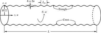
Figure 1. Schematic view of the simulation domain for the wavy-wall pipe along with the cylindrical-coordinate system.
Townsend (Reference Townsend1956) observed that for
 $k/D\ll 1$
the profiles of
$k/D\ll 1$
the profiles of
 $U^{+}$
and
$U^{+}$
and
 $\langle u^{\prime }\rangle ^{+}$
, when plotted versus the outer-normalized distance from the wall, do not exhibit a dependence on the surface roughness. He hypothesized that the influence of roughness at high Reynolds number was only localized in a region where the roughness scales directly influenced the scales of the turbulence. This wall-similarity hypothesis has been shown to at least approximately hold for a variety of roughness topographies, including cylindrical roughness, sand-grain, mesh, spheres and two-dimensional grooves (Flack, Schultz & Shapiro Reference Flack, Schultz and Shapiro2005). There are also notable cases, such as two-dimensional bars, where this hypothesis apparently fails to hold, e.g. see Mehdi et al. (Reference Mehdi, Klewicki and White2013). Recently, Chung, Monty & Ooi (Reference Chung, Monty and Ooi2014) presented an idealized assessment of Townsend’s outer-layer similarity hypothesis by using uniform shear-stress boundary conditions. Their results suggested that wall-turbulence motions of energetic significance obtained their character from the wall shear stress and wall impermeability. All these considerations motivate the exploration of how the present corrugation height influences outer-layer similarity.
$\langle u^{\prime }\rangle ^{+}$
, when plotted versus the outer-normalized distance from the wall, do not exhibit a dependence on the surface roughness. He hypothesized that the influence of roughness at high Reynolds number was only localized in a region where the roughness scales directly influenced the scales of the turbulence. This wall-similarity hypothesis has been shown to at least approximately hold for a variety of roughness topographies, including cylindrical roughness, sand-grain, mesh, spheres and two-dimensional grooves (Flack, Schultz & Shapiro Reference Flack, Schultz and Shapiro2005). There are also notable cases, such as two-dimensional bars, where this hypothesis apparently fails to hold, e.g. see Mehdi et al. (Reference Mehdi, Klewicki and White2013). Recently, Chung, Monty & Ooi (Reference Chung, Monty and Ooi2014) presented an idealized assessment of Townsend’s outer-layer similarity hypothesis by using uniform shear-stress boundary conditions. Their results suggested that wall-turbulence motions of energetic significance obtained their character from the wall shear stress and wall impermeability. All these considerations motivate the exploration of how the present corrugation height influences outer-layer similarity.
Afzal & Seena (Reference Afzal and Seena2007), Afzal (Reference Afzal2013) and Afzal, Seena & Bushra (Reference Afzal, Seena and Bushra2013) recently proposed roughness scaling laws for transitionally rough pipes which employ alternate variables. They defined an inner transitional roughness variable as the ratio of the wall-normal coordinate measured above the mean roughness level to the actual wall roughness level. They provided evidence that this allows one to express the mean velocity profile and friction factor in a universal form for the transitionally rough flows that they considered. Similarly, using the same alternate variables Afzal, Seena & Bushra (Reference Afzal, Seena and Bushra2006) also proposed an alternate power-law velocity profile for transitionally rough pipe flows. These same authors also developed expressions for the scaling properties of an intermediate layer in a transitionally rough channel flow (Seena & Afzal Reference Seena and Afzal2008). By proposing a matched asymptotic expansion solution, they showed evidence of an intermediate layer having its own characteristic scaling and existing between the traditional inner and outer layers. Herein, we explore the validity of intermediate variables that arise by directly considering invariant forms admitted by mean momentum equation.
In the present work we study DNS of incompressible flows within straight pipes whose walls have smooth sinusoidal corrugations, e.g. as shown in figure 1. The corrugation wavelength is maintained constant and the amplitude of the wave is varied, thus allowing a straightforward parametric variation of the corrugation height. At any Reynolds number, this means that the wavelength is constant with respect to streamwise length scales of flow in a smooth pipe. We note, however, that the corrugations so generated are not geometrically self-similar. We investigate variations of both the wave height and the Reynolds number. The present Reynolds number range spans from the laminar regime, through the transitional regime and into the low-Reynolds-number turbulent regime. Our analysis focuses on examining the effect of variations in
 $h/D$
, where
$h/D$
, where
 $h$
is the peak-to-peak wave height at a fixed
$h$
is the peak-to-peak wave height at a fixed
 $\mathit{Re}_{{\it\tau}}$
while allowing the bulk-flow Reynolds number,
$\mathit{Re}_{{\it\tau}}$
while allowing the bulk-flow Reynolds number,
 $\mathit{Re}_{D}$
, to vary. The outcomes are not readily extended to cover the effect of variations of
$\mathit{Re}_{D}$
, to vary. The outcomes are not readily extended to cover the effect of variations of
 $h/D$
at fixed
$h/D$
at fixed
 $\mathit{Re}_{D}$
.
$\mathit{Re}_{D}$
.
2. Mathematical formulation
2.1. Problem definition
The dynamics of the flow is established by the incompressible Navier–Stokes equations,
 $$\begin{eqnarray}\displaystyle & \partial _{t}\boldsymbol{u}+\boldsymbol{N}(\boldsymbol{u})=-{\it\rho}^{-1}\boldsymbol{{\rm\nabla}}p+{\it\nu}{\rm\nabla}^{2}\boldsymbol{u}+\boldsymbol{g}, & \displaystyle\end{eqnarray}$$
 $$\begin{eqnarray}\displaystyle & \boldsymbol{{\rm\nabla}}\boldsymbol{\cdot }\boldsymbol{u}=0, & \displaystyle\end{eqnarray}$$
 $p$
is the fluctuating pressure,
$p$
is the fluctuating pressure,
 ${\it\rho}$
is the density of the fluid,
${\it\rho}$
is the density of the fluid,
 ${\it\nu}$
is the kinematic viscosity,
${\it\nu}$
is the kinematic viscosity,
 $\boldsymbol{g}$
is a forcing vector and
$\boldsymbol{g}$
is a forcing vector and
 $\boldsymbol{N}(\boldsymbol{u})$
represents the nonlinear advection terms. Since a wavy-wall pipe is axisymmetric, it is convenient to examine the problem in a cylindrical-coordinate system, and thus we denote the axial, radial and azimuthal components of velocity by
$\boldsymbol{N}(\boldsymbol{u})$
represents the nonlinear advection terms. Since a wavy-wall pipe is axisymmetric, it is convenient to examine the problem in a cylindrical-coordinate system, and thus we denote the axial, radial and azimuthal components of velocity by
 $\boldsymbol{u}(z,r,{\it\theta})(t)=(u,v,w)(t)$
. For a fully developed turbulent pipe flow the driving force
$\boldsymbol{u}(z,r,{\it\theta})(t)=(u,v,w)(t)$
. For a fully developed turbulent pipe flow the driving force
 $\boldsymbol{g}=(g,0,0)$
corresponds to the mean pressure gradient in the streamwise
$\boldsymbol{g}=(g,0,0)$
corresponds to the mean pressure gradient in the streamwise
 $z$
direction, and, as is common in simulations of this type, is used in order to allow both the pressure and the velocity to be axially periodic. No-slip boundary conditions are applied to the velocity field along the walls of the domain.
$z$
direction, and, as is common in simulations of this type, is used in order to allow both the pressure and the velocity to be axially periodic. No-slip boundary conditions are applied to the velocity field along the walls of the domain.
The fundamental length scale is the diameter
 $D$
of the corresponding smooth pipe. The highest Kármán number or friction Reynolds number is
$D$
of the corresponding smooth pipe. The highest Kármán number or friction Reynolds number is
 $\mathit{Re}_{{\it\tau}}=u_{{\it\tau}}D/2{\it\nu}=314$
. Here, the friction velocity is defined by
$\mathit{Re}_{{\it\tau}}=u_{{\it\tau}}D/2{\it\nu}=314$
. Here, the friction velocity is defined by
 $u_{{\it\tau}}=({\it\tau}_{o}/{\it\rho})^{1/2}$
, where
$u_{{\it\tau}}=({\it\tau}_{o}/{\it\rho})^{1/2}$
, where
 ${\it\tau}_{o}$
is the mean wall shear stress. The axial mean pressure gradient per unit mass
${\it\tau}_{o}$
is the mean wall shear stress. The axial mean pressure gradient per unit mass
 $g_{o}=4{\it\tau}_{o}/{\it\rho}D={\it\lambda}{\it\rho}U_{b}^{2}/2D$
(where
$g_{o}=4{\it\tau}_{o}/{\it\rho}D={\it\lambda}{\it\rho}U_{b}^{2}/2D$
(where
 $U_{b}$
is the bulk-flow velocity) is required to drive the flow in a smooth pipe, and the friction factor
$U_{b}$
is the bulk-flow velocity) is required to drive the flow in a smooth pipe, and the friction factor
 ${\it\lambda}$
in smooth pipes is given by
${\it\lambda}$
in smooth pipes is given by
 $$\begin{eqnarray}{\it\lambda}=8{\it\tau}_{o}/({\it\rho}U_{b}^{2}).\end{eqnarray}$$
Here,
 $U_{b}$
is used to define the bulk-flow Reynolds number as
$U_{b}$
is used to define the bulk-flow Reynolds number as
 $\mathit{Re}_{D}=U_{b}D/{\it\nu}=4\langle Q\rangle /{\rm\pi}D{\it\nu}$
, where
$\mathit{Re}_{D}=U_{b}D/{\it\nu}=4\langle Q\rangle /{\rm\pi}D{\it\nu}$
, where
 $\langle Q\rangle$
is the average volumetric flow rate. From the definitions above one can also determine that
$\langle Q\rangle$
is the average volumetric flow rate. From the definitions above one can also determine that
 $$\begin{eqnarray}{\it\lambda}=32(\mathit{Re}_{{\it\tau}}/\mathit{Re}_{D})^{2}.\end{eqnarray}$$
The methodology pursued in the present work produces sets of simulations, each with constant
 $\mathit{Re}_{{\it\tau}}$
, from the maximum value
$\mathit{Re}_{{\it\tau}}$
, from the maximum value
 $\mathit{Re}_{{\it\tau}}=314$
down to the laminar regime, typically with the driving force per unit mass
$\mathit{Re}_{{\it\tau}}=314$
down to the laminar regime, typically with the driving force per unit mass
 $g_{o}$
halved between successive sets. Since
$g_{o}$
halved between successive sets. Since
 $$\begin{eqnarray}\mathit{Re}_{{\it\tau}}=(g_{o}D^{3}/16{\it\nu}^{2})^{1/2},\end{eqnarray}$$
the friction Reynolds number typically varies by a factor of
 $(2)^{-1/2}$
between successive sets of simulations. It should be noted that the Blasius friction factor correlation for smooth pipes is given by
$(2)^{-1/2}$
between successive sets of simulations. It should be noted that the Blasius friction factor correlation for smooth pipes is given by
 ${\it\lambda}=0.3164\mathit{Re}_{D}^{-1/4}$
(Nikuradse Reference Nikuradse1933); for moderate turbulent Reynolds numbers this yields the relationship
${\it\lambda}=0.3164\mathit{Re}_{D}^{-1/4}$
(Nikuradse Reference Nikuradse1933); for moderate turbulent Reynolds numbers this yields the relationship
 $\mathit{Re}_{{\it\tau}}=0.09944\mathit{Re}_{D}^{7/8}$
. Consequently, the maximum value of the bulk-flow Reynolds number in the smooth pipe for the present work, with
$\mathit{Re}_{{\it\tau}}=0.09944\mathit{Re}_{D}^{7/8}$
. Consequently, the maximum value of the bulk-flow Reynolds number in the smooth pipe for the present work, with
 $\mathit{Re}_{{\it\tau}}=314$
, is
$\mathit{Re}_{{\it\tau}}=314$
, is
 $\mathit{Re}_{D}\approx 10\,000$
.
$\mathit{Re}_{D}\approx 10\,000$
.
All the domains have the same mean radius
 $\bar{R}=D/2$
, and for turbulent flow calculations the same axial length
$\bar{R}=D/2$
, and for turbulent flow calculations the same axial length
 $L=2{\rm\pi}D$
. The length to diameter ratio was chosen based on the previous pipe length convergence studies by Chin et al. (Reference Chin, Ooi, Marusic and Blackburn2010). They showed that a pipe length of at least
$L=2{\rm\pi}D$
. The length to diameter ratio was chosen based on the previous pipe length convergence studies by Chin et al. (Reference Chin, Ooi, Marusic and Blackburn2010). They showed that a pipe length of at least
 $2{\rm\pi}D$
is required to achieve converged turbulent-flow statistics for
$2{\rm\pi}D$
is required to achieve converged turbulent-flow statistics for
 $\mathit{Re}_{{\it\tau}}\approx 500$
.
$\mathit{Re}_{{\it\tau}}\approx 500$
.
For the wavy-wall flows, 15 corrugation wavelengths were chosen within the domain length of
 $2{\rm\pi}D$
. This number is large enough to ensure that, even at transitional Reynolds numbers, the number of wavelengths is sufficient to reduce the streamwise correlation of near-wall structures to acceptably low values at half the domain length (Chin et al.
Reference Chin, Ooi, Marusic and Blackburn2010). With a corrugation amplitude of
$2{\rm\pi}D$
. This number is large enough to ensure that, even at transitional Reynolds numbers, the number of wavelengths is sufficient to reduce the streamwise correlation of near-wall structures to acceptably low values at half the domain length (Chin et al.
Reference Chin, Ooi, Marusic and Blackburn2010). With a corrugation amplitude of
 $a=h/2$
, the radius of the wavy pipe,
$a=h/2$
, the radius of the wavy pipe,
 $R(z)$
, is given by
$R(z)$
, is given by
 $$\begin{eqnarray}R(z)/D=(\bar{R}/D)+(a/D)\cos (15z/D),\end{eqnarray}$$
as illustrated in figure 1. For laminar-flow calculations, only a single module of the axial wave is represented, i.e. the domain length is reduced to
 $L_{m}=2{\rm\pi}D/15\approx 0.41888D$
.
$L_{m}=2{\rm\pi}D/15\approx 0.41888D$
.
When attempting to define both the bulk-flow and friction Reynolds numbers for a wavy-wall (or any non-uniform) pipe, one needs an equivalent diameter. For simplicity, we have adopted the mean diameter
 $D=2\bar{R}$
for this measure. However, for a constant mean radius the volume of the domain increases as the corrugation height increases, and thus we reduce the driving force
$D=2\bar{R}$
for this measure. However, for a constant mean radius the volume of the domain increases as the corrugation height increases, and thus we reduce the driving force
 $g$
as
$g$
as
 $h$
increases in order to maintain the total body force constant at each
$h$
increases in order to maintain the total body force constant at each
 $\mathit{Re}_{{\it\tau}}$
.
$\mathit{Re}_{{\it\tau}}$
.
From Pappus’ second theorem (Kern & Bland Reference Kern and Bland1948), the domain volume can be found in closed form as
 ${\rm\pi}(\bar{R}^{2}+h^{2}/8)L$
, provided that the length comprises an integral number of wavelengths. Using the equivalent diameter, an equivalent mean wall shear stress is found by equating the mean wall tractive force to the mean body force on the domain, i.e.
${\rm\pi}(\bar{R}^{2}+h^{2}/8)L$
, provided that the length comprises an integral number of wavelengths. Using the equivalent diameter, an equivalent mean wall shear stress is found by equating the mean wall tractive force to the mean body force on the domain, i.e.
 $$\begin{eqnarray}2{\rm\pi}L\bar{R}{\it\tau}_{o}={\it\rho}{\rm\pi}(\bar{R}^{2}+h^{2}/8)Lg,\end{eqnarray}$$
from which
 $$\begin{eqnarray}u_{{\it\tau}}^{2}=\frac{{\it\tau}_{o}}{{\it\rho}}=\frac{\bar{R}}{2}\left(1+\frac{h^{2}}{8\bar{R}^{2}}\right)g.\end{eqnarray}$$
Thus, if one wishes to keep the friction velocity and hence
 $\mathit{Re}_{{\it\tau}}$
constant as
$\mathit{Re}_{{\it\tau}}$
constant as
 $h$
increases, the driving force per unit mass
$h$
increases, the driving force per unit mass
 $g$
must be reduced as
$g$
must be reduced as
 $h$
increases according to
$h$
increases according to
 $$\begin{eqnarray}g(h)=g_{o}V_{o}/V=g_{o}/(1+h^{2}/8\bar{R}^{2}).\end{eqnarray}$$
Here,
 $V_{o}$
is the volume of the smooth-wall pipe and
$V_{o}$
is the volume of the smooth-wall pipe and
 $g_{o}$
is the corresponding axial driving force.
$g_{o}$
is the corresponding axial driving force.
By employing
 $u_{{\it\tau}}$
and
$u_{{\it\tau}}$
and
 $D$
for normalization, equation (2.1) takes on the dimensionless form
$D$
for normalization, equation (2.1) takes on the dimensionless form
 $$\begin{eqnarray}\partial _{{\it\tau}}\boldsymbol{u}^{+}+\boldsymbol{N}(\boldsymbol{u}^{+})=-\boldsymbol{{\rm\nabla}}p^{+}+\frac{1}{2\mathit{Re}_{{\it\tau}}}{\rm\nabla}^{2}\boldsymbol{u}^{+}+\boldsymbol{F}^{+},\end{eqnarray}$$
where
 $\boldsymbol{F}^{+}=(4V_{o}/V,0,0)$
and the ‘
$\boldsymbol{F}^{+}=(4V_{o}/V,0,0)$
and the ‘
 $+$
’ superscript indicates normalization by
$+$
’ superscript indicates normalization by
 ${\it\nu}$
and
${\it\nu}$
and
 $u_{{\it\tau}}$
. The use of (2.9) is well-suited for numerical simulation, as one only needs to assign the value of
$u_{{\it\tau}}$
. The use of (2.9) is well-suited for numerical simulation, as one only needs to assign the value of
 $\mathit{Re}_{{\it\tau}}$
. The resultant value of
$\mathit{Re}_{{\it\tau}}$
. The resultant value of
 $\mathit{Re}_{D}$
can be easily evaluated after the flow field becomes statistically stationary.
$\mathit{Re}_{D}$
can be easily evaluated after the flow field becomes statistically stationary.
Napoli, Armenio & De Marchis (Reference Napoli, Armenio and De Marchis2008) introduced an important roughness parameter called the ‘effective slope’ (ES). The effective slope ES accounts for the roughness corrugation shape, and is defined by
 $$\begin{eqnarray}\mathit{ES}=\frac{1}{L}\int _{L}\left|\frac{\partial R}{\partial z}\right|\,\text{d}z,\end{eqnarray}$$
where, in the present case,
 $L$
is an integral number of corrugations. This function will allow us to investigate the influence of a rough wall on the roughness function as well as friction and pressure drag.
$L$
is an integral number of corrugations. This function will allow us to investigate the influence of a rough wall on the roughness function as well as friction and pressure drag.
Table 1 summarizes the main parameters of the wavy-wall geometries. The maximum peak-to-peak corrugation amplitude of
 $h/D=0.07952$
was chosen to be 50 wall units at
$h/D=0.07952$
was chosen to be 50 wall units at
 $\mathit{Re}_{{\it\tau}}=314$
, i.e.
$\mathit{Re}_{{\it\tau}}=314$
, i.e.
 $h^{+}=50$
. Direct numerical simulations were performed for a range of Reynolds numbers at this corrugation height (case G). The post-transitional turbulent regime simulations were at
$h^{+}=50$
. Direct numerical simulations were performed for a range of Reynolds numbers at this corrugation height (case G). The post-transitional turbulent regime simulations were at
 $\mathit{Re}_{{\it\tau}}=180$
and 250, as also listed in table 1. Simulations were also carried out for corrugation heights of
$\mathit{Re}_{{\it\tau}}=180$
and 250, as also listed in table 1. Simulations were also carried out for corrugation heights of
 $h^{+}=40$
, 30, 20, 10, 5 and 0 (all at
$h^{+}=40$
, 30, 20, 10, 5 and 0 (all at
 $\mathit{Re}_{{\it\tau}}=314$
). It can be seen that the fractional increase in volume,
$\mathit{Re}_{{\it\tau}}=314$
). It can be seen that the fractional increase in volume,
 $V/V_{o}$
, and hence the fractional reduction in driving force, is less than half a per cent even at the largest corrugation height, case G. The corrugation wavelength,
$V/V_{o}$
, and hence the fractional reduction in driving force, is less than half a per cent even at the largest corrugation height, case G. The corrugation wavelength,
 $L_{m}=2{\rm\pi}D/15$
, corresponds to 263 wall units at
$L_{m}=2{\rm\pi}D/15$
, corresponds to 263 wall units at
 $\mathit{Re}_{{\it\tau}}=314$
.
$\mathit{Re}_{{\it\tau}}=314$
.
Table 1. Summary of the wavy-wall geometric parameters and simulations. Here,
 $h^{+}$
is the peak-to-peak wave height expressed in wall units at the corresponding
$h^{+}$
is the peak-to-peak wave height expressed in wall units at the corresponding
 $\mathit{Re}_{{\it\tau}}$
;
$\mathit{Re}_{{\it\tau}}$
;
 $V/V_{o}$
is the domain volume normalized by that for the smooth pipe (case A).
$V/V_{o}$
is the domain volume normalized by that for the smooth pipe (case A).
2.2. Mean momentum equation
The mean momentum equation for flow inside a wavy-walled pipe is developed and discussed in this section according to the analysis of Wei et al. (Reference Wei, Fife, Klewicki and McMurtry2005a ,Reference Wei, McMurtry, Klewicki and Fife b ). By applying the Reynolds decomposition, time averaging and simplifying for statistically stationary axisymmetric flow, the streamwise component of (2.1) becomes
 $$\begin{eqnarray}0=-\frac{1}{{\it\rho}}\frac{\text{d}P}{\text{d}z}+{\it\nu}\frac{\text{d}}{r\,\text{d}r}\left(r\frac{\text{d}U}{\text{d}r}\right)-\frac{\text{d}(r\langle u^{\prime }v^{\prime }\rangle )}{r\,\text{d}r},\end{eqnarray}$$
where
 $U$
is the mean velocity component in the
$U$
is the mean velocity component in the
 $z$
direction,
$z$
direction,
 $P$
is the mean pressure and
$P$
is the mean pressure and
 $\langle u^{\prime }v^{\prime }\rangle$
is the Reynolds shear stress. The expression for the mean pressure gradient (2.8) allows (2.11) to be written as
$\langle u^{\prime }v^{\prime }\rangle$
is the Reynolds shear stress. The expression for the mean pressure gradient (2.8) allows (2.11) to be written as
 $$\begin{eqnarray}0=\frac{2u_{{\it\tau}}^{2}}{\bar{R}}\left(1+\frac{h^{2}}{8\bar{R}^{2}}\right)^{-1}+{\it\nu}\frac{\text{d}}{r\,\text{d}r}\left(r\frac{\text{d}U}{\text{d}r}\right)-\frac{\text{d}(r\langle u^{\prime }v^{\prime }\rangle )}{r\,\text{d}r}.\end{eqnarray}$$
Equation (2.12) contains two unknown functions,
 $U$
and
$U$
and
 $\langle u^{\prime }v^{\prime }\rangle$
, and thus is unclosed. The boundary conditions at the pipe centreline,
$\langle u^{\prime }v^{\prime }\rangle$
, and thus is unclosed. The boundary conditions at the pipe centreline,
 $r=0$
, are
$r=0$
, are
 $$\begin{eqnarray}\frac{\text{d}U}{\text{d}r}=\langle u^{\prime }v^{\prime }\rangle =0.\end{eqnarray}$$
Integrating (2.12) with respect to
 $r$
and making use of (2.13) yields
$r$
and making use of (2.13) yields
 $$\begin{eqnarray}0=\frac{u_{{\it\tau}}^{2}r}{\bar{R}}\left(1+\frac{h^{2}}{8\bar{R}^{2}}\right)^{-1}+{\it\nu}\frac{\text{d}U}{\text{d}r}-\langle u^{\prime }v^{\prime }\rangle .\end{eqnarray}$$
Using (2.14), (2.12) then becomes
 $$\begin{eqnarray}0=\frac{u_{{\it\tau}}^{2}}{\bar{R}}\left(1+\frac{h^{2}}{8\bar{R}^{2}}\right)^{-1}+{\it\nu}\frac{\text{d}^{2}U}{\text{d}r^{2}}-\frac{\text{d}\langle u^{\prime }v^{\prime }\rangle }{\text{d}r}.\end{eqnarray}$$
It is convenient to rewrite (2.15) using
 $y=\bar{R}-r$
, where it is understood that
$y=\bar{R}-r$
, where it is understood that
 $y$
is the average wall position. With this, one obtains
$y$
is the average wall position. With this, one obtains
 $$\begin{eqnarray}0=\frac{u_{{\it\tau}}^{2}}{\bar{R}}\left(1+\frac{h^{2}}{8\bar{R}^{2}}\right)^{-1}+{\it\nu}\frac{\text{d}^{2}U}{\text{d}y^{2}}-\frac{\text{d}\langle u^{\prime }v^{\prime }\rangle }{\text{d}y}.\end{eqnarray}$$
The friction velocity,
 $u_{{\it\tau}}$
, inner length scale,
$u_{{\it\tau}}$
, inner length scale,
 ${\it\nu}/u_{{\it\tau}}$
, and outer length scale,
${\it\nu}/u_{{\it\tau}}$
, and outer length scale,
 $\bar{R}$
, constitute the basic normalization parameters. Hence, the inner-normalized mean momentum equation can be obtained from (2.16) as
$\bar{R}$
, constitute the basic normalization parameters. Hence, the inner-normalized mean momentum equation can be obtained from (2.16) as
 $$\begin{eqnarray}\displaystyle & \displaystyle \frac{\text{d}^{2}U^{+}}{\text{d}y^{+2}}+\frac{\text{d}T_{u}^{+}}{\text{d}y^{+}}+{\it\varepsilon}^{2}=0; & \displaystyle\end{eqnarray}$$
 $$\begin{eqnarray}\displaystyle & \mathit{VF}+\mathit{TI}+\mathit{PG}=0. & \displaystyle\end{eqnarray}$$
 ${\it\varepsilon}$
is defined by
${\it\varepsilon}$
is defined by  $$\begin{eqnarray}{\it\varepsilon}=\frac{1}{\sqrt{\mathit{Re }_{{\it\tau}}}}\left(1+\frac{h^{2}}{8\bar{R}^{2}}\right)^{-1/2},\end{eqnarray}$$
where
 ${\it\varepsilon}\rightarrow 0$
as
${\it\varepsilon}\rightarrow 0$
as
 $\mathit{Re}_{{\it\tau}}\rightarrow \infty$
,
$\mathit{Re}_{{\it\tau}}\rightarrow \infty$
,
 $y^{+}=yu_{{\it\tau}}/{\it\nu}$
is the inner-wall-normalized distance,
$y^{+}=yu_{{\it\tau}}/{\it\nu}$
is the inner-wall-normalized distance,
 $U^{+}=U/u_{{\it\tau}}$
is the inner-normalized streamwise-mean velocity and
$U^{+}=U/u_{{\it\tau}}$
is the inner-normalized streamwise-mean velocity and
 $T_{u}^{+}=-\langle u^{\prime }v^{\prime }\rangle /u_{{\it\tau}}^{2}$
is the inner-normalized Reynolds shear stress. It is important to note that
$T_{u}^{+}=-\langle u^{\prime }v^{\prime }\rangle /u_{{\it\tau}}^{2}$
is the inner-normalized Reynolds shear stress. It is important to note that
 ${\it\varepsilon}$
explicitly contains the roughness effect, thus indicating the combined roughness and Reynolds number nature of the problem. Equation (2.17) indicates a balance of three terms, namely
${\it\varepsilon}$
explicitly contains the roughness effect, thus indicating the combined roughness and Reynolds number nature of the problem. Equation (2.17) indicates a balance of three terms, namely
 $\mathit{VF}=\text{the mean viscous force}$
(viscous stress gradient),
$\mathit{VF}=\text{the mean viscous force}$
(viscous stress gradient),
 $\mathit{TI}=\text{the mean effect of turbulent inertia}$
(Reynolds shear-stress gradient) and
$\mathit{TI}=\text{the mean effect of turbulent inertia}$
(Reynolds shear-stress gradient) and
 $\mathit{PG}=\text{the mean pressure gradient}$
. The relative magnitudes of these three terms determine a distinct layer structure characterized by the leading-order balances in (2.17).
$\mathit{PG}=\text{the mean pressure gradient}$
. The relative magnitudes of these three terms determine a distinct layer structure characterized by the leading-order balances in (2.17).
The outer form of the equation uses the mean pipe radius
 $\bar{R}$
to normalize the wall-normal distance
$\bar{R}$
to normalize the wall-normal distance
 ${\it\eta}=y/\bar{R}$
. This gives
${\it\eta}=y/\bar{R}$
. This gives
 $$\begin{eqnarray}{\it\varepsilon}^{2}\frac{\text{d}^{2}U^{+}}{\text{d}{\it\eta}^{2}}+\frac{\text{d}T_{u}^{+}}{\text{d}{\it\eta}}+1=0\end{eqnarray}$$
and the boundary conditions at
 ${\it\eta}=1$
are
${\it\eta}=1$
are
 $$\begin{eqnarray}T_{u}^{+}=\frac{\text{d}U^{+}}{\text{d}{\it\eta}}=0.\end{eqnarray}$$
Equations (2.17)–(2.21) are considered in § 5 to help to clarify the scaling behaviours associated with the mean dynamics.
3. Numerical methods
3.1. Discretization
A cylindrical-coordinate spectral element/Fourier spatial discretization is employed (Blackburn & Sherwin Reference Blackburn and Sherwin2004). Nodal spectral elements are deployed to discretize the meridional semi-plane, and Fourier expansions are used in the azimuthal direction. This is possible because the domain is axisymmetric. The velocity,
 $\boldsymbol{u}^{+}$
, and pressure,
$\boldsymbol{u}^{+}$
, and pressure,
 $p^{+}$
, can be projected onto a set of two-dimensional complex Fourier modes,
$p^{+}$
, can be projected onto a set of two-dimensional complex Fourier modes,
 $$\begin{eqnarray}\hat{\boldsymbol{u}}_{k_{o}}^{+}(z/D,r/D,tu_{{\it\tau}}/D)=\frac{1}{2{\rm\pi}}\int _{0}^{2{\rm\pi}}\boldsymbol{u}_{k_{o}}^{+}(z/D,r/D,{\it\theta},tu_{{\it\tau}}/D)\exp (-\text{i}k_{o}{\it\theta})\,\text{d}{\it\theta},\end{eqnarray}$$
where
 $k_{o}$
is the azimuthal wavenumber. Only a finite number of these modes are represented in the calculation.
$k_{o}$
is the azimuthal wavenumber. Only a finite number of these modes are represented in the calculation.
The nonlinear advection terms
 $\boldsymbol{N}(\boldsymbol{u}^{+})$
are computed in skew-symmetric form
$\boldsymbol{N}(\boldsymbol{u}^{+})$
are computed in skew-symmetric form
 $\boldsymbol{N}(\boldsymbol{u}^{+})=(\boldsymbol{u}^{+}\boldsymbol{\cdot }\boldsymbol{{\rm\nabla}}\boldsymbol{u}^{+}+\boldsymbol{{\rm\nabla}}\boldsymbol{\cdot }\boldsymbol{u}^{+}\boldsymbol{u}^{+})/2$
for robustness, but are not explicitly dealiased. Time integration is carried out via a second-order mixed implicit–explicit pseudo-spectral velocity correction scheme (Karniadakis, Israeli & Orszag Reference Karniadakis, Israeli and Orszag1991; Guermond & Shen Reference Guermond and Shen2003). More detail about the numerical method is presented by Blackburn & Sherwin (Reference Blackburn and Sherwin2004), who demonstrate that the method attains spectral convergence for non-axisymmetric flows and provide a full explanation of how geometric singularities at the axis are overcome.
$\boldsymbol{N}(\boldsymbol{u}^{+})=(\boldsymbol{u}^{+}\boldsymbol{\cdot }\boldsymbol{{\rm\nabla}}\boldsymbol{u}^{+}+\boldsymbol{{\rm\nabla}}\boldsymbol{\cdot }\boldsymbol{u}^{+}\boldsymbol{u}^{+})/2$
for robustness, but are not explicitly dealiased. Time integration is carried out via a second-order mixed implicit–explicit pseudo-spectral velocity correction scheme (Karniadakis, Israeli & Orszag Reference Karniadakis, Israeli and Orszag1991; Guermond & Shen Reference Guermond and Shen2003). More detail about the numerical method is presented by Blackburn & Sherwin (Reference Blackburn and Sherwin2004), who demonstrate that the method attains spectral convergence for non-axisymmetric flows and provide a full explanation of how geometric singularities at the axis are overcome.
The computational meshes retain a quadrilateral spectral element strategy that has been successfully implemented in our previous DNS and wall-resolving large-eddy simulations for smooth-wall geometries (Schmidt et al.
Reference Schmidt, McIver, Blackburn, Rudman and Nathan2001; Blackburn & Schmidt Reference Blackburn and Schmidt2003; Chin et al.
Reference Chin, Ooi, Marusic and Blackburn2010; Saha et al.
Reference Saha, Chin, Blackburn and Ooi2011). The viscous length scale,
 $\ell _{v}={\it\nu}/u_{{\it\tau}}$
, is first determined for the maximum Reynolds number to be attempted. In the radial direction, the distance of the first element boundary from the wall is set at
$\ell _{v}={\it\nu}/u_{{\it\tau}}$
, is first determined for the maximum Reynolds number to be attempted. In the radial direction, the distance of the first element boundary from the wall is set at
 $10\ell _{v}$
. This resolves the viscous sublayer. The distance from the wall to the second element boundary is then set near the height of maximum turbulent energy production (here, we have used
$10\ell _{v}$
. This resolves the viscous sublayer. The distance from the wall to the second element boundary is then set near the height of maximum turbulent energy production (here, we have used
 $25\ell _{v}$
). The remaining element heights to the pipe centreline form a geometric progression, where the number of elements is chosen on the basis of experience. The result is then checked to ensure that features near the centreline of the pipe are adequately resolved.
$25\ell _{v}$
). The remaining element heights to the pipe centreline form a geometric progression, where the number of elements is chosen on the basis of experience. The result is then checked to ensure that features near the centreline of the pipe are adequately resolved.
To estimate the remaining mesh parameters, rules of thumb for resolving wall-flow DNS are adopted from Piomelli (Reference Piomelli, Liu and Liu1997). Near the wall,
 ${\it\Delta}_{y}^{+}<1$
,
${\it\Delta}_{y}^{+}<1$
,
 ${\it\Delta}_{z}^{+}\approx 15$
and
${\it\Delta}_{z}^{+}\approx 15$
and
 ${\it\Delta}_{{\it\theta}}^{+}\approx 6$
in the wall-normal, streamwise and cross-flow directions respectively. Given the wall-normal height of the first element, we employ 10th-order nodal shape functions (i.e. with 11 points along the edge of an element) in order to satisfy
${\it\Delta}_{{\it\theta}}^{+}\approx 6$
in the wall-normal, streamwise and cross-flow directions respectively. Given the wall-normal height of the first element, we employ 10th-order nodal shape functions (i.e. with 11 points along the edge of an element) in order to satisfy
 ${\it\Delta}_{y}^{+}<1$
. Because the elements employ equal-order tensor-product shape functions, there is the same number of points within each element in the streamwise direction as in the wall-normal direction, and we use
${\it\Delta}_{y}^{+}<1$
. Because the elements employ equal-order tensor-product shape functions, there is the same number of points within each element in the streamwise direction as in the wall-normal direction, and we use
 ${\it\Delta}_{z}^{+}\approx 15$
for the streamwise length of a near-wall element. In the present case, this requires 26 elements to reach the streamwise domain length of
${\it\Delta}_{z}^{+}\approx 15$
for the streamwise length of a near-wall element. In the present case, this requires 26 elements to reach the streamwise domain length of
 $2{\rm\pi}D$
.
$2{\rm\pi}D$
.
We therefore adopt 30 elements in the streamwise direction for convenience, allowing two elements per geometric wavelength. For the present problem, the added complexity of a hierarchical mesh design to resolve fine-scale near-wall geometric features is not required or justified, and thus we have a simple (logically rectangular)
 $30\times 8$
array of elements to cover the meridional semi-plane. These elements are distorted isoparametrically to accommodate the wavy-wall shapes, as shown in figure 2. In order to establish the number of planes of data required in the azimuthal direction, we find from
$30\times 8$
array of elements to cover the meridional semi-plane. These elements are distorted isoparametrically to accommodate the wavy-wall shapes, as shown in figure 2. In order to establish the number of planes of data required in the azimuthal direction, we find from
 ${\it\Delta}_{{\it\theta}}^{+}\approx 6$
that 320 planes (160 Fourier modes) are adequate at
${\it\Delta}_{{\it\theta}}^{+}\approx 6$
that 320 planes (160 Fourier modes) are adequate at
 $\mathit{Re}_{{\it\tau}}=314$
. Overall, the number of independent mesh nodes in the meridional semi-plane is 7020, and the total number of nodes is then approximately 2.25 million for the simulations conducted at
$\mathit{Re}_{{\it\tau}}=314$
. Overall, the number of independent mesh nodes in the meridional semi-plane is 7020, and the total number of nodes is then approximately 2.25 million for the simulations conducted at
 $\mathit{Re}_{{\it\tau}}=314$
. Fewer mesh nodes are required at lower values of
$\mathit{Re}_{{\it\tau}}=314$
. Fewer mesh nodes are required at lower values of
 $\mathit{Re}_{{\it\tau}}$
. The same spectral element outlines are retained, but the orders of the element shape functions and Fourier azimuthal interpolants are reduced as appropriate.
$\mathit{Re}_{{\it\tau}}$
. The same spectral element outlines are retained, but the orders of the element shape functions and Fourier azimuthal interpolants are reduced as appropriate.
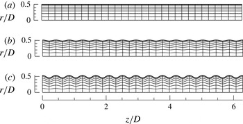
Figure 2. Spectral element meshes, each with 240 elements in the meridional semi-plane. Here,
 $h$
is the peak-to-peak wave height and
$h$
is the peak-to-peak wave height and
 $a=h/2$
is the corrugation amplitude. The labels match those used in table 1: (a) smooth-wall pipe; (b)
$a=h/2$
is the corrugation amplitude. The labels match those used in table 1: (a) smooth-wall pipe; (b)
 $h_{314}^{+}=20$
; (c)
$h_{314}^{+}=20$
; (c)
 $h_{314}^{+}=50$
.
$h_{314}^{+}=50$
.
We note that since the corrugated domains are two-dimensional, it follows that the associated time-mean flows and local turbulent statistics are too. When we present one-dimensional profile data for turbulence statistics below, the values have also been averaged in the streamwise direction. This implies that profiles representing averages of product terms, such as Reynolds stresses, contain contributions from streamwise averages of products of the deviations of the time-mean flow velocity components from the streamwise-mean profile as well as from the streamwise averages of the local fluctuation products. Contributions from the time-mean or ‘coherent’ streamwise fluctuations from the mean velocity profile are typically only significant within one corrugation height of the mean radius.
3.2. Validation for smooth-pipe flow
Due to the lack of availability of wavy-wall pipe flow data, the veracity of the smooth-wall turbulent-flow calculations was tested by comparing statistical profiles with laser Doppler velocimetry (LDV) measurements obtained at
 $\mathit{Re}_{{\it\tau}}=314.5$
by den Toonder & Nieuwstadt (Reference den Toonder and Nieuwstadt1997). Comparisons were presented in figure 7 of Blackburn et al. (Reference Blackburn, Ooi and Chong2007). It should be noted that statistical data were only calculated after all the initial transients had convected out of the computational domain and the flow field had reached a statistically stationary state. The mean velocity showed excellent agreement with the measurements. The comparison of the second-order statistics between the DNS and measurements was also very good, except in the near-wall region where measurement inaccuracies became apparent. The r.m.s. profile of the radial fluctuations was also slightly but consistently lower than the experimental measurements. Such deviations are, however, common, e.g. as observed by Westerweel (Reference Westerweel1993) and den Toonder & Nieuwstadt (Reference den Toonder and Nieuwstadt1997). The reasons behind this underestimation of the radial velocity r.m.s. apparently remains an open question.
$\mathit{Re}_{{\it\tau}}=314.5$
by den Toonder & Nieuwstadt (Reference den Toonder and Nieuwstadt1997). Comparisons were presented in figure 7 of Blackburn et al. (Reference Blackburn, Ooi and Chong2007). It should be noted that statistical data were only calculated after all the initial transients had convected out of the computational domain and the flow field had reached a statistically stationary state. The mean velocity showed excellent agreement with the measurements. The comparison of the second-order statistics between the DNS and measurements was also very good, except in the near-wall region where measurement inaccuracies became apparent. The r.m.s. profile of the radial fluctuations was also slightly but consistently lower than the experimental measurements. Such deviations are, however, common, e.g. as observed by Westerweel (Reference Westerweel1993) and den Toonder & Nieuwstadt (Reference den Toonder and Nieuwstadt1997). The reasons behind this underestimation of the radial velocity r.m.s. apparently remains an open question.
4. Axisymmetric laminar flows
Steady laminar axisymmetric flows were computed on a domain of one axial wavelength,
 $L_{m}=2{\rm\pi}D/15$
, and steady flows were computed using an adaptation of a time-stepping code that uses a matrix-free Newton–Raphson method based on Stokes preconditioning (Tuckerman & Barkley Reference Tuckerman, Barkley, Doedel and Tuckerman2000; Blackburn Reference Blackburn2002). Results were computed for
$L_{m}=2{\rm\pi}D/15$
, and steady flows were computed using an adaptation of a time-stepping code that uses a matrix-free Newton–Raphson method based on Stokes preconditioning (Tuckerman & Barkley Reference Tuckerman, Barkley, Doedel and Tuckerman2000; Blackburn Reference Blackburn2002). Results were computed for
 $\mathit{Re}_{{\it\tau}}=27.8$
, 39.3, 55.6 and 78.6 (
$\mathit{Re}_{{\it\tau}}=27.8$
, 39.3, 55.6 and 78.6 (
 $\mathit{Re}_{D}\approx 300{-}3000$
). These laminar flows for all wave heights investigated are stable to axisymmetric disturbances at these Reynolds numbers. A further check that the axisymmetric flows are stable to axisymmetric perturbations in the wavy pipe can be made by computing the flow in the whole domain using the two-dimensional unsteady Navier–Stokes equations, and perturbing the solution impulsively with white noise. This was done at
$\mathit{Re}_{D}\approx 300{-}3000$
). These laminar flows for all wave heights investigated are stable to axisymmetric disturbances at these Reynolds numbers. A further check that the axisymmetric flows are stable to axisymmetric perturbations in the wavy pipe can be made by computing the flow in the whole domain using the two-dimensional unsteady Navier–Stokes equations, and perturbing the solution impulsively with white noise. This was done at
 $\mathit{Re}_{{\it\tau}}=78.6$
for the largest wave height (case G), and it was found that the perturbed solution returned to the steady-state solution. We note that these flows may be unstable to non-axisymmetric disturbances. Stability analysis carried out by Loh & Blackburn (Reference Loh and Blackburn2011) for corrugated pipes with a similar corrugation wavelength to that employed here showed that the flow first became unstable to disturbances with azimuthal wavenumbers
$\mathit{Re}_{{\it\tau}}=78.6$
for the largest wave height (case G), and it was found that the perturbed solution returned to the steady-state solution. We note that these flows may be unstable to non-axisymmetric disturbances. Stability analysis carried out by Loh & Blackburn (Reference Loh and Blackburn2011) for corrugated pipes with a similar corrugation wavelength to that employed here showed that the flow first became unstable to disturbances with azimuthal wavenumbers
 $k_{o}=3$
, 4 and at bulk Reynolds numbers similar to the upper end of the range we have used.
$k_{o}=3$
, 4 and at bulk Reynolds numbers similar to the upper end of the range we have used.
Example streamwise velocity profiles extracted at the axial location corresponding to
 $R_{min}$
for laminar flows computed at
$R_{min}$
for laminar flows computed at
 $\mathit{Re}_{{\it\tau}}=55.6$
are shown in figure 3(a). (It should be noted that the pipe cross-section of minimum radius is located at
$\mathit{Re}_{{\it\tau}}=55.6$
are shown in figure 3(a). (It should be noted that the pipe cross-section of minimum radius is located at
 $z=L_{m}/2$
.) The profile for the smooth pipe matches the parabolic Hagen–Poiseuille solution, and has a peak velocity of twice the bulk velocity. The rough-wall profiles are distorted near the wall but approach a parabolic profile near the pipe centreline. The velocity defect plot, shown in figure 3(b), confirms that well away from the wall, the profiles all approach a common shape. Thus, the axial-average flow near the centre of the pipe is not greatly influenced by the detail of the wall corrugation, other than through the influence this has on the surface shear stress.
$z=L_{m}/2$
.) The profile for the smooth pipe matches the parabolic Hagen–Poiseuille solution, and has a peak velocity of twice the bulk velocity. The rough-wall profiles are distorted near the wall but approach a parabolic profile near the pipe centreline. The velocity defect plot, shown in figure 3(b), confirms that well away from the wall, the profiles all approach a common shape. Thus, the axial-average flow near the centre of the pipe is not greatly influenced by the detail of the wall corrugation, other than through the influence this has on the surface shear stress.
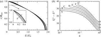
Figure 3. Velocity profiles for laminar flow at
 $\mathit{Re}_{{\it\tau}}=55.6$
. (a) Profiles obtained at the axial location of the minimum pipe radius,
$\mathit{Re}_{{\it\tau}}=55.6$
. (a) Profiles obtained at the axial location of the minimum pipe radius,
 $R_{min}=\bar{R}-a$
, normalized by the bulk velocity in that section. The arrow indicates increasing wave height,
$R_{min}=\bar{R}-a$
, normalized by the bulk velocity in that section. The arrow indicates increasing wave height,
 $h$
. (b) Axial-average velocity defect. Note the vertical separation applied to the curves.
$h$
. (b) Axial-average velocity defect. Note the vertical separation applied to the curves.
We now turn to an examination of the friction factor,
 ${\it\lambda}$
, for the laminar flows. From velocity profiles extracted at
${\it\lambda}$
, for the laminar flows. From velocity profiles extracted at
 $z=L_{m}/2$
, the volumetric flow rates were computed, followed by the bulk-flow Reynolds numbers based on the mean diameter, i.e.
$z=L_{m}/2$
, the volumetric flow rates were computed, followed by the bulk-flow Reynolds numbers based on the mean diameter, i.e.
 $\mathit{Re}_{D}$
, and then from (2.3) the pipe friction factor,
$\mathit{Re}_{D}$
, and then from (2.3) the pipe friction factor,
 ${\it\lambda}$
. The data for the four laminar-flow Reynolds numbers are shown in figure 4. Several points are worth noting. First, on this log–log plot, lines of constant
${\it\lambda}$
. The data for the four laminar-flow Reynolds numbers are shown in figure 4. Several points are worth noting. First, on this log–log plot, lines of constant
 $\mathit{Re}_{{\it\tau}}$
have a slope of
$\mathit{Re}_{{\it\tau}}$
have a slope of
 $-2$
(see (2.3)), hence each set of data falls along such a line. Second, the data for the smooth pipe fall exactly on the analytical result
$-2$
(see (2.3)), hence each set of data falls along such a line. Second, the data for the smooth pipe fall exactly on the analytical result
 ${\it\lambda}=64/\mathit{Re}_{D}$
, as expected (the slope and intercept values for a power-law curve fit through the four smooth-pipe data points match the analytical values to five-digit accuracy). Third, the friction factors for the wavy-wall cases are greater than those for a smooth pipe. While it is conventional to accept that in laminar flow roughness has no effect on the friction factor, some reflection suggests that this is an approximate result for small roughness height that can only be true in the smooth-pipe limit. Fourth, power laws fitted through the wavy wall results (the dashed and solid lines in figure 4) have slopes that progressively become somewhat less negative with increasing wave height.
${\it\lambda}=64/\mathit{Re}_{D}$
, as expected (the slope and intercept values for a power-law curve fit through the four smooth-pipe data points match the analytical values to five-digit accuracy). Third, the friction factors for the wavy-wall cases are greater than those for a smooth pipe. While it is conventional to accept that in laminar flow roughness has no effect on the friction factor, some reflection suggests that this is an approximate result for small roughness height that can only be true in the smooth-pipe limit. Fourth, power laws fitted through the wavy wall results (the dashed and solid lines in figure 4) have slopes that progressively become somewhat less negative with increasing wave height.
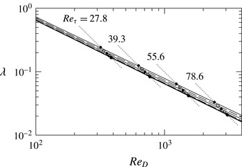
Figure 4. Pipe friction factor
 ${\it\lambda}$
as a function of
${\it\lambda}$
as a function of
 $\mathit{Re}_{D}$
for laminar flows at four different values of
$\mathit{Re}_{D}$
for laminar flows at four different values of
 $\mathit{Re}_{{\it\tau}}$
. In each set, the lowest point corresponds to the smooth pipe and the upper point corresponds to the highest-amplitude wave, case G. The solid and dashed lines through the data points show best-fit power laws,
$\mathit{Re}_{{\it\tau}}$
. In each set, the lowest point corresponds to the smooth pipe and the upper point corresponds to the highest-amplitude wave, case G. The solid and dashed lines through the data points show best-fit power laws,
 ${\it\lambda}=64/[1-0.8(h/D)^{1.2}]\mathit{Re}_{D}$
.
${\it\lambda}=64/[1-0.8(h/D)^{1.2}]\mathit{Re}_{D}$
.
5. Inner and outer normalizations in the turbulent regime
5.1. Mean velocity profiles
The effects of the corrugation height and Reynolds number are evident in the behaviour of the mean velocity profile. Figure 5 presents mean velocity profiles in both inner and velocity defect forms. The results for the smooth-wall pipe (case A) are also included for comparison. The mean statistics in the corrugated pipe were computed by averaging over
 $z{-}{\it\theta}$
planes uniformly up to the minimum sensible radius
$z{-}{\it\theta}$
planes uniformly up to the minimum sensible radius
 $R_{min}$
. The velocity field around the wavy surface is strongly influenced by the surface profile. This is clearly seen by comparing the near-wall flow with the smooth-wall case. With an increase in corrugation height, the maximum centreline velocity decreases in comparison to the smooth pipe. The offset in the maximum mean velocity profiles depends on the magnitude of the corrugation amplitude, as suggested by Blackburn et al. (Reference Blackburn, Ooi and Chong2007). By plotting the mean velocity profiles for case G for
$R_{min}$
. The velocity field around the wavy surface is strongly influenced by the surface profile. This is clearly seen by comparing the near-wall flow with the smooth-wall case. With an increase in corrugation height, the maximum centreline velocity decreases in comparison to the smooth pipe. The offset in the maximum mean velocity profiles depends on the magnitude of the corrugation amplitude, as suggested by Blackburn et al. (Reference Blackburn, Ooi and Chong2007). By plotting the mean velocity profiles for case G for
 $\mathit{Re}_{{\it\tau}}=180\,250$
and 314, figure 5(a) shows an increasing downward shift of the inner-normalized profiles with increasing Reynolds number. The near-wall velocity profiles also remain substantially different from the smooth-wall pipe flow. The existence of the no-slip boundary condition causes the mean velocity profiles to vary sharply within the near-wall corrugated region. Hence, the overall velocity field (averaged over
$\mathit{Re}_{{\it\tau}}=180\,250$
and 314, figure 5(a) shows an increasing downward shift of the inner-normalized profiles with increasing Reynolds number. The near-wall velocity profiles also remain substantially different from the smooth-wall pipe flow. The existence of the no-slip boundary condition causes the mean velocity profiles to vary sharply within the near-wall corrugated region. Hence, the overall velocity field (averaged over
 $z{-}{\it\theta}$
planes) exhibits a larger momentum deficit when compared with the smooth-wall flow. In contrast, the mean velocity profiles in defect form (figure 5
b) exhibit agreement for all cases in the region
$z{-}{\it\theta}$
planes) exhibits a larger momentum deficit when compared with the smooth-wall flow. In contrast, the mean velocity profiles in defect form (figure 5
b) exhibit agreement for all cases in the region
 ${\it\eta}\geqslant 0.2$
for the present conditions. This is in accord with Townsend’s wall-similarity hypothesis (Townsend Reference Townsend1956). Observations similar to these were made by Shockling et al. (Reference Shockling, Allen and Smits2006) for distributed roughness pipe flows in the transitionally and fully rough regimes. The mean profiles systematically vary as a function of corrugation amplitude within the corrugated sublayer. This is consistent with the study of Wu & Christensen (Reference Wu and Christensen2007).
${\it\eta}\geqslant 0.2$
for the present conditions. This is in accord with Townsend’s wall-similarity hypothesis (Townsend Reference Townsend1956). Observations similar to these were made by Shockling et al. (Reference Shockling, Allen and Smits2006) for distributed roughness pipe flows in the transitionally and fully rough regimes. The mean profiles systematically vary as a function of corrugation amplitude within the corrugated sublayer. This is consistent with the study of Wu & Christensen (Reference Wu and Christensen2007).
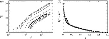
Figure 5. Mean velocity profile for different corrugation heights at
 $\mathit{Re}_{{\it\tau}}=314$
and for different values of
$\mathit{Re}_{{\it\tau}}=314$
and for different values of
 $\mathit{Re}_{{\it\tau}}$
at the highest corrugation height (
$\mathit{Re}_{{\it\tau}}$
at the highest corrugation height (
 $h/D=0.46024$
): (a) inner scaling and (b) outer scaling (velocity defect law). The symbol shapes for the DNS data are given in table 1.
$h/D=0.46024$
): (a) inner scaling and (b) outer scaling (velocity defect law). The symbol shapes for the DNS data are given in table 1.
The effect of the corrugation height is characterized here using a corrugation amplitude,
 $a=h/2$
. This has similarity to an equivalent sand-grain roughness height,
$a=h/2$
. This has similarity to an equivalent sand-grain roughness height,
 $k_{s}$
(Nikuradse Reference Nikuradse1933; Schlichting Reference Schlichting1936). When
$k_{s}$
(Nikuradse Reference Nikuradse1933; Schlichting Reference Schlichting1936). When
 $a$
increases to become comparable to
$a$
increases to become comparable to
 ${\it\nu}/u_{{\it\tau}}$
, the inner-scaled profiles exhibit a downward shift relative to the smooth-wall profile. The wall-normal extent of this deficit, which can be interpreted as an internal layer within which the length scales imposed by the corrugated surface directly impact the dynamics, is surface-dependent, with the highest corrugation height showing the largest wall-normal extent of velocity deficit (
${\it\nu}/u_{{\it\tau}}$
, the inner-scaled profiles exhibit a downward shift relative to the smooth-wall profile. The wall-normal extent of this deficit, which can be interpreted as an internal layer within which the length scales imposed by the corrugated surface directly impact the dynamics, is surface-dependent, with the highest corrugation height showing the largest wall-normal extent of velocity deficit (
 $y^{+}\geqslant 50$
). Consistent with enhanced drag, this deficit increases with increasing corrugation height, and is largest for case G. For the set of conditions explored, the mean velocity profile can be expressed as
$y^{+}\geqslant 50$
). Consistent with enhanced drag, this deficit increases with increasing corrugation height, and is largest for case G. For the set of conditions explored, the mean velocity profile can be expressed as
 $$\begin{eqnarray}U^{+}=\frac{1}{{\it\kappa}}\ln y^{+}+A_{o}-{\rm\Delta}U^{+},\end{eqnarray}$$
where
 ${\rm\Delta}U^{+}$
is denoted as the corrugation function. Analogous to the roughness function of Hama (Reference Hama1954), the corrugation function depends on
${\rm\Delta}U^{+}$
is denoted as the corrugation function. Analogous to the roughness function of Hama (Reference Hama1954), the corrugation function depends on
 $a^{+}$
or
$a^{+}$
or
 $h^{+}$
. The relationship between
$h^{+}$
. The relationship between
 ${\rm\Delta}U^{+}$
and
${\rm\Delta}U^{+}$
and
 $a^{+}$
follows from the concept of equivalent sand-grain roughness. For the profiles of figure 6(a),
$a^{+}$
follows from the concept of equivalent sand-grain roughness. For the profiles of figure 6(a),
 ${\rm\Delta}U^{+}=4.45$
and 8.0 for
${\rm\Delta}U^{+}=4.45$
and 8.0 for
 $h_{314}^{+}=20$
and 50 respectively. According to the analogy with equivalent sand-grain roughness, for sufficiently large
$h_{314}^{+}=20$
and 50 respectively. According to the analogy with equivalent sand-grain roughness, for sufficiently large
 $a^{+}$
there should be a loss of dependence on viscosity, allowing the log-law velocity profile to be written as
$a^{+}$
there should be a loss of dependence on viscosity, allowing the log-law velocity profile to be written as
 $$\begin{eqnarray}U^{+}=\frac{1}{{\it\kappa}}\ln \left(\frac{y}{a}\right)+A^{\prime },\end{eqnarray}$$
where
 $A^{\prime }$
is the effective corrugation function, analogous to the Nikuradse roughness function.
$A^{\prime }$
is the effective corrugation function, analogous to the Nikuradse roughness function.
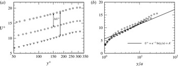
Figure 6. Mean velocity profile plotted (a) against
 $y^{+}$
showing the logarithmic region and (b) against
$y^{+}$
showing the logarithmic region and (b) against
 $y/a$
. The data sets are as for figure 5.
$y/a$
. The data sets are as for figure 5.
Figure 6(b) plots
 $U^{+}$
versus
$U^{+}$
versus
 $y/a$
. In the fully rough regime, the viscous sublayer no longer exists. Consistently, the effective corrugation function appears to approach an approximately constant value of
$y/a$
. In the fully rough regime, the viscous sublayer no longer exists. Consistently, the effective corrugation function appears to approach an approximately constant value of
 $A^{\prime }\simeq 5.6$
, which is smaller than the Nikuradse roughness function value of approximately 8.5 in the fully rough regime. We also observe that for the conditions explored herein the increasing
$A^{\prime }\simeq 5.6$
, which is smaller than the Nikuradse roughness function value of approximately 8.5 in the fully rough regime. We also observe that for the conditions explored herein the increasing
 $a^{+}$
profiles at fixed
$a^{+}$
profiles at fixed
 $\mathit{Re}_{{\it\tau}}$
continue to exhibit a small but apparently persistent variation. This probably indicates that the largest
$\mathit{Re}_{{\it\tau}}$
continue to exhibit a small but apparently persistent variation. This probably indicates that the largest
 $a^{+}$
condition may still not be in the fully rough (fully corrugated) regime. For completeness we note that from (5.1) and (5.2), the corrugation function in the fully rough regime is given by
$a^{+}$
condition may still not be in the fully rough (fully corrugated) regime. For completeness we note that from (5.1) and (5.2), the corrugation function in the fully rough regime is given by
 $$\begin{eqnarray}{\rm\Delta}U^{+}=\frac{1}{{\it\kappa}}\ln a^{+}+A_{o}-A^{\prime }.\end{eqnarray}$$
In the present work, the corrugation function
 ${\rm\Delta}U^{+}$
is plotted against the ES as shown in figure 7. For comparison, data from Napoli et al. (Reference Napoli, Armenio and De Marchis2008), Schultz & Flack (Reference Schultz and Flack2009) and De Marchis & Napoli (Reference De Marchis and Napoli2012) are included in the plot. The results are presented for
${\rm\Delta}U^{+}$
is plotted against the ES as shown in figure 7. For comparison, data from Napoli et al. (Reference Napoli, Armenio and De Marchis2008), Schultz & Flack (Reference Schultz and Flack2009) and De Marchis & Napoli (Reference De Marchis and Napoli2012) are included in the plot. The results are presented for
 $0\leqslant \mathit{ES}\leqslant 0.38$
at the highest Reynolds number and are found to show a trend similar to other observations. Napoli et al. (Reference Napoli, Armenio and De Marchis2008) observed linear variation of
$0\leqslant \mathit{ES}\leqslant 0.38$
at the highest Reynolds number and are found to show a trend similar to other observations. Napoli et al. (Reference Napoli, Armenio and De Marchis2008) observed linear variation of
 ${\rm\Delta}U^{+}$
for
${\rm\Delta}U^{+}$
for
 $\mathit{ES}\leqslant 0.15$
, whereas the corrugation function for sinusoidally corrugated pipes increases linearly up to approximately
$\mathit{ES}\leqslant 0.15$
, whereas the corrugation function for sinusoidally corrugated pipes increases linearly up to approximately
 $\mathit{ES}\sim 0.24$
.
$\mathit{ES}\sim 0.24$
.
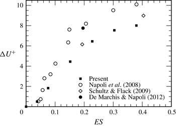
Figure 7. Dependence of the roughness function
 ${\rm\Delta}U^{+}$
on the ES of the wall corrugations at
${\rm\Delta}U^{+}$
on the ES of the wall corrugations at
 $\mathit{Re}_{{\it\tau}}=314$
. Data for different types of wall corrugation and
$\mathit{Re}_{{\it\tau}}=314$
. Data for different types of wall corrugation and
 $\mathit{Re}_{{\it\tau}}$
from Napoli et al. (Reference Napoli, Armenio and De Marchis2008), Schultz & Flack (Reference Schultz and Flack2009) and De Marchis & Napoli (Reference De Marchis and Napoli2012) are included here for comparison.
$\mathit{Re}_{{\it\tau}}$
from Napoli et al. (Reference Napoli, Armenio and De Marchis2008), Schultz & Flack (Reference Schultz and Flack2009) and De Marchis & Napoli (Reference De Marchis and Napoli2012) are included here for comparison.
5.2. Velocity fluctuation r.m.s. profiles
The effects of roughness in the inner and outer regions of the flow are examined in the context of Townsend’s outer similarity hypothesis by comparing the turbulence intensity profiles from the wavy- and smooth-wall pipes. Figure 8(a–f) shows the turbulence intensities in the streamwise, wall-normal and azimuthal directions as normalized by the friction velocity, and for both inner- and outer-normalized corrugation heights. The root-mean-square (r.m.s.) profiles of the streamwise velocity fluctuations in figure 8(a) do not vary with the presence of corrugation for
 $y^{+}\geqslant 60$
, and agree very well with the results for the smooth-pipe flow in the outer region of the flow. As the wall is approached, however, the wavy-wall data fall below the smooth-wall data. This is generically consistent with the findings for other rough-wall pipe flows, e.g. Allen et al. (Reference Allen, Shockling, Kunkel and Smits2007).
$y^{+}\geqslant 60$
, and agree very well with the results for the smooth-pipe flow in the outer region of the flow. As the wall is approached, however, the wavy-wall data fall below the smooth-wall data. This is generically consistent with the findings for other rough-wall pipe flows, e.g. Allen et al. (Reference Allen, Shockling, Kunkel and Smits2007).
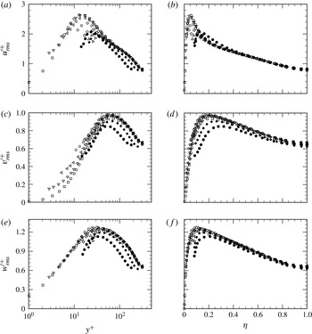
Figure 8. Root mean square profiles of turbulent intensities for different corrugation heights at
 $\mathit{Re}_{{\it\tau}}=314$
and for different values of
$\mathit{Re}_{{\it\tau}}=314$
and for different values of
 $\mathit{Re}_{{\it\tau}}$
at the largest corrugation height (
$\mathit{Re}_{{\it\tau}}$
at the largest corrugation height (
 $h/D=0.46024$
): (a,b) streamwise velocity fluctuation; (c,d) radial velocity fluctuation; (e,f) azimuthal velocity fluctuation; (a,c,e) profiles representing inner normalization; (b,d,f) profiles in outer-scaled variables. The data sets are as for figure 5.
$h/D=0.46024$
): (a,b) streamwise velocity fluctuation; (c,d) radial velocity fluctuation; (e,f) azimuthal velocity fluctuation; (a,c,e) profiles representing inner normalization; (b,d,f) profiles in outer-scaled variables. The data sets are as for figure 5.
The profiles of radial and tangential velocity fluctuation (see figure 8
c–f) also merge outside the corrugated sublayer. These findings are consistent with the notion of outer-layer similarity. Relative to
 ${u^{\prime }}_{rms}^{+}$
, the effect of the roughness is more subtly realized for the
${u^{\prime }}_{rms}^{+}$
, the effect of the roughness is more subtly realized for the
 ${v^{\prime }}_{rms}^{+}$
and
${v^{\prime }}_{rms}^{+}$
and
 ${w^{\prime }}_{rms}^{+}$
profiles, whose near-wall peak values and locations show little change from the smooth-wall profile. Overall, the main influence on the
${w^{\prime }}_{rms}^{+}$
profiles, whose near-wall peak values and locations show little change from the smooth-wall profile. Overall, the main influence on the
 ${u^{\prime }}_{rms}^{+}$
profile is that its peak value attenuates near the wavy wall and shifts away from the wall with increasing
${u^{\prime }}_{rms}^{+}$
profile is that its peak value attenuates near the wavy wall and shifts away from the wall with increasing
 $h^{+}$
. On the other hand, the primary apparent effect on the
$h^{+}$
. On the other hand, the primary apparent effect on the
 ${v^{\prime }}_{rms}^{+}$
and
${v^{\prime }}_{rms}^{+}$
and
 ${w^{\prime }}_{rms}^{+}$
profiles is that the locations of their peaks shift slightly towards the pipe centre with increasing
${w^{\prime }}_{rms}^{+}$
profiles is that the locations of their peaks shift slightly towards the pipe centre with increasing
 $h^{+}$
.
$h^{+}$
.
By considering increasing
 $\mathit{Re}_{{\it\tau}}$
for a fixed corrugation height, the traditional description leads to the expectation of encountering a dynamically smooth wall, followed by a transitionally rough wall and culminating with a fully rough-wall flow. The Reynolds number range of the present study (
$\mathit{Re}_{{\it\tau}}$
for a fixed corrugation height, the traditional description leads to the expectation of encountering a dynamically smooth wall, followed by a transitionally rough wall and culminating with a fully rough-wall flow. The Reynolds number range of the present study (
 $\mathit{Re}_{{\it\tau}}=180,250,314$
), however, apparently only resides in the transitional rough-wall regime. This is even so for the case of the largest corrugation height (
$\mathit{Re}_{{\it\tau}}=180,250,314$
), however, apparently only resides in the transitional rough-wall regime. This is even so for the case of the largest corrugation height (
 $h/D=0.07952$
), which corresponds to
$h/D=0.07952$
), which corresponds to
 $h^{+}\approx 30,40$
and 50 respectively. Figure 8 also displays the inner- and outer-normalized turbulence intensities for the cases G180 and G250. These data indicate an increasing trend in the peak values of
$h^{+}\approx 30,40$
and 50 respectively. Figure 8 also displays the inner- and outer-normalized turbulence intensities for the cases G180 and G250. These data indicate an increasing trend in the peak values of
 ${v^{\prime }}_{rms}^{+}$
and
${v^{\prime }}_{rms}^{+}$
and
 ${w^{\prime }}_{rms}^{+}$
with
${w^{\prime }}_{rms}^{+}$
with
 $\mathit{Re}_{{\it\tau}}$
, while the peak in the
$\mathit{Re}_{{\it\tau}}$
, while the peak in the
 ${u^{\prime }}_{rms}^{+}$
profile decreases. Continued profile variations of the type displayed for increasing
${u^{\prime }}_{rms}^{+}$
profile decreases. Continued profile variations of the type displayed for increasing
 $h^{+}$
provide evidence of transitional rough-wall flow. The data in the outer region are in imperfect agreement with Townsend’s similarity hypothesis, indicating results similar to those presented by Flack et al. (Reference Flack, Schultz and Shapiro2005). Likely reasons for this include low Reynolds number and insufficiently small
$h^{+}$
provide evidence of transitional rough-wall flow. The data in the outer region are in imperfect agreement with Townsend’s similarity hypothesis, indicating results similar to those presented by Flack et al. (Reference Flack, Schultz and Shapiro2005). Likely reasons for this include low Reynolds number and insufficiently small
 ${\it\delta}/h$
.
${\it\delta}/h$
.
5.3. Reynolds shear-stress profile
Profiles of the Reynolds shear stress are presented in figure 9. Over a considerable outer-region extent, and for inner- and outer-normalized distance from the wall, the wavy-wall profiles
 $T_{u}^{+}=-\langle uv\rangle ^{+}$
convincingly merge with the smooth-wall profile. The effect of corrugation becomes stronger only at high corrugation height, and thus the profiles near the wavy-wall fall below the smooth-wall data. Under outer normalization the corrugated- and smooth-wall profiles consistently merge at a wall-normal position just beyond the peak of
$T_{u}^{+}=-\langle uv\rangle ^{+}$
convincingly merge with the smooth-wall profile. The effect of corrugation becomes stronger only at high corrugation height, and thus the profiles near the wavy-wall fall below the smooth-wall data. Under outer normalization the corrugated- and smooth-wall profiles consistently merge at a wall-normal position just beyond the peak of
 $T_{u}^{+}$
. As discussed in § 7, this behaviour correlates with an important feature of the mean dynamical balance. The influence of
$T_{u}^{+}$
. As discussed in § 7, this behaviour correlates with an important feature of the mean dynamical balance. The influence of
 $\mathit{Re}_{{\it\tau}}$
is also apparent. The inner-normalized profiles of figure 9(a) exhibit an expected shift with increasing
$\mathit{Re}_{{\it\tau}}$
is also apparent. The inner-normalized profiles of figure 9(a) exhibit an expected shift with increasing
 $\mathit{Re}_{{\it\tau}}$
. The outer-normalized profiles of figure 9(b), however, show excellent agreement beyond the
$\mathit{Re}_{{\it\tau}}$
. The outer-normalized profiles of figure 9(b), however, show excellent agreement beyond the
 $T_{u}^{+}$
peak, suggesting robust support for outer similarity in the domain where the mean dynamics is inertially dominated (see § 7).
$T_{u}^{+}$
peak, suggesting robust support for outer similarity in the domain where the mean dynamics is inertially dominated (see § 7).
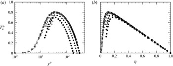
Figure 9. Reynolds shear-stress profiles for different corrugation heights at
 $\mathit{Re}_{{\it\tau}}=314$
and for different values of
$\mathit{Re}_{{\it\tau}}=314$
and for different values of
 $\mathit{Re}_{{\it\tau}}$
at the largest corrugation height (
$\mathit{Re}_{{\it\tau}}$
at the largest corrugation height (
 $h/D=0.46024$
): (a) inner scaling and (b) outer scaling. The data sets are as for figure 5.
$h/D=0.46024$
): (a) inner scaling and (b) outer scaling. The data sets are as for figure 5.
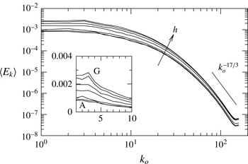
Figure 10. Average kinetic energy in non-axisymmetric modes as a function of the azimuthal wavenumber
 $k_{o}$
for turbulent flow at
$k_{o}$
for turbulent flow at
 $\mathit{Re}_{{\it\tau}}=314$
. Values are normalized by the average axisymmetric energy,
$\mathit{Re}_{{\it\tau}}=314$
. Values are normalized by the average axisymmetric energy,
 $\langle E_{0}\rangle$
. Inset: data replotted in linear coordinates, emphasizing the emergence with increasing corrugation height of a peak in energy at low wavenumbers centred around
$\langle E_{0}\rangle$
. Inset: data replotted in linear coordinates, emphasizing the emergence with increasing corrugation height of a peak in energy at low wavenumbers centred around
 $k_{o}=3$
.
$k_{o}=3$
.
6. Other features of wavy-wall turbulence
Three additional features of wavy-wall turbulence are now noted and described. Figure 10 shows the normalized azimuthal wavenumber spectra of the time-averaged kinetic energy in the modes with
 $k_{0}>0$
for turbulent flow at
$k_{0}>0$
for turbulent flow at
 $\mathit{Re}_{{\it\tau}}=314$
. The measure of kinetic energy is defined as
$\mathit{Re}_{{\it\tau}}=314$
. The measure of kinetic energy is defined as
 $$\begin{eqnarray}E_{k_{o}}=\frac{1}{2AU^{2}}\int _{A}\hat{\boldsymbol{u}}_{k_{o}}^{+}\boldsymbol{\cdot }\hat{\boldsymbol{u}}_{k_{o}}^{\ast +}\,r\,\text{d}A,\end{eqnarray}$$
where
 $U$
is the local mean velocity,
$U$
is the local mean velocity,
 $\hat{\boldsymbol{u}}_{k_{o}}^{+\ast }$
represents the complex conjugate of velocity data in the
$\hat{\boldsymbol{u}}_{k_{o}}^{+\ast }$
represents the complex conjugate of velocity data in the
 $k_{o}$
th azimuthal Fourier mode and
$k_{o}$
th azimuthal Fourier mode and
 $A=L\bar{R}={\rm\pi}D^{2}$
is the area of the meridional semi-plane. It can be seen that there is more than a four-decade spread of energy over the represented non-axisymmetric wavenumbers, and that aliasing has a detectable but small effect at the highest wavenumbers. The inset to figure 10 demonstrates that with increasing corrugation amplitude, a peak in the azimuthal energy spectrum begins to emerge at
$A=L\bar{R}={\rm\pi}D^{2}$
is the area of the meridional semi-plane. It can be seen that there is more than a four-decade spread of energy over the represented non-axisymmetric wavenumbers, and that aliasing has a detectable but small effect at the highest wavenumbers. The inset to figure 10 demonstrates that with increasing corrugation amplitude, a peak in the azimuthal energy spectrum begins to emerge at
 $k_{o}=3$
. Loh & Blackburn (Reference Loh and Blackburn2011) found that for a corrugation wavelength of
$k_{o}=3$
. Loh & Blackburn (Reference Loh and Blackburn2011) found that for a corrugation wavelength of
 $L_{m}/D=0.5$
, similar to the presently employed value of
$L_{m}/D=0.5$
, similar to the presently employed value of
 $L_{m}/D\approx 0.419$
, steady axisymmetric flow in corrugated pipes became unstable to global modes with comparatively low azimuthal wavenumbers of
$L_{m}/D\approx 0.419$
, steady axisymmetric flow in corrugated pipes became unstable to global modes with comparatively low azimuthal wavenumbers of
 $k_{o}=3$
and
$k_{o}=3$
and
 $k_{o}=4$
. Hence, the emergence of this peak with increasing corrugation height at
$k_{o}=4$
. Hence, the emergence of this peak with increasing corrugation height at
 $k_{o}=3$
seems likely to be related to this instability mechanism.
$k_{o}=3$
seems likely to be related to this instability mechanism.
The total viscous and pressure drag exerted on the wall were computed, thus allowing their contribution to the total to be assessed as a function of ES. Figure 11 shows the pressure drag relative to the total drag as a function of the corrugation height for the four laminar-flow and one turbulent-flow Reynolds numbers studied here. It is observed that the relative proportion of pressure drag increases with the Reynolds number, as with the corrugation height. It is notable that when
 $\mathit{Re}_{{\it\tau}}\geqslant 55.6$
, the pressure drag component can be up to 50 % or more for
$\mathit{Re}_{{\it\tau}}\geqslant 55.6$
, the pressure drag component can be up to 50 % or more for
 $\mathit{ES}\gtrsim 0.3$
(
$\mathit{ES}\gtrsim 0.3$
(
 $h/\bar{R}\gtrsim 0.1$
, see table 1). As shown in figure 11 at
$h/\bar{R}\gtrsim 0.1$
, see table 1). As shown in figure 11 at
 $\mathit{Re}_{{\it\tau}}=314$
, the increasing relative importance of the pressure component of the overall average wall drag more than counteracts the decrease in the viscous component. At the maximum corrugation height (case G), the overall contribution of pressure drag is relatively higher, and accounts for approximately 85 % of the total. This suggests that the flow is approaching the fully rough-wall flow condition, since asymptotically all the drag derives from the pressure difference in this case. This correlates with the findings discussed relative to the effective corrugation function of figure 6.
$\mathit{Re}_{{\it\tau}}=314$
, the increasing relative importance of the pressure component of the overall average wall drag more than counteracts the decrease in the viscous component. At the maximum corrugation height (case G), the overall contribution of pressure drag is relatively higher, and accounts for approximately 85 % of the total. This suggests that the flow is approaching the fully rough-wall flow condition, since asymptotically all the drag derives from the pressure difference in this case. This correlates with the findings discussed relative to the effective corrugation function of figure 6.
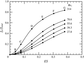
Figure 11. Pressure drag as a proportion of total drag for laminar and turbulent flows, plotted as a function of the ES of the wall waviness.
Although a regular corrugated wall (with no geometric randomness) is only a simplified representation of the generic ‘rough’ wall, an attempt was made to estimate the equivalent sand roughness. Nikuradse’s classic experimental data helps us to carry out the primary comparison. Nikuradse (Reference Nikuradse1933) obtained these data by glueing various fine-sized sands inside smooth pipes. The friction factors
 ${\it\lambda}$
versus
${\it\lambda}$
versus
 $\mathit{Re}_{D}$
are plotted for the geometries B–G as shown in figure 12 at
$\mathit{Re}_{D}$
are plotted for the geometries B–G as shown in figure 12 at
 $\mathit{Re}_{{\it\tau}}=314$
. Only the values of the friction factor for case E (open squares) are shown in the laminar regime in order to avoid clutter. The small open circles represent Nikuradse’s data for different relative roughnesses
$\mathit{Re}_{{\it\tau}}=314$
. Only the values of the friction factor for case E (open squares) are shown in the laminar regime in order to avoid clutter. The small open circles represent Nikuradse’s data for different relative roughnesses
 $\bar{R}/k$
. The onset of transition from laminar to turbulent flow takes place for the bulk-flow Reynolds number
$\bar{R}/k$
. The onset of transition from laminar to turbulent flow takes place for the bulk-flow Reynolds number
 $\mathit{Re}_{D}\sim 2500$
in both data sets; thus the transitional value of
$\mathit{Re}_{D}\sim 2500$
in both data sets; thus the transitional value of
 ${\it\lambda}$
for case E falls within the scatter band of Nikuradse’s data, and this is also similar to the linear instability values found by Loh & Blackburn (Reference Loh and Blackburn2011). It is interesting to observe that the onset of turbulence begins more rapidly with increasing
${\it\lambda}$
for case E falls within the scatter band of Nikuradse’s data, and this is also similar to the linear instability values found by Loh & Blackburn (Reference Loh and Blackburn2011). It is interesting to observe that the onset of turbulence begins more rapidly with increasing
 $\mathit{Re}_{D}$
for the corrugated wall cases than for sand roughness. We note that the turbulent-flow data sets represented in figure 12 were generated by restarting at successively lower Reynolds number from the previous simulation beginning with
$\mathit{Re}_{D}$
for the corrugated wall cases than for sand roughness. We note that the turbulent-flow data sets represented in figure 12 were generated by restarting at successively lower Reynolds number from the previous simulation beginning with
 $\mathit{Re}_{{\it\tau}}=314$
. The apparent sudden transition from turbulent to laminar states observed in figure 12 for
$\mathit{Re}_{{\it\tau}}=314$
. The apparent sudden transition from turbulent to laminar states observed in figure 12 for
 $\mathit{Re}_{D}\approx 2000$
may correspond to subcritical transition behaviour – a point not examined in the linear stability analysis of Loh & Blackburn (Reference Loh and Blackburn2011). Finally, it seems likely that the smooth transition behaviour observed by Nikuradse (Reference Nikuradse1933) for all roughness heights is related to the use of randomly distributed roughness in his study.
$\mathit{Re}_{D}\approx 2000$
may correspond to subcritical transition behaviour – a point not examined in the linear stability analysis of Loh & Blackburn (Reference Loh and Blackburn2011). Finally, it seems likely that the smooth transition behaviour observed by Nikuradse (Reference Nikuradse1933) for all roughness heights is related to the use of randomly distributed roughness in his study.
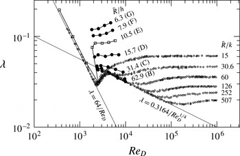
Figure 12. Nikuradse’s data (Nikuradse Reference Nikuradse1933) for the pipe friction factor as functions of
 $\mathit{Re}_{D}$
and the relative roughness
$\mathit{Re}_{D}$
and the relative roughness
 $\bar{R}/k$
(open circles). Also shown is the variation of the friction factor with
$\bar{R}/k$
(open circles). Also shown is the variation of the friction factor with
 $\mathit{Re}_{D}$
for the corrugated wall at various values of
$\mathit{Re}_{D}$
for the corrugated wall at various values of
 $\mathit{Re}_{D}$
, computed for cases B–G (filled circles except case E) and case E (open squares), together with the relative corrugation height
$\mathit{Re}_{D}$
, computed for cases B–G (filled circles except case E) and case E (open squares), together with the relative corrugation height
 $\bar{R}/h$
.
$\bar{R}/h$
.
The values of
 ${\it\lambda}$
for the present turbulent-flow simulations can be compared with Nikuradse’s data for similar values of
${\it\lambda}$
for the present turbulent-flow simulations can be compared with Nikuradse’s data for similar values of
 $\bar{R}/h$
and
$\bar{R}/h$
and
 $\bar{R}/k$
, although it is difficult to draw any firm conclusions. If one accepts the criteria set in § 5.1 for the analogy of corrugation height to equivalent sand roughness, then one should see the data for
$\bar{R}/k$
, although it is difficult to draw any firm conclusions. If one accepts the criteria set in § 5.1 for the analogy of corrugation height to equivalent sand roughness, then one should see the data for
 $\bar{R}/h=62.9$
or
$\bar{R}/h=62.9$
or
 $\bar{R}/a=31.45$
(case B) asymptote close to Nikuradse’s data for
$\bar{R}/a=31.45$
(case B) asymptote close to Nikuradse’s data for
 $\bar{R}/k_{s}=30.6$
. Similarly, the data for
$\bar{R}/k_{s}=30.6$
. Similarly, the data for
 $R/h=31.4$
or
$R/h=31.4$
or
 $\bar{R}/a=15.7$
asymptotically approach Nikuradse’s data for
$\bar{R}/a=15.7$
asymptotically approach Nikuradse’s data for
 $\bar{R}/k=15$
. At a minimum, these findings suggest that further investigations are warranted.
$\bar{R}/k=15$
. At a minimum, these findings suggest that further investigations are warranted.
7. Scaling mean dynamics
Beyond the transitional regime, the leading-order balances of terms in the mean momentum equation for smooth-wall flows organize into a four-layer structure (Wei et al.
Reference Wei, Fife, Klewicki and McMurtry2005a
,Reference Wei, McMurtry, Klewicki and Fife
b
; Klewicki et al.
Reference Klewicki, Chin, Blackburn, Ooi and Marusic2012). The Reynolds number scaling behaviour associated with the layer properties (see table 2 for layer widths and velocity increments) has been analytically determined and empirically verified (Fife, Klewicki & Wei Reference Fife, Klewicki and Wei2009; Klewicki Reference Klewicki2013b
). It is relevant that two of the four layer widths vary with the Reynolds number in proportion to the intermediate length,
 $({\it\nu}{\it\delta}/u_{{\it\tau}})^{1/2}$
, where
$({\it\nu}{\it\delta}/u_{{\it\tau}})^{1/2}$
, where
 ${\it\delta}$
is either the pipe radius, half channel height or boundary layer thickness. The significance of these findings to rough-wall flows is associated with an intermediate length being the geometric mean of the inner and outer length scales (i.e.
${\it\delta}$
is either the pipe radius, half channel height or boundary layer thickness. The significance of these findings to rough-wall flows is associated with an intermediate length being the geometric mean of the inner and outer length scales (i.e.
 $({\it\nu}{\it\delta}/u_{{\it\tau}})^{1/2}=({\it\delta}\times ({\it\nu}/u_{{\it\tau}}))^{1/2}$
), and thus inherently depending upon the overall separation of scales, which increases with
$({\it\nu}{\it\delta}/u_{{\it\tau}})^{1/2}=({\it\delta}\times ({\it\nu}/u_{{\it\tau}}))^{1/2}$
), and thus inherently depending upon the overall separation of scales, which increases with
 $\mathit{Re}_{{\it\tau}}$
. Clarity regarding the dynamical implications of this is gained by briefly reviewing the nature of the leading-order balances of terms across the flow.
$\mathit{Re}_{{\it\tau}}$
. Clarity regarding the dynamical implications of this is gained by briefly reviewing the nature of the leading-order balances of terms across the flow.
Table 2. Scaling characteristics of the layer width and velocity increments of smooth-wall pipe flow associated with the mean momentum equation.

7.1. The four-layer structure
A sketch representing the smooth-wall four-layer structure at a fixed Reynolds number is illustrated in figure 13. Not all of the terms in (2.17) are of leading order throughout, and this leads to a different magnitude ordering of terms in each of the four layers: layer I,
 $|\mathit{PG}|\cong |\mathit{VF}|\gg |\mathit{TI}|$
; layer II,
$|\mathit{PG}|\cong |\mathit{VF}|\gg |\mathit{TI}|$
; layer II,
 $|\mathit{VF}|\cong |\mathit{TI}|\gg |\mathit{PG}|$
; layer III,
$|\mathit{VF}|\cong |\mathit{TI}|\gg |\mathit{PG}|$
; layer III,
 $|\mathit{VF}|\cong |\mathit{TI}|\cong |\mathit{PG}|$
; layer IV,
$|\mathit{VF}|\cong |\mathit{TI}|\cong |\mathit{PG}|$
; layer IV,
 $|\mathit{TI}|\cong |\mathit{PG}|\gg |\mathit{VF}|$
. For smooth-wall pipe flow, the magnitude of the ratio (
$|\mathit{TI}|\cong |\mathit{PG}|\gg |\mathit{VF}|$
. For smooth-wall pipe flow, the magnitude of the ratio (
 $\mathit{VF}/\mathit{TI}$
) exceeds unity in layer I, indicating a nominal balance between the pressure gradient and the mean viscous force. Thus, layer I coincides with the viscous sublayer, which is obliterated in the presence of dynamically significant roughness. In layer II, the dominant balance is between the viscous stress gradient and the Reynolds stress gradient. Conventional notions lead to the expectation that for transitionally or fully rough flows, layer II is obliterated as well, since roughness is typically viewed as generating inertially dominated flow from the roughness crests outward. Consistent with the results of Mehdi et al. (Reference Mehdi, Klewicki and White2013), the results presented below reveal that this is distinctly not the case. Namely, layer II continues to exist. Across layer III, all three terms are of equal order, but by layer IV the
$\mathit{VF}/\mathit{TI}$
) exceeds unity in layer I, indicating a nominal balance between the pressure gradient and the mean viscous force. Thus, layer I coincides with the viscous sublayer, which is obliterated in the presence of dynamically significant roughness. In layer II, the dominant balance is between the viscous stress gradient and the Reynolds stress gradient. Conventional notions lead to the expectation that for transitionally or fully rough flows, layer II is obliterated as well, since roughness is typically viewed as generating inertially dominated flow from the roughness crests outward. Consistent with the results of Mehdi et al. (Reference Mehdi, Klewicki and White2013), the results presented below reveal that this is distinctly not the case. Namely, layer II continues to exist. Across layer III, all three terms are of equal order, but by layer IV the
 $\mathit{VF}$
term loses leading-order importance and there exists a dominant balance between the
$\mathit{VF}$
term loses leading-order importance and there exists a dominant balance between the
 $\mathit{PG}$
and
$\mathit{PG}$
and
 $\mathit{TI}$
terms.
$\mathit{TI}$
terms.
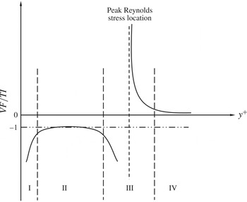
Figure 13. Sketch of the four layers of turbulent flow in a smooth-wall pipe at fixed Reynolds number (Wei et al.
Reference Wei, Fife, Klewicki and McMurtry2005a
). It should be noted that across layer III the
 $\mathit{TI}$
term changes sign and there is an exchange of dominant balance. From the outer edge of layer III to the pipe centreline the leading-order mean dynamics is governed by the inertial terms,
$\mathit{TI}$
term changes sign and there is an exchange of dominant balance. From the outer edge of layer III to the pipe centreline the leading-order mean dynamics is governed by the inertial terms,
 $\mathit{TI}$
and
$\mathit{TI}$
and
 $\mathit{PG}$
.
$\mathit{PG}$
.
Roughness imposes scales of motion in the range between
 $O({\it\nu}/u_{{\it\tau}})$
and
$O({\it\nu}/u_{{\it\tau}})$
and
 $O({\it\delta})$
. These scales modify the distribution of dynamically relevant length scales with distance from the wall. The net result of this is that the layer structure that describes the leading-order mean dynamics, and, in particular, the position at which the
$O({\it\delta})$
. These scales modify the distribution of dynamically relevant length scales with distance from the wall. The net result of this is that the layer structure that describes the leading-order mean dynamics, and, in particular, the position at which the
 $\mathit{VF}$
term loses leading order, now becomes a function of the roughness and Reynolds number. Apart from this, the analysis and evidence presented by Mehdi et al. (Reference Mehdi, Klewicki and White2013) indicate that the overall scale separation in rough-wall flows can be segregated into contributions associated with the scale separation between the inner and roughness scale and the roughness and outer scale. By adopting a natural extension of the smooth-wall theory, they further show that a unifying element in describing the structure of both smooth- and rough-wall flows is that the onset of inertially dominated mean dynamics is described by an intermediate length scale. For the smooth-wall flow, this length scale is analytically shown to be solely a function of the overall scale separation (as reflected in the value of
$\mathit{VF}$
term loses leading order, now becomes a function of the roughness and Reynolds number. Apart from this, the analysis and evidence presented by Mehdi et al. (Reference Mehdi, Klewicki and White2013) indicate that the overall scale separation in rough-wall flows can be segregated into contributions associated with the scale separation between the inner and roughness scale and the roughness and outer scale. By adopting a natural extension of the smooth-wall theory, they further show that a unifying element in describing the structure of both smooth- and rough-wall flows is that the onset of inertially dominated mean dynamics is described by an intermediate length scale. For the smooth-wall flow, this length scale is analytically shown to be solely a function of the overall scale separation (as reflected in the value of
 $\mathit{Re}_{{\it\tau}}$
), while in the rough-wall case, this intermediate scale is a function of the relative scale separations between the inner, roughness and outer scales, and the Reynolds number (overall scale separation).
$\mathit{Re}_{{\it\tau}}$
), while in the rough-wall case, this intermediate scale is a function of the relative scale separations between the inner, roughness and outer scales, and the Reynolds number (overall scale separation).
Due to the geometric complexity of the roughnesses employed in the experiments of Mehdi et al. (Reference Mehdi, Klewicki and White2013), the wall-normal location of the peak in
 $T_{u}$
was used as a surrogate for the intermediate length scale, i.e. a surrogate for the position from the wall to the outer edge of layer III – the position where the leading-order mean dynamics becomes wholly inertial. A remarkable feature of the present wavy-wall roughness is that it allows one to consider normalizations of (2.17) in which the driving mean pressure gradient is given by an explicit analytical expression that includes the effect of corrugation height. Thus, for example, the definition of
$T_{u}$
was used as a surrogate for the intermediate length scale, i.e. a surrogate for the position from the wall to the outer edge of layer III – the position where the leading-order mean dynamics becomes wholly inertial. A remarkable feature of the present wavy-wall roughness is that it allows one to consider normalizations of (2.17) in which the driving mean pressure gradient is given by an explicit analytical expression that includes the effect of corrugation height. Thus, for example, the definition of
 ${\it\varepsilon}$
in (2.19) allows one to recover the exact inner-normalized mean momentum equation for smooth-wall pipe flow, i.e. as
${\it\varepsilon}$
in (2.19) allows one to recover the exact inner-normalized mean momentum equation for smooth-wall pipe flow, i.e. as
 $h^{+}\rightarrow 0$
. More importantly, this representation also allows the description of mean dynamics given by Mehdi et al. (Reference Mehdi, Klewicki and White2013) to be formally tested by replacing the surrogate intermediate length with an exact analytical expression.
$h^{+}\rightarrow 0$
. More importantly, this representation also allows the description of mean dynamics given by Mehdi et al. (Reference Mehdi, Klewicki and White2013) to be formally tested by replacing the surrogate intermediate length with an exact analytical expression.
The ratio of the gradient of the viscous stress to the gradient of the Reynolds stress is plotted against the wall-normal distance
 $y^{+}$
in figure 14(a). As generically observed by Mehdi et al. (Reference Mehdi, Klewicki and White2013), the ratio (
$y^{+}$
in figure 14(a). As generically observed by Mehdi et al. (Reference Mehdi, Klewicki and White2013), the ratio (
 $\mathit{VF}/\mathit{TI}$
) attains a value of approximately
$\mathit{VF}/\mathit{TI}$
) attains a value of approximately
 $-1$
interior to where the
$-1$
interior to where the
 $\mathit{TI}$
term crosses zero (i.e. where the ratio asymptotes to
$\mathit{TI}$
term crosses zero (i.e. where the ratio asymptotes to
 $\pm \infty$
). In this region of the flow, there is also more data spread than farther from the wall. The profile variability here is a direct effect of the roughness, while the scatter within each profile is a consequence of taking the ratio of derivative quantities in a region where the statistical convergence below the roughness elements is not as good as away from the wall. For all corrugation heights and Reynolds numbers explored, the data of figure 14 unambiguously reveal the existence of layer II. The physical significance of this is that the
$\pm \infty$
). In this region of the flow, there is also more data spread than farther from the wall. The profile variability here is a direct effect of the roughness, while the scatter within each profile is a consequence of taking the ratio of derivative quantities in a region where the statistical convergence below the roughness elements is not as good as away from the wall. For all corrugation heights and Reynolds numbers explored, the data of figure 14 unambiguously reveal the existence of layer II. The physical significance of this is that the
 $\mathit{VF}$
term retains leading order. The highest corrugation height (case G) exhibits a noticeable
$\mathit{VF}$
term retains leading order. The highest corrugation height (case G) exhibits a noticeable
 $y^{+}$
shift in the position of layer II as the Reynolds number increases from 180 to 314. Moreover, the combined effect of the Reynolds number and corrugation height does not noticeably influence the existence of the other two distinct layers (layers III and IV), albeit their
$y^{+}$
shift in the position of layer II as the Reynolds number increases from 180 to 314. Moreover, the combined effect of the Reynolds number and corrugation height does not noticeably influence the existence of the other two distinct layers (layers III and IV), albeit their
 $y^{+}$
position is clearly influenced by
$y^{+}$
position is clearly influenced by
 $\mathit{Re}_{{\it\tau}}$
and
$\mathit{Re}_{{\it\tau}}$
and
 $h^{+}$
. As anticipated, for all values of
$h^{+}$
. As anticipated, for all values of
 $h^{+}$
greater than 5, layer I is completely destroyed.
$h^{+}$
greater than 5, layer I is completely destroyed.

Figure 14. Ratio of the mean viscous force to the mean effect of turbulent inertia: (a) versus
 $y^{+}$
; (b) versus
$y^{+}$
; (b) versus
 ${\hat{y}}$
, the intermediate normalization that yields the invariant form (7.6). Inset: the data replotted showing the shift in layer II with increasing Reynolds number. The data sets are the same as in figure 5.
${\hat{y}}$
, the intermediate normalization that yields the invariant form (7.6). Inset: the data replotted showing the shift in layer II with increasing Reynolds number. The data sets are the same as in figure 5.
7.2. Scaling via invariant representation of the mean dynamics
We now determine an invariant form of the relevant mean momentum equation that is applicable over most of the flow domain and that inherently accounts for the combined effects of roughness and Reynolds number. We begin by noting that the inner and outer variables
 $y^{+}$
and
$y^{+}$
and
 ${\it\eta}$
are appropriate to the inner and outer domains respectively. Layer III in figure 13 is of particular interest, since it has been shown (for smooth-wall flow) that its structure is replicated as a function of
${\it\eta}$
are appropriate to the inner and outer domains respectively. Layer III in figure 13 is of particular interest, since it has been shown (for smooth-wall flow) that its structure is replicated as a function of
 $y$
over a hierarchy of scaling layers that span from
$y$
over a hierarchy of scaling layers that span from
 $O({\it\nu}/u_{{\it\tau}})$
to
$O({\it\nu}/u_{{\it\tau}})$
to
 $O({\it\delta})$
(Fife et al.
Reference Fife, Klewicki and Wei2009). The distinctive feature of each layer in this hierarchy, and layer III, is that all of the terms in (2.17) have the same order of magnitude.
$O({\it\delta})$
(Fife et al.
Reference Fife, Klewicki and Wei2009). The distinctive feature of each layer in this hierarchy, and layer III, is that all of the terms in (2.17) have the same order of magnitude.
According to the approach used for channel flow, rescaling is most easily accomplished for the differentials
 $\text{d}y^{+}$
and
$\text{d}y^{+}$
and
 $\text{d}T_{u}^{+}$
(Wei et al.
Reference Wei, Fife, Klewicki and McMurtry2005a
). The simplest successful rescaling takes the form
$\text{d}T_{u}^{+}$
(Wei et al.
Reference Wei, Fife, Klewicki and McMurtry2005a
). The simplest successful rescaling takes the form
 $$\begin{eqnarray}\text{d}y^{+}={\rm\pi}_{1}\,\text{d}{\hat{y}},\quad \text{d}T_{u}^{+}={\rm\pi}_{2}\,\text{d}\hat{T}_{u},\quad \text{d}U^{+}=\text{d}\hat{U} ,\end{eqnarray}$$
where
 $\hat{U}$
and
$\hat{U}$
and
 $\hat{T}_{u}$
are the rescaled
$\hat{T}_{u}$
are the rescaled
 $O(1)$
functions of
$O(1)$
functions of
 ${\hat{y}}$
and
${\hat{y}}$
and
 ${\it\varepsilon}$
, and
${\it\varepsilon}$
, and
 ${\rm\pi}_{1}$
and
${\rm\pi}_{1}$
and
 ${\rm\pi}_{2}$
are scaling parameters, functions of
${\rm\pi}_{2}$
are scaling parameters, functions of
 ${\it\varepsilon}$
, to be determined. The terms in (2.17) then transform as
${\it\varepsilon}$
, to be determined. The terms in (2.17) then transform as
 $$\begin{eqnarray}\frac{\text{d}^{2}U^{+}}{\text{d}y^{+2}}=\frac{1}{{\rm\pi}_{1}^{2}}\frac{\text{d}^{2}\hat{U} }{\text{d}{\hat{y}}^{2}},\quad \frac{\text{d}T_{u}^{+}}{\text{d}y^{+}}=\frac{{\rm\pi}_{2}}{{\rm\pi}_{1}}\frac{\text{d}\hat{T}_{u}}{\text{d}{\hat{y}}}.\end{eqnarray}$$
Invariance is satisfied when the derivatives on the right of (7.2), namely
 $\text{d}^{2}\hat{U} /\text{d}{\hat{y}}^{2}$
and
$\text{d}^{2}\hat{U} /\text{d}{\hat{y}}^{2}$
and
 $\text{d}\hat{T}_{u}/\text{d}{\hat{y}}$
, are rescaled to formally become
$\text{d}\hat{T}_{u}/\text{d}{\hat{y}}$
, are rescaled to formally become
 $O(1)$
quantities for all Reynolds numbers and roughness heights. By the requirement established above, the orders of magnitude of both terms on the right, namely
$O(1)$
quantities for all Reynolds numbers and roughness heights. By the requirement established above, the orders of magnitude of both terms on the right, namely
 $1/{\rm\pi}_{1}^{2}$
and
$1/{\rm\pi}_{1}^{2}$
and
 ${\rm\pi}_{2}/{\rm\pi}_{1}$
, must match (in order of magnitude) the third term in (2.17), namely
${\rm\pi}_{2}/{\rm\pi}_{1}$
, must match (in order of magnitude) the third term in (2.17), namely
 ${\it\varepsilon}^{2}:{\rm\pi}_{1}^{-2}={\rm\pi}_{2}/{\rm\pi}_{1}={\it\varepsilon}^{2}$
. This is only possible if
${\it\varepsilon}^{2}:{\rm\pi}_{1}^{-2}={\rm\pi}_{2}/{\rm\pi}_{1}={\it\varepsilon}^{2}$
. This is only possible if
 ${\rm\pi}_{2}={\it\varepsilon},{\rm\pi}_{1}={\it\varepsilon}^{-1}$
.
${\rm\pi}_{2}={\it\varepsilon},{\rm\pi}_{1}={\it\varepsilon}^{-1}$
.
Thus, from (7.1)
 $$\begin{eqnarray}\text{d}y^{+}={\it\varepsilon}^{-1}\,\text{d}{\hat{y}},\quad \text{d}T_{u}^{+}={\it\varepsilon}\,\text{d}\hat{T}_{u}.\end{eqnarray}$$
Integrating (7.3) gives two integration constants which are chosen to be
 $y_{m}^{+}$
and
$y_{m}^{+}$
and
 $T_{um}^{+}$
; they are the values of
$T_{um}^{+}$
; they are the values of
 $y^{+}$
and
$y^{+}$
and
 $T_{u}^{+}$
where
$T_{u}^{+}$
where
 ${\hat{y}}=0$
and
${\hat{y}}=0$
and
 $\hat{T}_{u}=0$
. The result is
$\hat{T}_{u}=0$
. The result is
 $$\begin{eqnarray}y^{+}=y_{m}^{+}+{\it\varepsilon}^{-1}{\hat{y}},\quad T_{u}^{+}=T_{um}^{+}+{\it\varepsilon}\hat{T}_{u},\end{eqnarray}$$
where the quantities with subscript
 $m$
are the values of those variables at the maximum point
$m$
are the values of those variables at the maximum point
 $y_{m}^{+}$
of
$y_{m}^{+}$
of
 $T_{u}^{+}$
. The rescaled intermediate variables now become
$T_{u}^{+}$
. The rescaled intermediate variables now become
 $$\begin{eqnarray}{\hat{y}}={\it\varepsilon}(y^{+}-y_{m}^{+}),\quad \hat{T}_{u}={\it\varepsilon}^{-1}(T_{u}^{+}-T_{um}^{+}),\quad \hat{U} =U^{+}-U_{m}^{+},\end{eqnarray}$$
where
 $y_{m}^{+}$
and
$y_{m}^{+}$
and
 $T_{um}^{+}$
are the maximum Reynolds shear-stress location and value respectively and
$T_{um}^{+}$
are the maximum Reynolds shear-stress location and value respectively and
 $U_{m}^{+}$
is the value of the mean streamwise velocity at the maximum point
$U_{m}^{+}$
is the value of the mean streamwise velocity at the maximum point
 $y_{m}^{+}$
.
$y_{m}^{+}$
.
Normalization of the mean momentum equation according to these variables results in
 $$\begin{eqnarray}\frac{\text{d}^{2}\hat{U} }{\text{d}{\hat{y}}^{2}}+\frac{\text{d}\hat{T}_{u}}{\text{d}{\hat{y}}}+1=0\end{eqnarray}$$
and thus provides the desired parameter-free representation in which all scaled terms are formally represented as being
 $O(1)$
. The rescaled functions satisfy
$O(1)$
. The rescaled functions satisfy
 $\hat{T}_{u}(0)=\text{d}\hat{T}_{u}/\text{d}{\hat{y}}(0)=0$
,
$\hat{T}_{u}(0)=\text{d}\hat{T}_{u}/\text{d}{\hat{y}}(0)=0$
,
 $\text{d}^{2}\hat{U} /\text{d}{\hat{y}}^{2}(0)=-1$
. It should be noted that the present rescaling differs from that used for smooth-wall flows. In the smooth-wall case, the intermediate variable is equal to the geometric mean between the inner and outer length scales, i.e.
$\text{d}^{2}\hat{U} /\text{d}{\hat{y}}^{2}(0)=-1$
. It should be noted that the present rescaling differs from that used for smooth-wall flows. In the smooth-wall case, the intermediate variable is equal to the geometric mean between the inner and outer length scales, i.e.
 ${\hat{y}}=y/({\it\delta}({\it\nu}/u_{{\it\tau}}))^{1/2}$
. Due to (2.19), the new meso-variable takes the form
${\hat{y}}=y/({\it\delta}({\it\nu}/u_{{\it\tau}}))^{1/2}$
. Due to (2.19), the new meso-variable takes the form
 ${\hat{y}}=y((V_{o}/V)/({\it\delta}{\it\nu}/u_{{\it\tau}}))^{1/2}$
, where the factor
${\hat{y}}=y((V_{o}/V)/({\it\delta}{\it\nu}/u_{{\it\tau}}))^{1/2}$
, where the factor
 $V_{o}/V=1+h^{2}/(8\bar{R}^{2})$
analytically accounts for the influence of varying corrugation height. While the present analyses support and illuminate the notions associated with the dynamical relevance of the intermediate length scale in rough-wall flows, we stress that this analysis still requires knowledge of the location of the
$V_{o}/V=1+h^{2}/(8\bar{R}^{2})$
analytically accounts for the influence of varying corrugation height. While the present analyses support and illuminate the notions associated with the dynamical relevance of the intermediate length scale in rough-wall flows, we stress that this analysis still requires knowledge of the location of the
 $T_{u}^{+}$
peak, which cannot be obtained without first carrying out the simulations. Hence, we still do not have an a priori description of the effect of a particular roughness.
$T_{u}^{+}$
peak, which cannot be obtained without first carrying out the simulations. Hence, we still do not have an a priori description of the effect of a particular roughness.
The ratio of
 $\mathit{VF}/\mathit{TI}$
profiles is plotted versus
$\mathit{VF}/\mathit{TI}$
profiles is plotted versus
 ${\hat{y}}$
in figure 14(b). As is apparent, from layer III outward, the agreement between the different
${\hat{y}}$
in figure 14(b). As is apparent, from layer III outward, the agreement between the different
 $h^{+}$
and
$h^{+}$
and
 $\mathit{Re}_{{\it\tau}}$
profiles is much improved. Furthermore, a good portion of the scatter in layer II is rationally attributable to the aforementioned uncertainty associated with statistical convergence, while the remaining profile variations in this region are probably associated with genuine dependences on
$\mathit{Re}_{{\it\tau}}$
profiles is much improved. Furthermore, a good portion of the scatter in layer II is rationally attributable to the aforementioned uncertainty associated with statistical convergence, while the remaining profile variations in this region are probably associated with genuine dependences on
 $h^{+}$
and
$h^{+}$
and
 $\mathit{Re}_{{\it\tau}}$
. These findings are consistent with the smooth-wall analysis, indicating that, with increasing
$\mathit{Re}_{{\it\tau}}$
. These findings are consistent with the smooth-wall analysis, indicating that, with increasing
 $\mathit{Re}_{{\it\tau}}$
, self-similar mean dynamics is most rapidly developed in a domain beginning near the outer edge of layer III (i.e. the log layer), while over a region interior to that point, and extending to the lower portion of layer II, Reynolds number invariance is established more slowly (Klewicki Reference Klewicki2013b
). These findings are also in accord with the rough-wall observations of Mehdi et al. (Reference Mehdi, Klewicki and White2013), indicating that interior to the outer edge of layer III the interactions involving the viscous and inertial forces are, in general, significantly influenced by the scales of motion imposed by the roughness. Conversely, beyond layer III they surmise that for roughnesses that sufficiently three-dimensionalize and/or reduce the characteristic scales of the layer II vorticity field the flow properties beyond layer III (i.e. in the domain where the leading-order dynamics is wholly inertial) become independent of the roughness details, and thus satisfy Townsend’s outer similarity hypotheses. The results of §§ 5.2 and 5.3 generally support these findings in that outer similarity is empirically observed to hold near to, or slightly beyond, the wall-normal location of the peak in
$\mathit{Re}_{{\it\tau}}$
, self-similar mean dynamics is most rapidly developed in a domain beginning near the outer edge of layer III (i.e. the log layer), while over a region interior to that point, and extending to the lower portion of layer II, Reynolds number invariance is established more slowly (Klewicki Reference Klewicki2013b
). These findings are also in accord with the rough-wall observations of Mehdi et al. (Reference Mehdi, Klewicki and White2013), indicating that interior to the outer edge of layer III the interactions involving the viscous and inertial forces are, in general, significantly influenced by the scales of motion imposed by the roughness. Conversely, beyond layer III they surmise that for roughnesses that sufficiently three-dimensionalize and/or reduce the characteristic scales of the layer II vorticity field the flow properties beyond layer III (i.e. in the domain where the leading-order dynamics is wholly inertial) become independent of the roughness details, and thus satisfy Townsend’s outer similarity hypotheses. The results of §§ 5.2 and 5.3 generally support these findings in that outer similarity is empirically observed to hold near to, or slightly beyond, the wall-normal location of the peak in
 $T_{u}^{+}$
.
$T_{u}^{+}$
.
The veracity of the scaling depicted in figure 14(b) is more directly tested by examining whether the solutions of (7.6) are indeed invariant for variations in
 $h^{+}$
and
$h^{+}$
and
 $\mathit{Re}_{{\it\tau}}$
. The mean velocity and Reynolds shear-stress profiles ranging from smooth to the maximum
$\mathit{Re}_{{\it\tau}}$
. The mean velocity and Reynolds shear-stress profiles ranging from smooth to the maximum
 $h^{+}$
explored are plotted in figure 15(a,b). The result is encouraging, as these profiles exhibit convincing invariance, except possibly for the
$h^{+}$
explored are plotted in figure 15(a,b). The result is encouraging, as these profiles exhibit convincing invariance, except possibly for the
 $h^{+}=50$
case, where the roughness height is approximately
$h^{+}=50$
case, where the roughness height is approximately
 $1/6$
of the mean pipe radius. This is likely to be a case where the vorticity field in layer II does not sufficiently three-dimensionalize at small scales, and outer similarity breaks down. Here, it is also relevant to note that the invariance approximated in figure 15 should improve with increasing
$1/6$
of the mean pipe radius. This is likely to be a case where the vorticity field in layer II does not sufficiently three-dimensionalize at small scales, and outer similarity breaks down. Here, it is also relevant to note that the invariance approximated in figure 15 should improve with increasing
 $\mathit{Re}_{{\it\tau}}$
.
$\mathit{Re}_{{\it\tau}}$
.
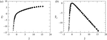
Figure 15. Meso-normalized profiles of the mean velocity (a) and Reynolds shear stress (b) for turbulent flow in smooth and wavy-walled pipes. The data sets are the same as in figure 5.
Evidence in support of this interpretation is given by figure 16, which shows the normalized magnitude of the mean vorticity,
 ${\it\Omega}_{z}=-\text{d}U/\text{d}y$
. Analysis of the mean momentum equation reveals that the mean vorticity will decay from its wall value of
${\it\Omega}_{z}=-\text{d}U/\text{d}y$
. Analysis of the mean momentum equation reveals that the mean vorticity will decay from its wall value of
 $|{\it\Omega}_{z}^{+}|=1$
to a value that is
$|{\it\Omega}_{z}^{+}|=1$
to a value that is
 $O({\it\varepsilon})$
by
$O({\it\varepsilon})$
by
 $y^{+}=O({\it\varepsilon}^{-1})$
, and then decay from there to
$y^{+}=O({\it\varepsilon}^{-1})$
, and then decay from there to
 $O({\it\varepsilon}^{2})$
by
$O({\it\varepsilon}^{2})$
by
 $y^{+}=O({\it\varepsilon}^{-2})$
, e.g. Klewicki (Reference Klewicki2013b
). These features predicted by the analysis can be directly tested by plotting the data according to the normalization of figure 16. Smooth-wall pipe data in the range
$y^{+}=O({\it\varepsilon}^{-2})$
, e.g. Klewicki (Reference Klewicki2013b
). These features predicted by the analysis can be directly tested by plotting the data according to the normalization of figure 16. Smooth-wall pipe data in the range
 $1800\leqslant \mathit{Re}_{{\it\tau}}\leqslant 530\,000$
(not shown in figure 16) and boundary layer data in the range
$1800\leqslant \mathit{Re}_{{\it\tau}}\leqslant 530\,000$
(not shown in figure 16) and boundary layer data in the range
 $1000\leqslant \mathit{Re}_{{\it\tau}}\leqslant 17\,000$
confirm that, for all
$1000\leqslant \mathit{Re}_{{\it\tau}}\leqslant 17\,000$
confirm that, for all
 $\mathit{Re}_{{\it\tau}}$
,
$\mathit{Re}_{{\it\tau}}$
,
 ${\it\varepsilon}^{-1}|{\it\Omega}_{z}^{+}|=1$
at the outer edge of layer III, i.e.
${\it\varepsilon}^{-1}|{\it\Omega}_{z}^{+}|=1$
at the outer edge of layer III, i.e.
 ${\it\varepsilon}y^{+}\simeq 2.6$
(Klewicki Reference Klewicki2013b
). Furthermore, by using the position of the peak in
${\it\varepsilon}y^{+}\simeq 2.6$
(Klewicki Reference Klewicki2013b
). Furthermore, by using the position of the peak in
 $T_{u}^{+}$
as a surrogate for the intermediate length scale, Mehdi et al. (Reference Mehdi, Klewicki and White2013) showed that, except for large organized roughness (i.e. large two-dimensional transverse bars), this same condition is also satisfied for a range of roughnesses covering over a decade in
$T_{u}^{+}$
as a surrogate for the intermediate length scale, Mehdi et al. (Reference Mehdi, Klewicki and White2013) showed that, except for large organized roughness (i.e. large two-dimensional transverse bars), this same condition is also satisfied for a range of roughnesses covering over a decade in
 $\mathit{Re}_{{\it\tau}}$
and over two decades in
$\mathit{Re}_{{\it\tau}}$
and over two decades in
 $k_{s}^{+}$
. Physically, this observed decay rate stems from the reduction in scale and three-dimensionalization of the near-wall vorticity field, caused by vorticity stretching, and that results in an exchange of mean enstrophy to fluctuating enstrophy (Klewicki Reference Klewicki2013a
). In accord with this interpretation, the
$k_{s}^{+}$
. Physically, this observed decay rate stems from the reduction in scale and three-dimensionalization of the near-wall vorticity field, caused by vorticity stretching, and that results in an exchange of mean enstrophy to fluctuating enstrophy (Klewicki Reference Klewicki2013a
). In accord with this interpretation, the
 $h^{+}=50$
profile in figure 16 does not quite adhere to the predicted decay rate, presumably due to the roughness-induced motions in layer II being too large and organized. Again, the distinct (and remarkable) advantage of the present analysis is that its explicit representation of the pressure drop as a function of the corrugation height allows the present scaling theory to be analytically tested.
$h^{+}=50$
profile in figure 16 does not quite adhere to the predicted decay rate, presumably due to the roughness-induced motions in layer II being too large and organized. Again, the distinct (and remarkable) advantage of the present analysis is that its explicit representation of the pressure drop as a function of the corrugation height allows the present scaling theory to be analytically tested.
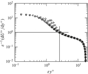
Figure 16. Meso-normalized mean velocity gradient (
 $-{\it\Omega}_{z}$
) profiles for smooth and wavy-walled pipes. The horizontal line denotes
$-{\it\Omega}_{z}$
) profiles for smooth and wavy-walled pipes. The horizontal line denotes
 ${\it\varepsilon}^{-1}|{\it\Omega}_{z}^{+}|=1$
and the vertical line denotes
${\it\varepsilon}^{-1}|{\it\Omega}_{z}^{+}|=1$
and the vertical line denotes
 ${\it\varepsilon}y^{+}=2.6$
. The expression for
${\it\varepsilon}y^{+}=2.6$
. The expression for
 ${\it\varepsilon}$
is given by (2.19).
${\it\varepsilon}$
is given by (2.19).
8. Discussion and conclusions
Direct numerical simulation data were presented for both laminar and turbulent flows through wavy-walled pipes of fixed axial wavelength and with a number of corrugation amplitudes. The largest Reynolds number considered was
 $\mathit{Re}_{{\it\tau}}=314$
, corresponding in the smooth-pipe case to
$\mathit{Re}_{{\it\tau}}=314$
, corresponding in the smooth-pipe case to
 $\mathit{Re}_{D}\approx 9930$
. The radial height of the largest corrugation corresponded to approximately 0.16 times the mean radius of the wavy-wall pipe. Within these limits, it is believed that the turbulent-flow data represent and support scaling predictions derived from analysis of the mean momentum equation.
$\mathit{Re}_{D}\approx 9930$
. The radial height of the largest corrugation corresponded to approximately 0.16 times the mean radius of the wavy-wall pipe. Within these limits, it is believed that the turbulent-flow data represent and support scaling predictions derived from analysis of the mean momentum equation.
The data from laminar flows exhibit flow separation and increased pressure drag with increasing surface waviness. One of the notable findings is that the pressure drag accounts for more than 50 % of the total for
 $\mathit{Re}_{{\it\tau}}\geqslant 55.6$
and
$\mathit{Re}_{{\it\tau}}\geqslant 55.6$
and
 $\mathit{ES}\geqslant 0.26$
, even in the absence of (mean) flow separation. Moreover, the laminar flow inside a wavy-wall pipe follows a linear friction-factor relationship with the Reynolds numbers.
$\mathit{ES}\geqslant 0.26$
, even in the absence of (mean) flow separation. Moreover, the laminar flow inside a wavy-wall pipe follows a linear friction-factor relationship with the Reynolds numbers.
Before exploring the scaling properties of wavy-wall pipe flow, a series of notable features were observed in relation to the characteristics of the generic rough-wall flow. It was identified that the mean flow profiles have a trend nearly identical to those of pipe flows having randomly distributed roughness. The mean streamwise velocity profile of a wavy-wall pipe flow follows the well-accepted velocity defect law and is consistent with the rough-wall ‘log law’. The definition of ‘fully rough’ flow can also be applicable to ‘fully corrugated’ flow if the corrugation height exceeds a certain limit. The outer normalizations of the mean streamwise velocity profiles in velocity defect form with the variation of corrugation height agree with Townsend’s outer-layer similarity hypothesis, even at the present low
 $\mathit{Re}_{{\it\tau}}$
. Namely, increasing the corrugation height at
$\mathit{Re}_{{\it\tau}}$
. Namely, increasing the corrugation height at
 $\mathit{Re}_{{\it\tau}}=314$
revealed a broad region (
$\mathit{Re}_{{\it\tau}}=314$
revealed a broad region (
 ${\it\eta}\geqslant 0.2$
) in the outer layer that continued to agree with outer-flow similarity.
${\it\eta}\geqslant 0.2$
) in the outer layer that continued to agree with outer-flow similarity.
Like flow over distributed roughness, the offset in the maximum mean velocity profile (at the pipe centreline) depends on the magnitude of the corrugation height. As a result, following the representation of Nikuradse’s rough-wall flows, the ‘equivalent sand-grain roughness height’,
 $k_{s}$
, is analogous to the corrugation amplitude,
$k_{s}$
, is analogous to the corrugation amplitude,
 $a$
, of wavy-wall flows. This representation compares the similarity of the rough-wall flows through the determination of the ‘effective corrugation function’, which is found to be constant but a little lower than the Nikuradse roughness function in the fully rough regime.
$a$
, of wavy-wall flows. This representation compares the similarity of the rough-wall flows through the determination of the ‘effective corrugation function’, which is found to be constant but a little lower than the Nikuradse roughness function in the fully rough regime.
The turbulent intensities of the wavy-wall pipe under both inner and outer normalizations consistently exhibit evidence of the outer-layer similarity with variations in corrugation height. In fact, the radial and tangential velocity intensity profiles follow the smooth-wall flow data almost from the peak location to the centre of the pipe. The streamwise velocity intensity under the outer normalization merges into a single curve beyond
 ${\it\eta}=0.2$
. As expected in rough-wall flows, the peak value of
${\it\eta}=0.2$
. As expected in rough-wall flows, the peak value of
 $u_{rms}^{^{\prime }+}$
drops from the smooth-wall data with increasing
$u_{rms}^{^{\prime }+}$
drops from the smooth-wall data with increasing
 $h^{+}$
. The effect of Reynolds numbers on the velocity fluctuations marginally satisfies the outer-layer similarity relatively far from the respective peak fluctuation location. Moreover, under inner normalization there is a noticeable influence of the Reynolds number in the outer region of the flow. The outer-scaled Reynolds shear-stress profiles also follow a similar trend with changes in corrugation height for
$h^{+}$
. The effect of Reynolds numbers on the velocity fluctuations marginally satisfies the outer-layer similarity relatively far from the respective peak fluctuation location. Moreover, under inner normalization there is a noticeable influence of the Reynolds number in the outer region of the flow. The outer-scaled Reynolds shear-stress profiles also follow a similar trend with changes in corrugation height for
 ${\it\eta}\geqslant 0.2$
, whereas the profiles appear to be invariant in the region
${\it\eta}\geqslant 0.2$
, whereas the profiles appear to be invariant in the region
 ${\it\eta}\geqslant 0.3$
. Hence, from these results we tentatively conclude that wavy-wall flows have properties that, in many respects, mimic those of distributed roughness flows.
${\it\eta}\geqslant 0.3$
. Hence, from these results we tentatively conclude that wavy-wall flows have properties that, in many respects, mimic those of distributed roughness flows.
Assessment of hydrodynamic performance is of primary practical interest. It was found that increasing wall corrugation influences the overall contribution of pressure drag, which rises to almost 85 %. This suggests a transitional rough-wall flow condition. For turbulent flow, using the analogy of the corrugation amplitude of a wavy-wall pipe to the equivalent sand roughness, the friction factor appears to approach Nikuradse’s data at higher
 $\mathit{Re}_{D}$
.
$\mathit{Re}_{D}$
.
The scaling properties of a wavy-wall pipe were investigated in the post-transitional turbulent regime, i.e. beyond the onset of the four-layer mean force balance structure. The present estimates of the (VF/TI) ratio indicate that layers III and IV in smooth- and wavy-wall pipe flows are qualitatively the same. However, the width of layer II interior to the peak in the Reynolds shear stress strongly depends on the corrugation height, and its location shifts consistently with the increase of Reynolds numbers.
The positions and widths of the layers vary with changing
 $\mathit{Re}_{{\it\tau}}$
and
$\mathit{Re}_{{\it\tau}}$
and
 $h^{+}$
. For wavy-wall flows, it is expected that the transition (balance breaking and exchange mechanism) from layer II, across layer III and into layer IV is a function of the relative scale separations as reflected on average by the intermediate length scale defined in § 7.2. The present theory indicates that the transition (with increasing
$h^{+}$
. For wavy-wall flows, it is expected that the transition (balance breaking and exchange mechanism) from layer II, across layer III and into layer IV is a function of the relative scale separations as reflected on average by the intermediate length scale defined in § 7.2. The present theory indicates that the transition (with increasing
 $y$
) to inertially dominated mean dynamics can be represented using the analytical expression for this intermediate length scale.
$y$
) to inertially dominated mean dynamics can be represented using the analytical expression for this intermediate length scale.
The scaling framework associated with the mean momentum equation is established for wavy-wall pipe flow. The analysis presented herein has an analytical formalism that was not possible in the similar, semi-empirically based, analyses of Mehdi et al. (Reference Mehdi, Klewicki and White2010, Reference Mehdi, Klewicki and White2013). The present approach determines an invariant form of the mean momentum equation that explicitly includes the characteristics of the surface corrugation and allows one to analytically represent the associated scaling properties. Using this information, the mean streamwise velocity and Reynolds shear-stress profiles show evidence of invariance for variations of both the corrugation height and the Reynolds number.
Acknowledgements
The authors acknowledge the support provided by a Victorian Life Sciences Computation Initiative (VLSCI) grant number VR0210 on its Peak Computing Facility at the University of Melbourne, an initiative of the Victorian Government, Australia. The work was also supported by iVEC through the use of advanced computing resources located at iVEC@Murdoch and by the National Computational Infrastructure’s Merit Allocation Scheme Grant D77. This work was financially supported by the Australian Research Council (grant nos DP120101467, DP130103103, DP130101307).


