


1. Introduction
If a quiescent spherical droplet of viscous fluid is perturbed by a small harmonic disturbance, it may undergo periodic oscillations with continuously decreasing amplitude or an aperiodic direct return to its original spherical shape, depending on the viscosity of the fluid being smaller or larger than a critical value. Oscillations of droplets exist in various processes such as atomization, emulsification, mixing, ink-jet printing, mass/heat transfer, drug delivery and physical property measurement (Shusser & Weihs Reference Shusser and Weihs2010; Brenn & Teichtmeister Reference Brenn and Teichtmeister2013; Hoath et al. Reference Hoath, Hsiao, Martin, Jung, Butler, Morrison, Harlen, Yang, Bain and Hutchings2015; Staat et al. Reference Staat, van der Bos, van den Berg, Reinten, Wijshoff, Versluis and Lohse2017; Kremer, Kilzer & Petermann Reference Kremer, Kilzer and Petermann2018; Shao et al. Reference Shao, Fredericks, Saylor and Bostwick2019; Lalanne & Masbernat Reference Lalanne and Masbernat2020; Montanero & Gañán-Calvo Reference Montanero and Gañán-Calvo2020), which may do good or harm. Whatever the case, the study of shape oscillations of droplets is of both theoretical and practical significance. To date, the linear oscillation characteristics of a single inviscid or viscous droplet in a vacuum have been well understood (Rayleigh Reference Rayleigh1879; Reference LambLamb 1881/82; Chandrasekhar Reference Chandrasekhar1959; Reid Reference Reid1960; Prosperetti Reference Prosperetti1980a; Arcidiacono, Poulikakos & Ventikos Reference Arcidiacono, Poulikakos and Ventikos2004). More recently, the consideration of other factors, e.g. surfactant, rheological properties, electrification, non-isothermal condition, solid core or flexible shell, has brought new vitality to this classical topic (Khismatullin & Nadim Reference Khismatullin and Nadim2001; Lyubimov et al. Reference Lyubimov, Konovalov, Lyubimova and Egry2011; Li, Yin & Yin Reference Li, Yin and Yin2019; Liu, Sumanasekara & Bhattacharya Reference Liu, Sumanasekara and Bhattacharya2019). Concerning the approaches, Foroushan & Jakobsen (Reference Foroushan and Jakobsen2020) contributed a detailed review and concluded that for large viscosities, the normal mode method provides more reliable results than the energy balance method based on the irrotational flow assumption.
The two-fluid system, in which a viscous droplet is suspended in an immiscible viscous host fluid, was first considered by Miller & Scriven (Reference Miller and Scriven1968). The authors obtained a general analytical characteristic equation for the complex frequency determining the oscillation behaviour of the droplet. Later, Basaran, Scott & Byers (Reference Basaran, Scott and Byers1989) restudied the same problem by numerically solving the characteristic equation for arbitrary values of the relevant parameters. They also performed experiments to measure the oscillation frequencies of droplets. Prosperetti (Reference Prosperetti1980b) presented a more compact expression of the characteristic equation and carried out a systematic parametric study. Li, Yin & Yin (Reference Li, Yin and Yin2020) extended the work of Prosperetti (Reference Prosperetti1980b) to the non-Newtonian case and studied shape oscillations of a viscoelastic droplet immersed in a viscoelastic host medium.
A more complex case is compound droplets, which are encountered in double emulsions, microencapsulation, phase separation, biological cells, lab-on-a-chip and other applications (Duangsuwan, Tüzün & Sermon Reference Duangsuwan, Tüzün and Sermon2009; Liu et al. Reference Liu, Zheng, Li, Chen, Liu, Li, Li and Zhang2017; Vian, Reuse & Amstad Reference Vian, Reuse and Amstad2018; Abbasi, Song & Lee Reference Abbasi, Song and Lee2019; Santra, Das & Chakraborty Reference Santra, Das and Chakraborty2020). A compound droplet consists of a liquid core and a liquid shell and is suspended in a vacuum or in a third medium. Owing to the existence of two interfaces and the involvement of more parameters, the study of compound droplets is rather challenging. It has been recognized that the two interfaces of an inviscid compound droplet move in phase (the bubble mode) or out of phase (the sloshing mode) (Lee & Wang Reference Lee and Wang1988; Saffren, Elleman & Rhim Reference Saffren, Elleman and Rhim1981). The bubble mode was found to possess a higher oscillation frequency than the sloshing mode (Saffren et al. Reference Saffren, Elleman and Rhim1981). When the fluids are very viscous and the inertia is negligible, the modes are damped aperiodically without oscillation and the sloshing mode has the lowest damping rate (Landman Reference Landman1985). By using the normal mode method, Lyell & Wang (Reference Lyell and Wang1986) derived the general characteristic equation for linear oscillations of a viscous compound droplet immersed in a viscous host fluid. Unfortunately, the obtained characteristic equation was so cumbersome that the authors calculated only a special case, i.e. a viscous liquid shell with the core and host fluids taken to be air of negligible hydrodynamic effects. They found that the sloshing mode is more damped than the bubble mode. Lyubimov et al. (Reference Lyubimov, Konovalov, Lyubimova and Egry2012) studied the influence of small non-concentricity on small-amplitude oscillations of a spherical liquid droplet surrounded by a non-concentric layer of dissimilar liquid and found that, in most cases, the correction to oscillation frequencies caused by non-concentricity is of second order in eccentricity. Shiryaev (Reference Shiryaev2020) examined small-amplitude oscillations of an inviscid encapsulated droplet and confirmed that liquid parameters influence the sloshing mode and the bubble mode in different ways. In addition, some experiments have been performed by researchers to observe oscillations of compound droplets (Kawano et al. Reference Kawano, Hashimoto, Ihara and Azima1997; Anilkumar, Hmelo & Wang Reference Anilkumar, Hmelo and Wang2001; Egry Reference Egry2005). Particularly, Egry (Reference Egry2005) studied the oscillating compound droplet technique as a feasible approach to measuring interfacial tension and they also presented an analytical expression that relates the frequency spectrum to surface and interfacial tensions.
To our knowledge, small-amplitude shape oscillations of a viscous compound droplet immersed in an immiscible viscous host fluid has not yet been investigated systematically, which motivates the present work. In this work, we build a generalized eigenvalue equation and solve it by using the spectral method numerically. The advantage of this method is that the spectrum of eigenvalues as well as the eigenfunctions can be readily obtained. The paper is organized as follows: in § 2, the theoretical model is built and the generalized eigenvalue problem is formulated; in § 3, the numerical results are presented, three cases, i.e. a viscous shell in a vacuum, a viscous compound droplet in a vacuum and a viscous compound droplet immersed in a viscous host liquid, are investigated, and for each case, the oscillation characteristics of the system, the competition between the bubble mode and the sloshing mode as well as the influence of the relevant non-dimensional parameters are examined, and moreover, the thin shell limiting case of the three-fluid system is discussed; in § 4, the main conclusion is drawn.
2. Theoretical model and formulation
Consider a compound spherical droplet suspended in an unbounded host fluid, as sketched in figure 1(a). The system is stationary before being perturbed. The core of the compound droplet may sit anywhere inside the shell in the absence of gravity, but when the compound droplet oscillates, the core moves towards the centre of the droplet (Anilkumar et al. Reference Anilkumar, Hmelo and Wang2001). To facilitate the analysis, we assume that the core and the shell are concentric all the time (Lyell & Wang Reference Lyell and Wang1986; Shiryaev Reference Shiryaev2020). The spherical coordinate system  $(r, \theta, \varphi )$ with the origin located at the centroid of the droplet, where
  $r$,
$r$,  $\theta$ and
  $\varphi$ are the radius, the polar angle and the azimuthal angle, respectively, is used to describe the problem. The force balance at the unperturbed interfaces is
  $\mathcal {P}_1-\mathcal {P}_2 = 2\gamma _1/R_1$ and
  $\mathcal {P}_2-\mathcal {P}_3=2\gamma _2/R_2$, where
  $\mathcal {P}$ is the basic pressure,
  $\gamma$ is the interfacial tension coefficient,
  $R_1$ is the radius of the core and
  $R_2$ is the outer radius of the shell. Hereafter, the subscripts 1, 2 and 3 denote the core, the shell and the host fluid, respectively, when referring to bulk quantities, and the subscripts 1 and 2 denote the inner and outer interfaces, respectively, when referring to interfacial quantities. The fluids are assumed to be immiscible, incompressible and Newtonian viscous. The effects of the gravitational and buoyancy forces are neglected. There is no mass or heat transfer.

Figure 1. (a) Schematic of the theoretical model. (b) The in-phase deformation and (c) the out-of-phase deformation of the interfaces, for the fundamental mode  $l=2$. (d–f) The in-phase deformations for the higher-order modes
  $l=3$, 4 and 5, respectively.
It is assumed that the entire system is perturbed by an infinitesimally small disturbance at the initial time (García & González Reference García and González2008). The equations governing the motion of the fluids can be linearized as follows:
 $$\begin{gather} \boldsymbol{\nabla}\boldsymbol{\cdot} \boldsymbol{v}_i=0,\quad i=1, 2, 3, \end{gather}$$
 $$\begin{gather}\rho_i \frac{\partial \boldsymbol{v}_i}{\partial t}={-}\boldsymbol{\nabla} p_i+\mu_i\nabla^2\boldsymbol{v}_i, \quad i=1, 2, 3, \end{gather}$$
where  $\rho$ is the density,
  $\mu$ is the dynamic viscosity,
  $p$ is the pressure perturbation and
  $\boldsymbol {v}$ is the velocity perturbation.
At the inner interface  $r=R_1$, the kinematic boundary condition, the continuity of velocity and the balance of the forces require that
 $$\begin{gather} v_{r1}=\frac{\partial \xi_1}{\partial t}, \quad v_{r2}=\frac{\partial \xi_1}{\partial t}, \end{gather}$$
 $$\begin{gather}v_{\theta 1} = v_{\theta 2},\quad v_{\varphi 1} = v_{\varphi 2}, \end{gather}$$
 $$\begin{gather}\boldsymbol{\mathsf{T}} _{r\theta 1}=\boldsymbol{\mathsf{T}}_{r\theta 2}, \quad \boldsymbol{\mathsf{T}}_{r\varphi 1}=\boldsymbol{\mathsf{T}}_{r\varphi 2}, \end{gather}$$
 $$\begin{gather}-p_2+2\mu_2 \frac{\partial v_{r2}}{\partial r}+p_1-2\mu_1 \frac{\partial v_{r1}}{\partial r} = \gamma_1 \boldsymbol{\nabla}\boldsymbol{\cdot} \boldsymbol{n}_1, \end{gather}$$
where  $\xi$ denotes the displacement of an interface deviating from its equilibrium position,
  $v_r$,
  $v_\theta$ and
  $v_\varphi$ are the velocity components in the
  $r$,
$r$,  $\theta$ and
  $\varphi$ directions,
  $\boldsymbol{\mathsf{T}}_{r\theta }$ and
  $\boldsymbol{\mathsf{T}}_{r\varphi }$ are the
  $r\theta$- and
  $r\varphi$-components of the deviatoric stress tensor
  $\boldsymbol{\mathsf{T}}$, respectively,
  $\boldsymbol {n}$ is the outward unit normal vector and
  $\boldsymbol {\nabla }\boldsymbol {\cdot } \boldsymbol {n}$ is the interface curvature.
Similarly, at the outer interface  $r=R_2$, the boundary conditions are
 $$\begin{gather} v_{r2}=\frac{\partial \xi_2}{\partial t}, \quad v_{r3}=\frac{\partial \xi_2}{\partial t} , \end{gather}$$
 $$\begin{gather}v_{\theta 2} = v_{\theta 3},\quad v_{\varphi 2} = v_{\varphi 3}, \end{gather}$$
 $$\begin{gather}\boldsymbol{\mathsf{T}} _{r\theta 2}=\boldsymbol{\mathsf{T}}_{r\theta 3}, \quad \boldsymbol{\mathsf{T}}_{r\varphi 2}=\boldsymbol{\mathsf{T}}_{r\varphi 3}, \end{gather}$$
 $$\begin{gather}-p_3+2\mu_3 \frac{\partial v_{r3}}{\partial r}+p_2-2\mu_2 \frac{\partial v_{r2}}{\partial r} = \gamma_2 \boldsymbol{\nabla}\boldsymbol{\cdot} \boldsymbol{n}_2. \end{gather}$$
At the origin and at infinity, the boundedness of velocity and pressure perturbations requires that
 $$\begin{gather} \boldsymbol{v}_1<\infty \quad \textrm{and}\quad p_1<\infty, \quad \textrm{at} \ r=0 , \end{gather}$$
 $$\begin{gather}\boldsymbol{v}_3\rightarrow0 \quad \textrm{and}\quad p_3\rightarrow0, \quad \textrm{as} \ r\rightarrow\infty. \end{gather}$$
 Taking the curl of (2.2) and introducing the vorticity  $\boldsymbol {\varOmega }_i=\boldsymbol {\nabla } \times \boldsymbol {v}_i$, we have
 \begin{equation} \rho_i \frac{\partial \boldsymbol{\varOmega}_i}{\partial t}={-}\mu_i \boldsymbol{\nabla}\times\boldsymbol{\nabla}\times\boldsymbol{\varOmega}_i, \quad i=1, 2, 3. \end{equation}
The vorticity field, which is solenoidal, can be decomposed into a toroidal and a poloidal part (Miller & Scriven Reference Miller and Scriven1968; Prosperetti Reference Prosperetti1980b), i.e.
 \begin{equation} \boldsymbol{\varOmega}_i=\boldsymbol{\nabla}\times\boldsymbol{A}_i +\boldsymbol{\nabla}\times\boldsymbol{\nabla}\times\boldsymbol{B}_i, \end{equation}
where the vectors  $\boldsymbol {A}$ and
  $\boldsymbol {B}$ only have a non-zero component in the radial direction. The velocity is
 \begin{equation} \boldsymbol{v}_i=\boldsymbol{A}_i+\boldsymbol{\nabla}\times\boldsymbol{B}_i+\boldsymbol{\nabla} \phi_i, \quad i=1, 2, 3, \end{equation}
where  $\phi$ is the velocity potential. From a physical point of view, the second term on the right-hand side of (2.15) represents tangential motions of the fluids (called shear waves or purely rotational waves by Miller & Scriven Reference Miller and Scriven1968) and has nothing to do with shape oscillations of the droplet (Prosperetti Reference Prosperetti1980b). Moreover, as demonstrated in Appendices A and B and the supplementary material available at https://doi.org/10.1017/jfm.2021.981, the governing equations and boundary conditions for the vector
  $\boldsymbol {B}$ and those for the vector
  $\boldsymbol {A}$ are completely uncoupled. Similarly, the vector
  $\boldsymbol {B}$ will not enter in the following establishment of the generalized eigenvalue equation.
In the normal mode analysis, the small disturbance initially imposed on the system is assumed to be a monochromatic spherical harmonic  $\propto P^m_l(\cos \theta )\exp (\textrm {j}m\varphi )$, where
  $P^m_l(\cos \theta )$ is the associated Legendre polynomial with the integer indices
  $l$ and
  $m$ (
$m$ ( $0\leqslant m \leqslant l$ and
  $l\geqslant 2$), and j is the imaginary unit (Chandrasekhar Reference Chandrasekhar1959, Reference Chandrasekhar1961). Further, the perturbations of the physical quantities can be decomposed as
 \begin{equation} (\xi_i, \boldsymbol{A}_i, \phi_i) = [\hat{\xi}_i, T_i(r)\boldsymbol{e}_r, \varPhi_i(r)]P^m_l(\cos \theta)\exp(\textrm{j}m\varphi-\omega t), \end{equation}
where  $\hat {\xi }$,
  $T(r)$ and
  $\varPhi (r)$ are the initial amplitudes of the corresponding perturbations (the eigenfunctions),
  $\boldsymbol {e}_r$ is the unit vector in the radial direction, and
  $\omega$ is the complex frequency with the real part
  $\textrm {Re}(\omega )$ the damping rate and the imaginary part
  $\textrm {Im}(\omega )$ the angular frequency.
The azimuthal wavenumber  $m$ has been shown to be absent from the characteristic equations governing three-dimensional linear shape oscillations of a single droplet in a vacuum, a droplet suspended in a host fluid and a compound droplet suspended in a host fluid (Chandrasekhar Reference Chandrasekhar1959; Prosperetti Reference Prosperetti1980b; Lyell & Wang Reference Lyell and Wang1986). That is, modes with different values of
  $m$ but the same values of the other parameters oscillate with the same frequency and decay at the same rate. The azimuthal wavenumber
  $m$ is also absent from the generalized eigenvalue equation (2.39) built below. Keeping in mind that (2.39) is valid for three-dimensional oscillations, we will limit our analysis to the axisymmetric case
  $m=0$ in the next section.
With regard to the polar wavenumber  $l$, normally, in a viscous damped system, the fundamental mode
  $l=2$ has the smallest damping rate and therefore is the dominant mode (Prosperetti Reference Prosperetti1980b). The deformed compound droplet is sketched in figure 1(b–f) for the first four modes
  $l=2$, 3, 4 and 5, respectively, where the solid lines represent the perturbed interfaces and the dashed lines the unperturbed interfaces. In experiments, modes with different values of
  $l$ may couple with each other (Staat et al. Reference Staat, van der Bos, van den Berg, Reinten, Wijshoff, Versluis and Lohse2017; Lalanne & Masbernat Reference Lalanne and Masbernat2020), but linear analysis cannot account for this mode coupling.
Substituting the decomposition (2.16) into (2.14) and then (2.14) into (2.13) yields
 \begin{equation} \frac{\textrm{d}^2 T_i}{\textrm{d}r^2}-\frac{l(l+1)}{r^2}T_i +\frac{\rho_i\omega}{\mu_i}T_i=0, \quad i=1, 2, 3. \end{equation}
Substituting (2.15) into (2.1) yields
 \begin{equation} \nabla^2 \phi_i ={-}\boldsymbol{\nabla}\boldsymbol{\cdot}\boldsymbol{A}_i, \quad i=1, 2, 3. \end{equation}
Then substituting (2.16) into (2.18) yields
 \begin{equation} \frac{\textrm{d}}{\textrm{d}r}\left(r^2\frac{\textrm{d}\varPhi_i}{\textrm{d}r}\right)-l(l+1)\varPhi_i ={-}\frac{\textrm{d}}{\textrm{d}r}(r^2T_i), \quad i=1, 2, 3. \end{equation}
 Taking the radius  $R_2$, the capillary time
  $t_{c2}=\sqrt {\rho _2R^3_2/\gamma _2}$ and the capillary pressure
  $\gamma _2/R_2$ as the scales of length, time and pressure, respectively, the equations are non-dimensionalized. The non-dimensional form of (2.17) is
 $$\begin{gather} \frac{\textrm{d}^2T_1}{\textrm{d}r^2}-\frac{l(l+1)}{r^2}T_1+\frac{\rho_{r1} \omega}{\mu_{r1}Oh_2}T_1=0, \end{gather}$$
 $$\begin{gather}\frac{\textrm{d}^2T_2}{\textrm{d}r^2}-\frac{l(l+1)}{r^2}T_2+\frac{\omega}{Oh_2}T_2=0, \end{gather}$$
 $$\begin{gather}\frac{\textrm{d}^2T_3}{\textrm{d}r^2}-\frac{l(l+1)}{r^2}T_3+\frac{\rho_{r3} \omega}{\mu_{r3}Oh_2}T_3=0, \end{gather}$$
where  $\rho _{r1}=\rho _1/\rho _2$ is the relative density of the core,
  $\mu _{r1}=\mu _1/\mu _2$ is the relative viscosity of the core,
  $Oh_2=\mu _2/\sqrt {\rho _2 \gamma _2 R_2}$ is the Ohnesorge number of the shell representing the relative importance of viscosity and capillarity,
  $\rho _{r3}=\rho _3/\rho _2$ is the relative density of the host and
  $\mu _{r3}=\mu _3/\mu _2$ is the relative viscosity of the host. The non-dimensional equation for
  $\varPhi _i$ is the same in form with the dimensional one (2.19), which is not repeated. Without loss of clarity, the same symbols are used to denote the corresponding non-dimensional quantities.
Non-dimensionalizing the boundary conditions (2.3a,b)–(2.10) and expressing them in terms of  $T_i$ and
  $\varPhi _i$, we have
 $$\begin{gather} T_1(a)+\left.\frac{\textrm{d}\varPhi_1}{\textrm{d}r}\right|_{r=a}={-}\omega \widehat{\xi_1},\quad T_2(a)+\left.\frac{\textrm{d}\varPhi_2}{\textrm{d}r}\right|_{r=a}={-}\omega \widehat{\xi_1}, \end{gather}$$
 $$\begin{gather}\varPhi_1(a)= \varPhi_2(a), \end{gather}$$
 $$\begin{gather}\left.2a\frac{\textrm{d}}{\textrm{d}r}\left(\frac{\varPhi_2-\mu_{r1}\varPhi_1}{r}\right)\right|_{r=a}+T_2(a)- \mu_{r1}T_1(a)=0, \end{gather}$$
 \begin{align} &-\left.\omega \varPhi_2(a)+3Oh_2\frac{\textrm{d}T_2}{\textrm{d}r}\right|_{r=a}+\left. 2Oh_2 \frac{\textrm{d}^2\varPhi_2}{\textrm{d}r^2}\right|_{r=a}+\rho_{r1}\omega\varPhi_1(a)- \left.3\mu_{r1}Oh_2\frac{\textrm{d}T_1}{\textrm{d}r}\right|_{r=a}\nonumber\\ &\quad\left. -2\mu_{r1}Oh_2\frac{\textrm{d}^2\varPhi_1}{\textrm{d}r^2}\right|_{r=a}=\gamma_r \frac{(l-1)(l+2)}{a^2}\widehat{\xi_1}, \end{align}
 $$\begin{gather} T_2(1)+\left.\frac{\textrm{d}\varPhi_2}{\textrm{d}r}\right|_{r=1}={-}\omega \widehat{\xi_2},\quad T_3(1)+\left.\frac{\textrm{d}\varPhi_3}{\textrm{d}r}\right|_{r=1}={-}\omega \widehat{\xi_2}, \end{gather}$$
 $$\begin{gather}\varPhi_2(1)= \varPhi_3(1), \end{gather}$$
 $$\begin{gather}\left.2\frac{\textrm{d}}{\textrm{d}r}\left(\frac{\mu_{r3}\varPhi_3-\varPhi_2}{r}\right)\right|_{r=1}+ \mu_{r3}T_3(1)-T_2(1)=0, \end{gather}$$
 \begin{align} &-\rho_{r3}\omega \varPhi_3(1)+3\mu_{r3}Oh_2\left.\frac{\textrm{d}T_3}{\textrm{d}r}\right|_{r=1}+2\mu_{r3}Oh_2 \left.\frac{\textrm{d}^2\varPhi_3}{\textrm{d}r^2}\right|_{r=1}+\omega\varPhi_2(1)-3Oh_2 \left.\frac{\textrm{d}T_2}{\textrm{d}r}\right|_{r=1}\nonumber\\ &\quad -2Oh_2\left.\frac{\textrm{d}^2\varPhi_2}{\textrm{d}r^2}\right|_{r=1}=(l-1)(l+2)\widehat{\xi_2}, \end{align}
where  $a=R_1/R_2$ is the radius ratio and
  $\gamma _r=\gamma _1/\gamma _2$ is the interfacial tension coefficient ratio.
For the spectral method, (2.11) is not an appropriate boundary condition at the origin  $r=0$. Mathematically, the origin is a singular point, at which all quantities should be single-valued and should satisfy the following consistency condition:
 \begin{equation} T_1=\varPhi_1=0. \end{equation}
 At infinity  $r\rightarrow \infty$, (2.12) yields the following boundary conditions in terms of
  $T_3$ and
  $\varPhi _3$:
 \begin{equation} T_3+\frac{\textrm{d}\varPhi_3}{\textrm{d}r}=0, \quad \rho_{r3}\omega\varPhi_3-\mu_{r3}Oh_2\frac{\textrm{d}T_3}{\textrm{d}r}=0. \end{equation}
 The bulk equations (2.19)–(2.22) together with the boundary conditions (2.23a,b)– (2.32a,b) are solved by using the Chebyshev spectral collocation method. First, the physical space needs to be transformed into the calculation space  $y\in [-1, 1]$. The following linear or nonlinear transformations can be used,
 $$\begin{gather} r=\frac{a(1+y)}{2} \quad \textrm{or} \quad r=\frac{a}{2}\left[1+\frac{\tanh(\delta y)}{\tanh \delta} \right]\quad \textrm{for}\ r\in[0, a], \end{gather}$$
 $$\begin{gather}r=\frac{1+a}{2}+\frac{1-a}{2}y \quad \textrm{or} \quad r=\frac{a+1}{2}-\frac{a-1}{2}\frac{\tanh(\delta y)}{\tanh \delta} \quad \textrm{for}\ r\in[a, 1], \end{gather}$$
 $$\begin{gather}r=\frac{1+R_{m}}{2}+\frac{1-R_{m}}{2}y \quad \textrm{or}\quad r=1+\frac{C(R_{m}-1)(1-y)}{2C+(R_{m}-1)(1+y)} \quad \textrm{for}\ r\in[1, R_{m}], \end{gather}$$
where  $\delta$ is a positive number (the smaller
  $\delta$, the closer the nonlinear transformation is to the linear),
  $R_{m}$ denotes where the host fluid domain is truncated and
  $C$ is also a positive number (the smaller
  $C$, the more concentrated the collocation points near
  $r=1$). The linear transformations turn out to be a better choice when the fluids are highly viscous, whereas the nonlinear transformations apply to the case of small viscosities. To ensure accuracy,
  $R_{m}$ must be sufficiently large. In the calculation, its value is in the range of 40 to 120.
The eigenfunctions  $T_i(r)$ and
  $\varPhi _i(r)$ are expanded as a sum of Chebyshev polynomials in the calculation space, i.e.
 $$\begin{gather} T_1(y)=\sum_{n=0}^{N_1}a_n\varGamma_n(y), \quad \varPhi_1(y) = \sum_{n=0}^{N_1}b_n\varGamma_n(y), \end{gather}$$
 $$\begin{gather}T_2(y)=\sum_{n=0}^{N_2}c_n\varGamma_n(y), \quad \varPhi_2(y) = \sum_{n=0}^{N_2}d_n\varGamma_n(y), \end{gather}$$
 $$\begin{gather}T_3(y)=\sum_{n=0}^{N_3}e_n\varGamma_n(y), \quad \varPhi_3(y) = \sum_{n=0}^{N_3}f_n\varGamma_n(y), \end{gather}$$
where  $\varGamma _n(y)=\cos [n\cos ^{-1}(y)]$ is the Chebyshev polynomial,
  $a_n$,
  $b_n$,
  $c_n$,
  $d_n$,
  $e_n$ and
  $f_n$ are the expansion coefficients, and
  $N_1$ ,
  $N_2$ and
  $N_3$ are the numbers of the polynomials for the core, the shell and the host, respectively. All
  $\varGamma _n$ values are evaluated at the Gauss–Lobatto collocation points
  $y_j=\cos (j{\rm \pi} /N_i)$,
  $j=0,1,\ldots,N_i$,
  $i=1$, 2, 3. For the core and the shell, 20 to 40 collocation points are sufficient to ensure convergence; for the host, 200 to 500 collocation points are distributed. Finally, a generalized eigenvalue equation is obtained in the form of
 \begin{equation} \boldsymbol{\mathsf{A}}\boldsymbol{x}=\omega\boldsymbol{\mathsf{B}}\boldsymbol{x}, \end{equation}
where the eigenvector  $\boldsymbol {x}=[a_0, \dots, a_{N1}$,
  $b_0, \dots, b_{N1}$,
  $c_0, \dots, c_{N2}$,
  $d_0, \dots, d_{N2}$,
  $e_0, \dots, e_{N3}$,
  $f_0, \dots, f_{N3}$,
  $\hat {\xi }_1, \hat {\xi }_2]^{\textrm {T}}$ with the superscript T denoting transpose and
  $\boldsymbol{\mathsf{A}}$ and
  $\boldsymbol{\mathsf{B}}$ are the coefficient matrices of size
  $(2N_1+2N_2+2N_3+8)\times (2N_1+2N_2+2N_3+8)$. The complex frequency
  $\omega$ is the eigenvalue in this framework. The eigenvalue problem (2.39) is solved by using a homemade Matlab code. The validity of the code has been checked by comparing with the results of Prosperetti (Reference Prosperetti1980b) and Li et al. (Reference Li, Yin and Yin2020). In addition, the exactness of the eigenvalues has been checked by substituting them into the determinant of the non-dimensional characteristic equation, i.e.
  $\boldsymbol{\mathsf{D}}_3$ in Appendix C, to see if the absolute value of the determinant is close to zero. The characteristic equation for small-amplitude shape oscillations of a viscous compound droplet suspended in a viscous host fluid is derived in Appendix B and the supplementary material in a different way from Lyell & Wang (Reference Lyell and Wang1986) and is non-dimensionalized in Appendix C.
3. Numerical results and discussion
In this section, the calculation results are presented. Three cases, i.e. a viscous shell in a vacuum, a viscous compound droplet in a vacuum and a viscous compound droplet immersed in a viscous host fluid, are considered. For each case, the oscillation characteristics as well as the effects of the relevant parameters are explored. In addition, the thin shell approximation is discussed.
3.1. Oscillations of a viscous liquid shell
A liquid shell (in the core and host domains is a vacuum or gases of negligible hydrodynamic effects) is the simplest case in which there exist two interfaces. In this case, only three non-dimensional parameters are involved, i.e. the polar wavenumber  $l$, the Ohnesorge number of the shell liquid
  $Oh_2$ and the radius ratio
  $a$.
$a$.
A spectrum for this case is shown in figure 2. The spectrum is discrete and consists of an infinite number of eigenvalues. Only twelve of them are shown. In this study, we are mainly concerned about the first four eigenvalues labelled 1–4 in the figure, because, with the smallest damping rates, the corresponding modes of these four eigenvalues decay most slowly and thereby most possibly dominate in shape oscillations of the system. By examining the phase difference  $\varTheta$ defined as the argument of the initial amplitude ratio of the interfaces
  $\widehat {\xi _1}/\widehat {\xi _2}$, we find that the two eigenvalues labelled 1 and 4 possess phase differences nearly
  $180^\circ$ and thereby belong to the sloshing mode, and the other two labelled 2 and 3 possess phase differences close to
  $0^\circ$ and belong to the bubble mode. To be more intuitive, hereafter the bubble mode is called the in-phase mode and the sloshing mode the out-of-phase mode. Recall that in the in-phase mode, the interfaces move perfectly in the same direction (
 $\varTheta =0^\circ$) and in the out-of-phase mode, they move exactly in opposite directions (
 $\varTheta =180^\circ$) (Saffren et al. Reference Saffren, Elleman and Rhim1981; Lee & Wang Reference Lee and Wang1988). However, in this model, owing to the existence of viscosity, the phase difference between the oscillating inner and outer interfaces cannot be just equal to
  $0^\circ$ or
  $180^\circ$. The so-called in-phase mode is that with zero phase difference in the inviscid limit and the out-of-phase mode is that with a phase difference of
  $180^\circ$ for zero viscosity. Analogously, for the geometry of an annular or compound jet of viscous fluids, the phase difference between the inner and outer interfaces is not exactly
  $0^\circ$ or
  $180^\circ$ (Shen & Li Reference Shen and Li1996; Li, Yin & Yin Reference Li, Yin and Yin2008). An interesting finding is that the other eigenvalues, numbered 5 to 12 in figure 2, which decay much faster with much larger damping rates, all belong to the in-phase mode.

Figure 2. Spectrum in the complex frequency plane for the case of a viscous liquid shell,  $l=2$,
  $Oh_2=1$,
  $a=0.8$. The diamonds denote the eigenvalues.
Note that the eigenvalues 2 and 3 in figure 2 are symmetrical with respect to the real axis  $\textrm {Im}(\omega )=0$. As a matter of fact, all the eigenvalues having non-zero imaginary parts appear in complex conjugate pairs. This feature can be revealed from the characteristic equation (C1). Also note that the eigenvalue numbered 1, whose damping rate is the lowest, has a zero angular frequency (
 $\textrm {Im}(\omega )=0$). That is, for the case considered in figure 2, the out-of-phase mode corresponding to the eigenvalue 1 is probably dominant in the decay of perturbations, but unfortunately, it is aperiodic experiencing no oscillation. This is not a favourable situation if shape oscillations are expected. In experiments, aperiodic modes that dominate the motion of a droplet in natural environment may be avoided and oscillatory modes with higher damping rates may be observed by actively controlling initial excitations imposed on the droplet.
The dependence of the damping rate  $\textrm {Re}(\omega )$, the angular frequency
  $\textrm {Im}(\omega )$ and the phase difference
  $\varTheta$ of the first four eigenvalues on the Ohnesorge number of the shell
  $Oh_2$ and the radius ratio
  $a$ is illustrated in figure 3 for the fundamental mode
  $l=2$ of the shell case, where the blue curves denote the two eigenvalues of the in-phase mode and the red curves denote the two eigenvalues of the out-of-phase mode. As shown in figure 3(a) and the zoomed-in plot in figure 3(b), for either mode, the damping rate bifurcates into two branches (actually, it is that the damping rates of the two eigenvalues of either mode are not equal any more) when
  $Oh_2$ increases to a critical value
  $Oh_{2cr}$. Meanwhile, just at
  $Oh_{2cr}$, the angular frequency becomes zero and the transition from oscillatory to aperiodic decay takes place, as shown in figure 3(c) and the zoomed-in plot in panel (d). Obviously, the in-phase mode possesses a much wider interval of
  $Oh_2$ for periodic oscillations and, moreover, its angular frequency is generally greater than that of the out-of-phase mode. Hereafter, when mentioning the angular frequency, we mean the absolute value of the imaginary part of the complex frequency
  $\omega$, i.e.
  $|\textrm {Im}(\omega )|$.

Figure 3. Dependence of (a,b) the damping rate  $\textrm {Re}(\omega )$, (c,d) the angular frequency
  $\textrm {Im}(\omega )$ and (e,f) the phase difference
  $\varTheta$ on the Ohnesorge number of the shell,
  $Oh_2$, for the case of a viscous liquid shell,
  $l=2$. The radius ratio
  $a=0.6$ (short dashed), 0.7 (dash-dotted), 0.8 (dotted), 0.9 (long dashed). Blue curves, the in-phase mode; red curves, the out-of-phase mode. The solid curves in (a,c) are for the case of a single viscous droplet in a vacuum (
 $a=0$).
Take a second look at the aperiodic branches of the damping rate  $\textrm {Re}(\omega )$ in figures 3(a) and 3(b). The upper branch, particularly that of the out-of-phase mode, grows rapidly with increasing
  $Oh_2$, whereas the lower branch descends and goes asymptotically towards zero as
  $Oh_2\rightarrow \infty$, which exhibits the characteristic of the creeping motion of a strongly overdamped oscillator (Chandrasekhar Reference Chandrasekhar1961; Prosperetti Reference Prosperetti1980b). In the calculation of linear shape oscillations of a viscous shell, Lyell & Wang (Reference Lyell and Wang1986) observed a bifurcation of the damping rate of the out-of-phase mode at a sufficiently large value of the viscosity and they addressed that the lower aperiodic branch is the counterpart of the creeping mode in the case of a single droplet (Prosperetti Reference Prosperetti1980b). This phenomenon was also detected in the case of a single viscoelastic droplet in a vacuum (Brenn & Teichtmeister Reference Brenn and Teichtmeister2013; Li et al. Reference Li, Yin and Yin2020).
The competition between the in-phase and the out-of-phase modes is complicated. As shown in figures 3(a) and 3(b), at small values of  $Oh_2$ (
 $Oh_2\sim O(0.1)$ or smaller), both modes are oscillatory with comparable damping rates. When the radius ratio
  $a$ is relatively large, e.g.
  $a=0.9$, the in-phase mode decays slower and may be dominant in shape oscillations of the shell; when the radius ratio
  $a$ is relatively small, e.g
  $a=0.6$ or
  $0.7$, the out-of-phase mode has a smaller damping rate and therefore dominates. For the latter case, if there were a mechanism to destabilize the system and sustain the continuous growth of perturbations, the inner and outer interfaces would touch each other and breakup would ultimately take place. There exists a very narrow range of
  $Oh_2$ just beyond
  $Oh_{2cr}$ at which the out-of-phase mode bifurcates; within this range, the out-of-phase mode is aperiodic and more damped, and the in-phase mode is oscillatory and is presumably observed in experiments. As
  $Oh_2$ further increases, soon the lower branch of the out-of-phase mode decreases rapidly to small values near zero, much smaller than the damping rate of the still oscillatory in-phase mode. In such a case, the aperiodic out-of-phase mode is predicted to be dominant in nature and appropriate excitations need to be carefully imposed on the system at the initial time to observe shape oscillations of in-phase type. Finally, when
  $Oh_2$ exceeds
  $Oh_{2cr}$, at which the in-phase mode turns aperiodic, there is no oscillation of any type.
Generally, for either mode, when it is oscillatory, its damping rate increases with  $Oh_2$, which indicates that viscosity leads to energy dissipation and accelerates the decay of perturbations. Note that differently from the case of a single viscous/viscoelastic droplet (Prosperetti Reference Prosperetti1980b; Brenn & Teichtmeister Reference Brenn and Teichtmeister2013), the variation of
  $\textrm {Re}(\omega )$ of neither mode with
  $Oh_2$ is linear. Sometimes, as shown in figure 3(b), the damping rate of the in-phase mode exhibits a local maximum at small
  $Oh_2$, and then
  $\textrm {Re}(\omega )$ briefly decreases with increasing
  $Oh_2$, as observed by Lyell & Wang (Reference Lyell and Wang1986). Noticing that this abnormal tendency is more evident at smaller values of the radius ratio
  $a$, we attribute it to the partial uncoupling of the interfaces as the shell gets thicker. However, viscosity decreases the frequency of oscillation of either mode. As mentioned previously, owing to viscosity, the inner and outer interfaces of the shell do not oscillate perfectly in phase or out of phase. As shown in figure 3(e) and the zoomed-in plot in panel (f), at the peak, the deviation of the phase difference
  $\varTheta$ from
  $0^{\circ }$ or
  $180^{\circ }$ can be up to more than
  $50\,^\circ$. Only when a mode becomes aperiodic, the phase difference of it equals
  $0^{\circ }$ or
  $180^{\circ }$, which suggests that in the case of aperiodic decay to their quiescent spherical shapes, the inner and outer interfaces move strictly in phase or out of phase.
The radius ratio  $a$ affects the in-phase and out-of-phase modes in different ways. As shown in figures 3(c) and 3(d), as
  $a$ decreases from 0.9 to 0.6, the interval of
  $Oh_2$ for periodic oscillations of the in-phase mode is significantly narrowed, whereas the interval of
  $Oh_2$ for the oscillatory out-of-phase mode is slightly broadened. With the decrease in
  $a$, the oscillation frequency
  $|\textrm {Im}(\omega )|$ of the in-phase mode is generally decreased, whereas the frequency of the out-of-phase mode is increased. The decrease in the radius ratio
  $a$ also leads to the increase in the deviation of the phase difference
  $\varTheta$ from
  $0^{\circ }$ or
  $180^{\circ }$, see figures 3(e) and 3(f). That is, a thicker shell results in a looser coupling of the inner and outer interfaces.
An interesting phenomenon is that the upper aperiodic branch of the out-of-phase mode may be transformed into an aperiodic in-phase branch at sufficiently large values of  $Oh_2$, as illustrated in figure 3(e) and more clearly in figure 3(f). Possibly, like those eigenvalues labelled 5 to 12 in figure 2, for large damping rates, inherently the inner and outer interfaces tend to move in the same direction rather than in opposite directions. Noticing the disappearance of this phenomenon at small values of the radius ratio
  $a$, e.g.
  $a=0.6$, the transition may also be related to the coupling of the interfaces. The variation of the magnitude of the initial amplitude ratio
  $\widehat {\xi _1}/\widehat {\xi _2}$, denoted by
  $\varLambda$, with the Ohnesorge number
  $Oh_2$, is shown in figure 4 for different values of the radius ratio
  $a$, which may help to understand this transition phenomenon. As shown in the figure, for relatively large values of
  $a$ (
$a$ ( $a\geqslant 0.7$), the amplitude ratio
  $\varLambda$ on the upper branch of the out-of-phase mode grows extremely fast and tends to infinity with
  $Oh_2$ increasing. Undoubtedly, an infinitely large value of the amplitude ratio
  $\varLambda$ is physically impossible. So, to inhibit the amplitude ratio from infinitely increasing, the transition from the out-of-phase to in-phase mode takes place. After the transition, the amplitude ratio
  $\varLambda$ falls back to normal with increasing
  $Oh_2$.

Figure 4. Variation of the amplitude ratio  $\varLambda$ with the Ohnesorge number of the shell
  $Oh_2$ for different values of the radius ratio
  $a$. The case of a viscous liquid shell,
  $l=2$. Only the result of the upper aperiodic branch of the out-of-phase mode is plotted. The arrows indicate the locations where the transition of mode from out of phase (blue curves) to in phase (red curves) takes place.
The single droplet case  $a=0$ is plotted in figures 3(a) and 3(c) (the solid curves) for comparison (the eigenvalues for this case can be obtained by solving the corresponding non-dimensional form of the characteristic equation (B22) in Appendix B). Obviously, compared with the single droplet case, the in-phase mode of the shell possesses a wider interval of
  $Oh_2$ for oscillations, which favours applications such as mixing or mass/heat transfer.
The influence of the radius ratio  $a$ on the oscillation behaviour of the in-phase and out-of-phase modes is further examined in figure 5, where
  $a$ ranges from 0.1 to 0.95 and the Ohnesorge number of the shell
  $Oh_2$ is fixed to a small value of 0.15. The variation of the first four eigenvalues with
  $a$ in the complex frequency plane is shown in figure 5(a). As outlined previously, two of them belong to the in-phase mode and the other two belong to the out-of-phase mode. For
  $Oh_2=0.15$, the in-phase mode remains oscillatory, regardless of the value of
  $a$. As
  $a$ decreases, the angular frequency of the in-phase mode first decreases and then increases, with the minimum located at
  $a\approx 0.6$; meanwhile, the damping rate of the in-phase mode increases monotonically, which suggests that a thicker shell results in the in-phase oscillations being damped faster. As
  $a\rightarrow 0$, the damping rate of the in-phase mode approaches infinity. In this sense, we may say the eigenvalues of the in-phase mode are absent for a single droplet. More significantly, beyond the deflection point
  $a\approx 0.6$, the damping rate of the in-phase mode becomes less sensitive to the shell thickness. As
  $a$ decreases from 0.95, the out-of-phase mode first maintains aperiodic decay, for its two eigenvalues are located at the abscissa axis
  $\textrm {Im}(\omega )=0$. When
  $a$ decreases below a threshold value (
 ${\approx }0.8$), the out-of-phase mode becomes oscillatory. As
  $a$ further decreases, the damping rate of the out-of-phase mode decreases and, meanwhile, the angular frequency increases. In the limit
  $a\rightarrow 0$, the two eigenvalues of the out-of-phase mode converge to the eigenvalues of the single viscous droplet case (denoted by two filled circles in the figure). Nevertheless, at the smallest values of
  $a$, the phase difference of the out-of-phase mode deviates too much from
  $180^\circ$ and the mode is actually out-of-phase no more, see figure 5(b). Generally, as
  $a$ decreases, the phase difference
  $\varTheta$ of either mode deviates more and more from
  $0^\circ$ or
  $180^\circ$. At
  $a=0.6$, the deviation is already nearly
  $50^\circ$. More shockingly, at
  $a=0.23$,
  $\varTheta$ of the in-phase mode exceeds that of the out-of-phase mode. The trend indicates that as the shell gets thicker, the inner and outer interfaces gradually become uncoupled. When finally the interfaces uncouple at sufficiently small
  $a$, they oscillate independently of each other: the shell acts like a single droplet, as if the core did not exist, and the core acts as if it was suspended in an unbounded medium of shell fluid (Landman Reference Landman1985).

Figure 5. (a) Variation of the first four eigenvalues with the radius ratio  $a$ in the complex frequency plane and (b) the phase difference
  $\varTheta$ versus the radius ratio
  $a$ for the case of a viscous liquid shell,
  $l=2$,
  $Oh_2=0.15$. Here,
  $\square$ and
  $\times$, the two eigenvalues of the in-phase mode;
  $+$ and
  $\circ$, the two eigenvalues of the out-of-phase mode. In panel (a), the arrows indicate the direction of
  $a$ decreasing and the two filled circles are the two eigenvalues for the case of a single viscous droplet (
 $a=0$).
The vorticity  $\boldsymbol {\varOmega }$ has only one non-zero component in the azimuthal direction, denoted by
  $\varOmega _\varphi$. One can easily find that
  $\varOmega _\varphi =-({T(r)}/{r})P^1_l(\cos \theta )\exp (-\omega t)$. Obviously,
  $\varOmega _\varphi$ is proportional to
  $T(r)/r$, and
  $T(r)/r$, which is only related to the coordinate
  $r$, can be regarded as the eigenfunction of the vorticity. The normalized
  $T(r)/r$ of the in-phase and out-of-phase modes is plotted in figure 6(a–d) as a function of
  $r$, for
  $Oh_2=1$ and 0.001. At the moderate Ohnesorge number
  $Oh_2=1$, the maximum of the vorticity of either mode is located at the inner interface
  $r=a$. Moreover, for both modes, the vorticity penetrates into the entire fluid bulk, owing to the effect of viscosity. In contrast, at the small Ohnesorge number
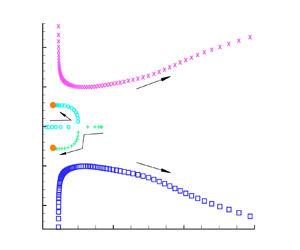
  $Oh_2=0.001$, the viscosity is so low that the vorticity is basically confined within the boundary layers. The velocity fields of the modes at the initial time
  $t=0$ are illustrated in figures 6(e) and (f).

Figure 6. (a–d) Distribution of the normalized eigenfunction of the vorticity,  $T/r$, along
  $r$, for the case of a viscous liquid shell,
  $l=2$,
  $a=0.8$. The solid, dashed and dotted lines denote the absolute value, the real part and the imaginary part of the eigenfunction, respectively. The velocity fields of (e) the out-of-phase mode and (f) the in-phase mode at the initial time
  $t=0$.
For a single liquid droplet, the fundamental mode  $l=2$ was found to decay at the lowest rate and dominate in shape oscillations (Chandrasekhar Reference Chandrasekhar1959; Prosperetti Reference Prosperetti1980b; Li et al. Reference Li, Yin and Yin2020). What about a liquid shell? Figure 7 represents the comparison between the first four modes
  $l=2$, 3, 4 and 5. As shown in the figure, for the higher-order modes
  $l>2$, there are two oscillation patterns as well: the in-phase (blue curves) and the out-of-phase (red curves), which behave similarly to those of
  $l=2$ but with higher damping rates. As a result, for a liquid shell, the mode
  $l=2$ is still dominant. The damping rates of the higher-order modes also bifurcate into two aperiodic branches when
  $Oh_2$ exceeds a critical value. The in-phase mode of
  $l=2$ possesses the widest interval of
  $Oh_2$ for periodic oscillations, as shown in figure 7(b). In the neighbourhood of
  $Oh_2=0$, as
  $Oh_2$ goes away from zero, the angular frequency of the in-phase mode exhibits a sharp descent for all
  $l$ values, possibly owing to the boundary-layer effects caused by viscosity. Accordingly, the inviscid solution overestimates the frequency of oscillation at small values of
  $Oh_2$ to a certain extent. In figure 7(c), the deviation of the phase difference from
  $0^\circ$ or
  $180^\circ$ becomes greater as
  $l$ increases. At the upper aperiodic branch of the out-of-phase mode, the transition to the in-phase mode does not occur for
  $l>2$.

Figure 7. Dependence of (a) the damping rate  $\textrm {Re}(\omega )$, (b) the angular frequency
  $|\textrm {Im}(\omega )|$ and (c) the phase difference
  $\varTheta$ on the Ohnesorge number of the shell
  $Oh_2$, for the case of a viscous liquid shell,
  $l=2$ (solid), 3 (dotted), 4 (short dashed) and 5 (long dashed),
  $a=0.8$. Blue curves, the in-phase mode; red curves, the out-of-phase mode. The insets in panels (b) and (c) show the details at small values of
  $Oh_2$.
3.2. Oscillations of a viscous compound droplet in a vacuum
Setting the values of  $\rho _{r3}$ and
  $\mu _{r3}$ to zero, the eigenvalue problem (2.39) reduces to that for the case of a viscous compound droplet in a vacuum or in a gas of negligible hydrodynamic effects. In this case, six non-dimensional parameters are involved, i.e. the polar wavenumber
  $l$, the Ohnesorge number of the shell
  $Oh_2$, the radius ratio
  $a$, the core to shell density ratio
  $\rho _{r1}$, the core to shell viscosity ratio
  $\mu _{r1}$ and the inner to outer interfacial tension ratio
  $\gamma _r$. The calculation results show that the fundamental mode
  $l=2$ is the dominant one. The parameters
  $Oh_2$ and
  $a$ affect the mode
  $l=2$ in the same way as in the shell case. So, in the following, we focus on the effect of the other three parameters, i.e.
  $\rho _{r1}$,
  $\mu _{r1}$ and
  $\gamma _r$, on the oscillation of a compound droplet in a vacuum.
The effect of the core to shell density ratio  $\rho _{r1}$ on the oscillation of a compound droplet in a vacuum is shown in figures 8 and 9 for
  $Oh_2=1$ and 0.001, respectively, where a wide range of
  $\rho _{r1}$, i.e.
  $\rho _{r1}\in [10^{-2}, 10^2]$, is explored. The core to shell viscosity ratio
  $\mu _{r1}$ is fixed to zero, that is, the core fluid is inviscid. In such a case, the viscosity of the shell is the only factor responsible for the decay of oscillations. At the moderate Ohnesorge number
  $Oh_2=1$, the in-phase mode remains oscillatory as
  $\rho _{r1}$ varies, whereas the out-of-phase mode remains aperiodic without oscillation, as shown in figure 8(a). As
  $\rho _{r1}$ increases, both the damping rate and the angular frequency of the in-phase mode decrease monotonically, see figure 8(b). The increase in
  $\rho _{r1}$ brings more energy to the damped system and, as a result, decelerates the decay of oscillations. However, with the increase in
  $\rho _{r1}$, the droplet becomes heavier and its oscillation is slowed down. The phase difference
  $\varTheta$ of the in-phase mode first decreases and then increases with
  $\rho _{r1}$, as shown in figure 8(c). At small and moderate values of
  $\rho _{r1}$,
  $\varTheta$ remains quite small (
 ${<}5^\circ$) and the inner and outer interfaces of the compound droplet are well coupled. The amplitude ratio
  $\varLambda$, also shown in figure 8(c), remains larger than unity as
  $\rho _{r1}$ varies, which indicates that the inner interface is a major source of vorticity.

Figure 8. (a) Variation of the first four eigenvalues with the core to shell density ratio  $\rho _{r1}$ in the complex frequency plane (
 $\square$ and
  $\times$, the two eigenvalues of the in-phase mode;
  $\circ$ and
  $\bigtriangledown$, the two eigenvalues of the out-of-phase mode), (b) the damping rate
  $\textrm {Re}(\omega )$ (solid) and the angular frequency
  $|\textrm {Im}(\omega )|$ (dashed) and (c) the amplitude ratio
  $\varLambda$ (solid) and the phase difference
  $\varTheta$ (dashed) of the in-phase mode versus
  $\rho _{r1}$ for the case of a compound droplet in a vacuum,
  $l=2$,
  $Oh_2=1$,
  $a=0.8$,
  $\mu _{r1}=0$,
  $\gamma _{r}=1$. In panel (a), the filled circles are the four eigenvalues for the case of a viscous liquid shell in a vacuum and the arrows indicate the direction of
  $\rho _{r1}$ increasing.

Figure 9. (a) Variation of the first four eigenvalues with the core to shell density ratio  $\rho _{r1}$ in the complex frequency plane (
 $\square$ and
  $+$, the two eigenvalues of the in-phase mode;
  $\circ$ and
  $\bigtriangledown$, the two eigenvalues of the out-of-phase mode), (b) the damping rate
  $\textrm {Re}(\omega )$ (short dashed, in-phase; dotted, out-of-phase) and the angular frequency
  $|\textrm {Im}(\omega )|$ (dash-dotted, in-phase; long dashed, out-of-phase) and (c) the amplitude ratio
  $\varLambda$ (short dashed, in-phase; dotted, out-of-phase) and the phase difference
  $\varTheta$ (dash-dotted, in-phase; long dashed, out-of-phase) versus
  $\rho _{r1}$, for the case of a compound droplet in a vacuum,
  $l=2$,
  $Oh_2=0.001$,
  $a=0.8$,
  $\mu _{r1}=0$,
  $\gamma _{r}=1$. In panel (a), the filled circles are the four eigenvalues for the case of a viscous liquid shell in a vacuum and the arrows indicate the direction of
  $\rho _{r1}$ increasing.
The case of small Ohnesorge number is another scenario. As shown in figures 9(a) and 9(b), at  $Oh_2=0.001$, both the in-phase and out-of-phase modes undergo periodic oscillations. Moreover, the damping rate of either mode is remarkably small, owing to the low viscosity. The angular frequency of the in-phase mode is always larger than that of the out-of-phase mode. In addition, interestingly, when
  $\rho _{r1}$ exceeds a cutoff value (approximately 35), the out-of-phase mode disappears. According to the tendency illustrated in figure 9(c), as
  $\rho _{r1}$ approaches the cutoff value, the amplitude ratio
  $\varLambda$ of the out-of-phase mode ascends rapidly and tends to infinity. From a physical point of view, at large values of
  $\rho _{r1}$, the dense core liquid carries a lot of kinetic energy, part of which is transformed into potential energy at the inner interface and results in a large amplitude of oscillation there. Then, the interfacial potential energy is released to sustain the vorticity field and dissipation inside the shell. However, at small Ohnesorge numbers such as 0.001, the effect of viscosity is confined within the boundary layers, and for the out-of-phase mode, with the desperately small damping rate and frequency of oscillation, the potential energy accumulated at the inner interface cannot be released in time to diminish the large amplitude of the inner interface. Ultimately, the out-of-phase mode collapses and disappears. The phase difference of either mode remains close to
  $0^\circ$ or
  $180^\circ$ within the range of
  $\rho _{r1}$ explored, owing to the low viscosity of the system.
The effect of the core to shell viscosity ratio  $\mu _{r1}$ on the damping rate
  $\textrm {Re}(\omega )$ and the angular frequency
  $|\textrm {Im}(\omega )|$ of the in-phase mode is shown in figure 10(a), where the Ohnesorge number
  $Oh_2$ is fixed to a moderate value 1. The out-of-phase mode is not diagrammed for it is aperiodic. Clearly, there exists a critical value of
  $\mu _{r1}$ (approximately
  $1.1$), beyond which the in-phase mode turns aperiodic and bifurcates into two branches. The features of these two aperiodic branches are analogous to those shown in figure 3. Before the bifurcation, the in-phase mode is oscillatory, with the damping rate increasing and the angular frequency decreasing monotonically with increasing
  $\mu _{r1}$. The viscosity of the core seems to affect the in-phase mode in the same way as the viscosity of the shell. Defining the Ohnesorge number of the core as
  $Oh_1=\mu _1/\sqrt {\rho _1\gamma _1R_1}=\mu _{r1}Oh_2/\sqrt {\rho _{r1}\gamma _ra}$, the border between oscillation and no-oscillation in the
  $Oh_1$–
 $Oh_2$ plane is plotted in figure 10(b) for the in-phase mode, where the crosses denote data points and the curve is the fitted result. The border is almost linear, except in the neighbourhood of zero
  $Oh_2$. Below, it is the domain in which the in-phase mode experiences periodic oscillations during its decay and above it, the mode is overdamped. In figure 10(c), for the moderate
  $Oh_2=1$ and
  $\mu _{r1}=1$, the vorticity penetrates deep into both the shell and the core. The velocity field of the in-phase mode at the initial time is shown in figure 10(d).

Figure 10. Influence of the core to shell viscosity ratio  $\mu _{r1}$ on the in-phase mode of a viscous compound droplet in a vacuum,
  $l=2$,
  $a=0.8$,
  $\rho _{r1}=1$,
  $\gamma _r=1$. (a) The damping rate
  $\textrm {Re}(\omega )$ (dotted and dashed) and the angular frequency
  $|\textrm {Im}(\omega )|$ (dash-dotted) versus
  $\mu _{r1}$,
  $Oh_2=1$. (b) The domains in the
  $Oh_1$–
 $Oh_2$ plane. (c) The normalized eigenfunction of the vorticity,
  $T/r$, along
  $r$,
$r$,  $Oh_2=1$,
  $\mu _{r1}=1$. Solid, the absolute value; dashed, the real part; dotted, the imaginary part. (d) The velocity field of the in-phase mode at the initial time
  $t=0$.
The effect of the interfacial tension coefficient ratio  $\gamma _r$ on the in-phase mode is illustrated in figure 11, where
  $\gamma _r$ ranges from 0.2 to 5. The case of moderate viscosities (
 $Oh_2=1$ and
  $\mu _{r1}=1$) is examined, in which the out-of-phase mode remains aperiodic and hence is not plotted in the figure. As shown in figure 11(a), there exists a critical value of
  $\gamma _r$ (
 ${\approx }0.7$), below which the in-phase mode becomes aperiodic with zero frequency of oscillation and, moreover, it bifurcates into two branches. The damping rate of the upper branch increases with decreasing
  $\gamma _r$, while the damping rate of the lower branch decreases. Physically, interfacial tension serves as a restoring force that induces periodic oscillations of a droplet. When
  $\gamma _r$ is smaller than the critical value, interfacial tension is not strong enough to support oscillations of the droplet any more. In experiments, to guarantee that a viscous compound droplet undergoes periodic oscillations, the interfacial tensions need to be sufficiently large. Beyond the critical
  $\gamma _r$, the damping rate of the in-phase mode is little influenced by
  $\gamma _r$, but its oscillation frequency increases remarkably with
  $\gamma _r$. In figure 11(b), both the amplitude ratio
  $\varLambda$ and the phase difference
  $\varTheta$ of the in-phase mode increase with
  $\gamma _r$, which reflects the positive effect of interfacial tension on shape oscillations. Within the range of
  $\gamma _r$ explored, the phase difference remains below
  $3^\circ$, which indicates that varying
  $\gamma _r$ damages little the coupling between the interfaces.

Figure 11. Influence of the interfacial tension coefficient ratio  $\gamma _{r}$ on (a) the damping rate
  $\textrm {Re}(\omega )$ (dotted and dashed) and the angular frequency
  $|\textrm {Im}(\omega )|$ (dash–dotted) and (b) the amplitude ratio
  $\varLambda$ (dotted and dashed) and the phase difference
  $\varTheta$ (dash–dotted) of the in-phase mode of a viscous compound droplet in a vacuum,
  $l=2$,
  $Oh_2=1$,
  $a=0.8$,
  $\rho _{r1}=1$,
  $\mu _{r1}=1$.
3.3. Oscillations of a viscous compound droplet immersed in a viscous host fluid
In the general case of a viscous compound droplet immersed in a viscous host fluid, there are in total eight non-dimensional parameters. Six of them ( $l$,
$l$,  $Oh_2$,
  $a$,
$a$,  $\rho _{r1}$,
  $\mu _{r1}$,
  $\gamma _r$) are identical to those in the case of a compound droplet in a vacuum, and the other two, i.e. the host to shell density ratio
  $\rho _{r3}$ and the host to shell viscosity ratio
  $\mu _{r3}$, are related to the properties of the host fluid. In this subsection, we mainly examine the effect of the host fluid on the oscillation behaviour of the compound droplet by varying the value of
  $\rho _{r3}$ or
  $\mu _{r3}$. Only the results for the fundamental mode
  $l=2$ are presented.
Setting  $\mu _{r3}$ to zero (the host fluid is inviscid), the effect of
  $\rho _{r3}$ on the oscillation of the compound droplet is studied first. The results are represented in figures 12 and 13 for
  $Oh_2=1$ and
  $0.001$, respectively, where
  $\rho _{r3}$ ranges from
  $10^{-2}$ to
  $10^2$. As shown in figure 12(a), at the moderate Ohnesorge number
  $Oh_2=1$, the out-of-phase mode remains aperiodic with
  $\textrm {Im}(\omega )$ equal to zero and its damping rate is little influenced by
  $\rho _{r3}$. Differently, within the range of
  $\rho _{r3}$ explored, the in-phase mode is always oscillatory. The damping rate of the in-phase mode decreases monotonically with
  $\rho _{r3}$ increasing, which indicates that the host fluid serves as an energy supply to slow down the decay of oscillations. The oscillation frequency of the in-phase mode first increases and then decreases as
  $\rho _{r3}$ increases; the maximum is located around
  $\rho _{r3}=1$, see figure 12(b). Clearly, one of the eigenvalues of the aperiodic out-of-phase mode (the one denoted by the symbol
  $\times$ in figure 12a) possesses the smallest damping rate, and therefore is dominant in the decay of perturbations under natural conditions. In such a case, excitations of in-phase type need to be imposed on the system at the initial time for the observation of shape oscillations in experiments. In figure 12(c), the phase difference
  $\varTheta$ of the in-phase mode increases with
  $\rho _{r3}$. When
  $\rho _{r3}$ is small or moderate (
 $\rho _{r3}<10$),
  $\varTheta$ remains tolerably below
  $5^\circ$. However, at larger
  $\rho _{r3}$,
  $\varTheta$ may increase to considerably large values so that the in-phase mode cannot even be said to be approximately in phase. Within the range of
  $\rho _{r3}$ explored, the amplitude ratio
  $\varLambda$ of the in-phase mode basically remains larger than unity, which indicates that the inner interface is the major source of vorticity. However, the tendency suggests that at sufficiently large values of
  $\rho _{r3}$ (i.e.
  $\rho _{r3}\sim O(10^2)$ or even larger, which may go beyond the physical realistic),
  $\varLambda$ drops below unity and the much denser host fluid becomes an important energy supply.

Figure 12. (a) Variation of the first four eigenvalues with the host to shell density ratio  $\rho _{r3}$ in the complex frequency plane (
 $\square$ and
  $+$, the two eigenvalues of the in-phase mode;
  $\circ$ and
  $\times$, the two eigenvalues of the out-of-phase mode; the arrows indicate the direction of
  $\rho _{r3}$ increasing). (b) The damping rate
  $\textrm {Re}(\omega )$ (dashed) and the angular frequency
  $|\textrm {Im}(\omega )|$ (dotted) and (c) the amplitude ratio
  $\varLambda$ (dashed) and the phase difference
  $\varTheta$ (dotted) of the in-phase mode versus
  $\rho _{r3}$, for the case of a viscous compound droplet immersed in an inviscid host fluid,
  $l=2$,
  $Oh_2 = 1$,
  $a=0.8$,
  $\rho _{r1}=1$,
  $\mu _{r1}=1$,
  $\gamma _r=1$,
  $\mu _{r3}=0$.

Figure 13. (a) Variation of the first four eigenvalues with the host to shell density ratio  $\rho _{r3}$ in the complex frequency plane (
 $\square$ and
  $+$, the two eigenvalues of the in-phase mode;
  $\circ$ and
  $\bigtriangledown$, the two eigenvalues of the out-of-phase mode; the arrows indicate the direction of
  $\rho _{r3}$ increasing), (b) the damping rate
  $\textrm {Re}(\omega )$ (short dashed, in-phase; dotted, out-of-phase) and the angular frequency
  $|\textrm {Im}(\omega )|$ (dashed–dotted, in-phase; long dashed, out-of-phase) and (c) the amplitude ratio
  $\varLambda$ (short dashed, in-phase; dotted, out-of-phase) and the phase difference
  $\varTheta$ (dashed–dotted, in-phase; long dashed, out-of-phase) versus
  $\rho _{r3}$, for the case of a viscous compound droplet immersed in an inviscid host fluid,
  $l=2$,
  $Oh_2 = 0.001$,
  $a=0.8$,
  $\rho _{r1}=1$,
  $\mu _{r1}=1$,
  $\gamma _r=1$,
  $\mu _{r3}=0$.
At the small Ohnesorge number  $Oh_2 = 0.001$, both the in-phase and the out-of-phase modes oscillate periodically, and moreover, they are fairly long-lived for their small damping rates, as shown in figure 13. The damping rate of the in-phase mode increases with
  $\rho _{r3}$, a trend different from for the moderate value
  $Oh_2 = 1$, as shown in figure 12. The angular frequency of either mode is decreased by
  $\rho _{r3}$. When
  $\rho _{r3}$ exceeds a cutoff value of approximately
  $66$, the out-of-phase mode disappears, as in the case of large
  $\rho _{r1}$ illustrated in figure 9 and the mechanism behind it is essentially the same. This time, the dense host fluid transfers too much energy to the outer interface and, as a consequence, the amplitude of the outer interface becomes extremely large and the amplitude ratio
  $\varLambda$ becomes extremely small (tends to zero), as shown in figure 13(c); however, the viscosity of the shell fluid is so low that the potential energy at the outer interface fails to be released in time and the amplitude of the outer interface cannot be lowered to a normal level. In one word, this phenomenon, i.e. the disappearance of the out-of-phase mode at large core-to-shell or host-to-shell density ratios, may be attributed to the failure of the slightly viscous shell in releasing interfacial energy. Anyway, there is no need to pay much attention to this phenomenon, for it occurs only at very large density contrasts that seem to be physically unrealistic. The amplitude ratio of the in-phase mode also behaves unusually, which increases continuously and becomes remarkably large when
  $\rho _{r3}$ goes beyond 10. However, note that at large values of
  $\rho _{r3}$, the in-phase mode decays faster than the out-of-phase mode and the latter is the dominant one. At small values of the Ohnesorge numbers
  $Oh_1$ and
  $Oh_2$, increasing
  $\rho _{r3}$ seems to favour the out-of-phase mode (before it vanishes) in shape oscillations of the compound droplet. Owing to small viscosities of the fluids, the phase difference of either mode remains close to
  $0\,^\circ$ or
  $180^\circ$, regardless of the value of
  $\rho _{r3}$.
For an unbounded viscous fluid field, there commonly exists a continuous spectrum (Prosperetti Reference Prosperetti1980b; Schmid & Henningson Reference Schmid and Henningson2001). In this problem, the continuous spectrum is a vertical straight line located at the positive semi-axis of  $\textrm {Re}(\omega )$, as shown in figure 14(a). Note that it is discretized because of the truncation of the host fluid domain when applying the spectral method. Because all the modes belonging to the continuous spectrum are aperiodic and decay without oscillation, it is of no interest in this study. Well, one thing about this aperiodic continuous spectrum is worthy to be mentioned. In the calculation, it is found that the eigenvalues on the continuous spectrum which are smaller than some critical value all belong to the out-of-phase mode, and the eigenvalues that are larger than this critical value belong to the in-phase mode, similar to the discrete spectrum, as illustrated in figure 2 for the shell case.

Figure 14. Influence of the host to shell viscosity ratio  $\mu _{r3}$ on the oscillation of a viscous compound droplet immersed in a viscous host fluid,
  $l=2$,
  $Oh_2=1$,
  $a=0.8$,
  $\rho _{r1}=1$,
  $\mu _{r1}=1$,
  $\gamma _r=1$,
  $\rho _{r3}=1$. (a) Spectrum of eigenvalues,
  $\mu _{r3}=1$. (b) Variation of the eigenvalues with
  $\mu _{r3}$ in the complex frequency plane, where the arrows indicate the direction of
  $\mu _{r3}$ increasing. (c) The damping rate
  $\textrm {Re}(\omega )$ (
 $\circ$) and the angular frequency
  $|\textrm {Im}(\omega )|$ (
 $\times$) and (d) the amplitude ratio
  $\varLambda$ (
 $\square$) and the phase difference
  $\varTheta$ (
 $+$) of the in-phase mode versus
  $\mu _{r3}$.
The two discrete eigenvalues with non-zero imaginary parts, denoted by the filled squares in figure 14(a), belong to the in-phase mode. In the case of moderate viscosities ( $Oh_2=1, \mu _{r1}=1, \mu _{r3}=1$) considered, the out-of-phase mode is aperiodic with zero angular frequency. The variation of the two discrete eigenvalues with the host to shell viscosity ratio
  $\mu _{r3}$ is illustrated in figure 14(b), where
  $\mu _{r3}$ ranges from 0 to 10. Apparently, both the damping rate
  $\textrm {Re}(\omega )$ and the angular frequency
  $|\textrm {Im}(\omega )|$ of the in-phase mode are decreased by increasing
  $\mu _{r3}$. The trend can also be seen in figure 14(c). The viscosity of the host fluid tends to slow down the decay of oscillations, different from the effect of the viscosity of the core or the shell illustrated in figures 3 or 10. In practice, the viscosity of the host fluid has a dual effect on the oscillation of the system. On one hand, it causes energy dissipation and tends to enhance the decay of perturbations; on the other hand, it prompts the diffusion of vorticity and tends to suppress the decay of perturbations (Prosperetti Reference Prosperetti1980b; Li et al. Reference Li, Yin and Yin2020). For the values of the non-dimensional parameters considered in figure 14, it appears that the second mechanism overwhelms the first. Nevertheless, it does not mean that a higher viscosity of the host fluid will result in the compound droplet oscillating better, for the frequency of oscillation can be significantly diminished by
  $\mu _{r3}$. As shown in figure 14(c), when
  $\mu _{r3}$ exceeds 2, the angular frequency
  $|\textrm {Im}(\omega )|$ decreases to small values very close to zero and basically the in-phase mode can be regarded as an overdamped mode.
Define the Ohnesorge number of the host fluid as  $Oh_3=\mu _3/\sqrt {\rho _3\gamma _2R_2}=\mu _{r3}Oh_2/\sqrt {\rho _{r3}}$, and the dual effect of the viscosity of the host fluid is further demonstrated in figure 15, where the variation of the damping rate
  $\textrm {Re}(\omega )$ and the angular frequency
  $|\textrm {Im}(\omega )|$ of the in-phase mode with
  $Oh_3$ is diagrammed for several values of the Ohnesorge number of the shell
  $Oh_2$. As shown in figure 15(a), at different values of
  $Oh_2$, the viscosity of the host fluid influences the damping rate of the in-phase mode in different ways. At relatively large values of
  $Oh_2$ such as 1 and 1.5,
  $\textrm {Re}(\omega )$ decreases monotonically with
  $Oh_3$ increasing, which suggests that when the viscosity of the shell is sufficiently high, the suppression effect of the viscosity of the host on the decay of perturbations is more pronounced. In contrast, at relatively small values of
  $Oh_2$ such as 0.1, 0.2 and 0.5, as
  $Oh_3$ increases,
  $\textrm {Re}(\omega )$ first increases and then decreases. That is, when the viscosities of both the shell and the host are low, the viscosity of the host tends to accelerate the decay of oscillations; differently, when the viscosity of the host itself is sufficiently high, its effect of promoting vorticity diffusion inside fluid bulk is more pronounced and, as a result, the decay of perturbations is slowed down. In addition to the Ohnesorge number of the shell
  $Oh_2$, the other non-dimensional parameters may influence the role the viscosity of the host plays as well, which are not examined here.

Figure 15. Variation of (a) the damping rate  $\textrm {Re}(\omega )$ and (b) the angular frequency
  $|\textrm {Im}(\omega )|$ of the in-phase mode with the Ohnesorge number of the host fluid
  $Oh_3$ for various values of the Ohnesorge number of the shell fluid
  $Oh_2$. The case of a viscous compound droplet immersed in a viscous host fluid,
  $l=2$,
  $a=0.8$,
  $\rho _{r1}=1$,
  $\mu _{r1}=1$,
  $\gamma _r=1$,
  $\rho _{r3}=1$.
As a matter of fact, in the presence of the unbounded viscous host fluid, the viscosity of the shell fluid also exhibits a duel effect on shape oscillations of the compound droplet. As outlined previously, when the host fluid is absent, increasing the viscosity of the shell fluid only leads to the increase in the damping rate of the in-phase mode within the interval of  $Oh_2$ for periodic oscillations. The presence of the host fluid may trigger the second effect of the viscosity of the shell, that is, suppressing the decay of oscillations by transporting energy. As shown in figure 15(a), at moderate or relatively large values of
  $Oh_3$, say
  $Oh_3=1$, the damping rate
  $\textrm {Re}(\omega )$ of the in-phase mode decreases monotonically as
  $Oh_2$ increases. Differently, when the viscosity of the host is low, say
  $Oh_3=0.1$, the damping rate increases first and then decreases with increasing
  $Oh_2$. The dual effect of the viscosity of the shell can be more clearly seen in figure 17(a) in the next subsection. Note that, in the presence of a viscous host fluid, the damping rate bifurcates no more. The in-phase mode maintains periodic oscillations no matter how large
  $Oh_2$ is. Moreover, the in-phase mode remains oscillatory for all values of
  $Oh_3$. Nevertheless, as shown in figures 15(b) and 17(b), as
  $Oh_2$ or
  $Oh_3$ increases from zero, the frequency of oscillation decreases rapidly and almost becomes zero at finite values of
  $Oh_2$ or
  $Oh_3$, for which the in-phase mode is almost aperiodic.
For the case considered in figure 14, the amplitude ratio  $\varLambda$ increases with
  $\mu _{r3}$, while the phase difference
  $\varTheta$ first increases and then decreases. Note that in figures 14(c) and 14(d),
  $\textrm {Re}(\omega )$,
  $|\textrm {Im}(\omega )|$,
  $\varLambda$ and
  $\varTheta$ all appear intermittently at large values of
  $\mu _{r3}$. In the calculation, with the removal of the continuous spectrum which is aperiodic with
  $\textrm {Im}(\omega )$ equal to zero, any eigenvalues whose imaginary parts are smaller than 0.001 are filtered off, which includes those of the discrete spectrum (when
  $|\textrm {Im}(\omega )|<0.001$, the initial disturbance is considered to be overdamped). In addition, in figure 14(d), at large values of
  $\mu _{r3}$, the phase difference
  $\varTheta$ unusually forms a queue of peaks. The peaks appear periodically and regularly, and we are not sure if they are caused by numerical errors. Anyway, they only appear when the frequency of oscillation drops down to nearly zero, of little importance to shape oscillations of the system.
The eigenfunction of the vorticity,  $T/r$, and the velocity field of the in-phase mode at the initial time are illustrated in figures 16(a) and 16(b), respectively. At the moderate viscosity of the host, the vorticity penetrates quite deep into the fluid bulk. The flow field is analogous to that of a quadrupole, because the polar wavenumber
  $l$ is equal to 2.

Figure 16. (a) The eigenfunction of the vorticity,  $T/r$, along
  $r$ (solid, the absolute value; dashed, the real part; dotted, the imaginary part) and (b) the velocity field of the in-phase mode at the initial time
  $t=0$, for the case of a viscous compound droplet immersed in a viscous host fluid,
  $l=2$,
  $Oh_2=1$,
  $a=0.8$,
  $\rho _{r1}=1$,
  $\mu _{r1}=1$,
  $\gamma _r=1$,
  $\rho _{r3}=1$,
  $\mu _{r3}=1$.
3.4. Thin shell approximation
The thin shell approximation of the three-fluid system, in which the thickness of the shell is much smaller than the outer radius of the shell, i.e.  $\epsilon =1-a\ll 1$, is of particular interest in some processing techniques such as coating and encapsulation and also in modelling biological cells with membranes. The characteristic equation for this limiting case is derived in Appendix D and the supplementary material. It is found that the in-phase mode is dominant. The inner and outer interfaces of the compound droplet oscillate perfectly in phase with equal amplitude. Moreover, the hydrodynamic effect of the shell is neglected to the leading order, and the system behaves like a single droplet consisting only of the core liquid but bearing capillary pressures from both the inner and outer interfaces, as found in the case of overdamped compound droplets of highly viscous fluids (Landman Reference Landman1985). In the study of the thin annular limiting case of a cylindrical compound jet, it was also found that the stretching (in-phase) mode is dominant and the compound jet behaves like a single jet with tension equal to the sum of the two interfacial tensions (Chauhan et al. Reference Chauhan, Maldarelli, Papageorgiou and Rumschitzki2000). With an extra interfacial tension, a liquid droplet encapsulated by a thin liquid shell oscillates at a higher frequency and a smaller damping rate compared with the case of no shell, which is an advantage in mixing, mass/heat transfer and other potential applications. The characteristic equation for the thin shell limiting case is obtained by setting the second determinant in (D1) equal to zero. Here we write it in a more compact form following Prosperetti (Reference Prosperetti1980b),
 \begin{align}
&\frac{\omega^2_0}{\omega^2}\nonumber\\ &\quad
={-}1+\frac{\left[(2~l+1)\mathscr{P}_1+2l(l+2)\left(\dfrac{\mu_{r3}}{\mu_{r1}}-1\right)\right]
\left[(2l+1)\dfrac{\mu_{r3}}{\mu_{r1}}\mathscr{Q}_3-2(l-1)(l+1)\left(\dfrac{\mu_{r3}}{\mu_{r1}}
-1\right)\right]}{z^2_1\left(\dfrac{\rho_{r3}}{\rho_{r1}}l+l+1\right)\left[\mathscr{P}_1+
\dfrac{\mu_{r3}}{\mu_{r1}}\mathscr{Q}_3
+2\left(\dfrac{\mu_{r3}}{\mu_{r1}}-1\right)\right]},
\end{align}
\begin{align}
&\frac{\omega^2_0}{\omega^2}\nonumber\\ &\quad
={-}1+\frac{\left[(2~l+1)\mathscr{P}_1+2l(l+2)\left(\dfrac{\mu_{r3}}{\mu_{r1}}-1\right)\right]
\left[(2l+1)\dfrac{\mu_{r3}}{\mu_{r1}}\mathscr{Q}_3-2(l-1)(l+1)\left(\dfrac{\mu_{r3}}{\mu_{r1}}
-1\right)\right]}{z^2_1\left(\dfrac{\rho_{r3}}{\rho_{r1}}l+l+1\right)\left[\mathscr{P}_1+
\dfrac{\mu_{r3}}{\mu_{r1}}\mathscr{Q}_3
+2\left(\dfrac{\mu_{r3}}{\mu_{r1}}-1\right)\right]},
\end{align}
where  $\omega _0$ is the frequency of oscillation in the inviscid case,
 $$\begin{gather} \omega^2_0 = \frac{(\gamma_r+1)(l-1)l(l+1)(l+2)}{\dfrac{\mu_{r3}}{\mu_{r1}}l+l+1}, \end{gather}$$
 $$\begin{gather}z_1=\sqrt{\frac{\rho_{r1}\omega}{\mu_{r1}Oh_2}}, \quad z_3=\sqrt{\frac{\rho_{r3}\omega}{\mu_{r3}Oh_2}}, \end{gather}$$
 $$\begin{gather}\mathscr{P}_1=z_1\frac{\textrm{J}_{l+{1}/{2}}(z_1)}{\textrm{J}_{l+{3}/{2}}(z_1)}, \quad \mathscr{Q}_3=z_3\frac{H^{(1)}_{l+{1}/{2}}(z_3)}{H^{(1)}_{l-{1}/{2}}(z_3)}, \end{gather}$$
where  $\textrm {J}(\cdot )$ and
  $H^{(1)}(\cdot )$ are the Bessel function of the first kind and the Hankel function of the first kind, respectively, and the corresponding subscripts denote their orders.
The accuracy of the thin shell approximation is examined in figure 17, where the dotted curves are the results for the three-fluid system obtained with the aid of the spectral method and the solid curves are the results of the thin shell approximation obtained by solving the characteristic equation (3.1). As shown in figures 17(a) and 17(b), as the radius ratio  $a$ increases from 0.7 to 0.99, both the damping rate
  $\textrm {Re}(\omega )$ and the angular frequency
  $|\textrm {Im}(\omega )|$ of the in-phase mode of the three-fluid system approach the values estimated by the thin shell approximation. Moreover, as
  $a$ increases, the amplitude ratio
  $\varLambda$ approaches unity, see figure 17(c), which indicates that the inner and outer interfaces possess almost equal amplitudes at large values of
  $a$; meanwhile, the phase difference
  $\varTheta$ approaches zero, see figure 17(d), which indicates that with the decrease in the thickness of the shell, the interfaces oscillate more and more in phase, consistent with the prediction of the thin shell approximation. Generally, the thin shell approximation well predicts the oscillation characteristics of the three-fluid system when
  $a$ is near 1, although it may underestimate the damping rate and the frequency of oscillation owing to the neglect of the hydrodynamic effect of the shell fluid.

Figure 17. Comparison of the three-fluid case with the thin shell approximation. (a) The damping rate  $\textrm {Re}(\omega )$, (b) the angular frequency
  $|\textrm {Im}(\omega )|$, (c) the amplitude ratio
  $\varLambda$ and (d) the phase difference
  $\varTheta$ versus the Ohnesorge number of the shell
  $Oh_2$, for distinct values of the radius ratio
  $a$ (the dotted curves), where
  $l=2$,
  $\rho _{r1}=1$,
  $\mu _{r1}=1$,
  $\gamma _r=1$,
  $\rho _{r3}=1$,
  $\mu _{r3}=1$. The arrows indicate the direction of
  $a$ increasing. The solid curves in panels (a) and (b) are the results of the thin shell approximation
  $a\rightarrow 1$.
4. Conclusion
In this paper, the small-amplitude shape oscillation of a viscous compound droplet suspended in a viscous host fluid is investigated. A generalized eigenvalue equation is built, and the damping rate, the angular frequency and the other quantities characterizing the oscillation behaviour of the droplet are solved numerically with the aid of the spectral method. The effects of the relevant non-dimensional parameters on shape oscillations of the droplet are examined successively by considering three cases, i.e. a viscous shell in a vacuum, a viscous compound droplet in a vacuum and a viscous compound droplet suspended in a viscous host fluid.
It is found that the fundamental mode  $l=2$ is dominant in shape oscillations of the compound droplet. For
  $l=2$ (also for higher-order modes
  $l>2$), there exist two oscillatory modes, i.e. the in-phase mode and the out-of-phase mode. The in-phase mode dominates oscillations, except when the viscosities of the fluids are very small. Owing to viscosity, the inner and outer interfaces of the compound droplet do not oscillate strictly in the same direction in the in-phase mode or oscillate in totally opposite directions in the out-of-phase mode. Furthermore, the coupling between the interfaces is greatly influenced by the thickness of the shell. Generally, a thicker shell leads to the phase difference between the interfaces deviating more from
  $0^\circ$ or
  $180^\circ$. In contrast, in the thin shell limit, the interfaces oscillate nicely in phase, the hydrodynamic effect of the shell is of secondary importance and the system behaves like a single droplet of the core fluid immersed in the host fluid but with the tensions of both interfaces.
In the absence of the host fluid, the spectrum in the complex frequency plane is a discrete one. Normally, two of the eigenvalues belong to the out-of-phase mode and the rest belong to the in-phase mode. We focus on the four eigenvalues with the smallest real parts, which decay the slowest and therefore determine the oscillation behaviour of the compound droplet. Among these four eigenvalues, two are of the in-phase mode and the other two of the out-of-phase mode (at high viscosities, the transition from the out-of-phase to the in-phase mode may occur on one of the eigenvalues). For either mode, in the absence of a viscous host fluid, the increase in the viscosity of the core or the shell fluid leads to the increase in the damping rate as well as the decrease in the oscillation frequency. When the viscosity increases to a critical value, the transition of a mode from oscillatory to aperiodic decay takes place, and beyond the critical viscosity, the damping rate of a mode bifurcates into an upper branch that decays rapidly and a lower branch that exhibits a feature of the creeping motion of strongly overdamped oscillators. The border between oscillation and no-oscillation is fitted in the plane of the Ohnesorge numbers of the core and the shell,  $Oh_1$ and
  $Oh_2$, for the in-phase mode.
In the presence of the unbounded viscous host fluid, the situation is much more complicated. First, in addition to the discrete spectrum, there exists a continuous spectrum, which occupies the entire non-negative real axis in the complex frequency plane. The eigenvalues on the continuous spectrum belong to either the out-of-phase or the in-phase mode, depending on the eigenvalues being smaller or larger than some critical value. The continuous spectrum corresponds to aperiodic modes, which is of little interest in shape oscillations of the droplet. Second, owing to the viscosity of the host fluid, there exists no such critical value of the Ohnesorge number  $Oh_1$ or
  $Oh_2$ beyond which the transition of the modes from oscillatory to aperiodic decay occurs. The damping rates of the modes bifurcate no more. With the increase in the viscosity of the shell, the oscillation frequency of the mode decreases rapidly but remains larger than zero. When the Ohnesorge number of the host fluid
  $Oh_3$ approaches infinity, the oscillation frequency approaches zero.
The viscosity of the host fluid is found to have a dual effect on the damping rate of the in-phase mode. When the viscosity of the host is small, it mainly causes the dissipation of energy and accelerates the decay of oscillations. In contrast, when it is sufficiently large, its second effect becomes more significant, that is, enhances energy transport and vorticity penetration into fluid bulk, and as a result, the decay of oscillations is slowed. It is also found that the viscosity of the host only exhibits this dual effect when the viscosity of the shell is low. At moderate or high viscosities of the shell, the viscosity of the host just decreases the damping rate of the mode. Notably, in the presence of the viscous host fluid, the viscosity of the shell fluid may also exhibit a similar dual effect on the damping rate of the in-phase mode.
The core-to-shell and host-to-shell density ratios have a great effect on the oscillation characteristics of the compound droplet. When the viscosity of the droplet is moderate or high, only the in-phase mode is oscillatory, and increasing the core-to-shell or host-to-shell density ratio generally leads to the decrease in both the damping rate and the oscillation frequency of the in-phase mode. When the viscosity of the droplet is very low, both the in-phase and out-of-phase modes are oscillatory and the density ratios affect them in different ways. Particularly, increasing the density of the core or host fluid helps the out-of-phase mode to be dominant, but sufficiently large densities of the core or the host may lead to the disappearance of this mode.
Finally, to make the oscillation of the compound droplet possible, the interfacial tension of the inner interface cannot be too small. It is found that decreasing the interfacial tension of the inner interface leads to the decrease in the oscillation frequency of the in-phase mode. Moreover, when the tension is decreased below a critical value, the in-phase mode becomes aperiodic. If naturally an aperiodic mode dominates the decay of perturbations, as in some cases considered in this study, excitations need to be specifically imposed on the compound droplet to observe shape oscillations.
Supplementary material
Supplementary material is available at https://doi.org/10.1017/jfm.2021.981.
Acknowledgements
We thank all the reviewers and the editor for their constructive comments and suggestions.
Funding
This work was supported by the National Natural Science Foundation of China (grant numbers 11772328, 11621202).
Declaration of interests
The authors report no conflict of interest.
Appendix A. About the vector  ${B}$
${B}$

Like the other quantities, the vector  $\boldsymbol {B}$ in (2.14) can be decomposed as
 \begin{equation} \boldsymbol{B}_i=S_i(r)\boldsymbol{e}_rP^m_l(\cos \theta)\exp(\textrm{j}m\varphi-\omega t), \quad i=1, 2, 3, \end{equation}
where  $S(r)$ is the initial amplitude of
  $\boldsymbol {B}$.
Substituting the decomposition (A1) into (2.14) and then (2.14) into (2.13), we get the governing equation for  $S(r)$,
 \begin{equation} \frac{\textrm{d}^2 S_i}{\textrm{d}r^2}-\frac{l(l+1)}{r^2}S_i +\frac{\rho_i\omega}{\mu_i}S_i=0, \quad i=1, 2, 3. \end{equation}
 Considering the boundedness of  $S(r)$ at the origin
  $r=0$ and at infinity, the solution to (A2) is
 $$\begin{gather} S_1 = C_1r^{1/2}\textrm{J}_{l+{1}/{2}}(\vartheta_1r), \end{gather}$$
 $$\begin{gather}S_2 =C_2r^{1/2}\textrm{J}_{l+{1}/{2}}(\vartheta_2r)+C_3r^{1/2}\textrm{Y}_{l+{1/2}}(\vartheta_2r), \end{gather}$$
 $$\begin{gather} S_3=C_4r^{1/2}H^{(1)}_{l+{1}/{2}}(\vartheta_3r), \quad \textrm{if}\ \textrm{Im}(\omega)\neq0, \end{gather}$$
 $$\begin{gather}S_3=C_5r^{1/2}\textrm{J}_{l+{1}/{2}}(\vartheta_3r)+C_6r^{1/2}\textrm{Y}_{l+{1}/{2}}(\vartheta_3r), \quad \textrm{if}\ \textrm{Im}(\omega)=0, \end{gather}$$
where
 \begin{equation} \vartheta_i=\sqrt{\frac{\rho_i \omega}{\mu_i}}, \quad i=1, 2, 3, \end{equation}
where  $\textrm {J}_{l+{1}/{2}}(\cdot )$ and
  $\textrm {Y}_{l+{1}/{2}}(\cdot )$ are, respectively, the Bessel functions of the first and second kinds,
  $H^{(1)}_{l+{1}/{2}}(\cdot )$ is the Hankel function of the first kind with order
  $l+\frac {1}{2}$, and
  $C_1$–
 $C_6$ are the coefficients to be determined by the boundary conditions (2.3a,b)–(2.10). Finally, one finds that the eigenvalue
  $\omega$ can be any real, non-negative number, which forms a continuous spectrum occupying the entire positive real semi-axis in the complex frequency plane. Physically, the continuous spectrum corresponds to purely rotational waves or shear waves (Miller & Scriven Reference Miller and Scriven1968; Prosperetti Reference Prosperetti1980b). Waves of this type cause no interface displacement and are irrelevant to shape oscillations of the droplet. Moreover, owing to the lack of restoring force, these waves are always damped without oscillation.
Appendix B. The characteristic equation for small-amplitude shape oscillations of a viscous compound droplet suspended in a viscous host fluid
Following the method of Chandrasekhar (Reference Chandrasekhar1959), the characteristic equation for small-amplitude shape oscillations of this three-fluid system is derived, which can be expressed in the form of a  $10\times 10$ matrix,
 \begin{align}
\left|\begin{array}{@{}cccccccccc@{}} \omega & 1 & 0 & 0 & 0 & 0
& 0 & 0 & 0 & 0 \\ 0 & 0 & 0 & 0 & 0 & 0 & 0 & 1 & 0 &
\omega \\ 0 & 1 & 0 & R_1^{l-1} & R_1^{-(l+2)} &
R_1^{-{3}/{2}}\kappa_1 & R_1^{-{3}/{2}}\upsilon_1 & 0 & 0 &
0 \\ 0 & 0 & 0 & R_2^{l-1} & R_2^{-(l+2)} &
R_2^{-{3}/{2}}\kappa_2 & R_2^{-{3}/{2}}\upsilon_2 & 1 & 0 &
0 \\ 0 & l+1 & X_6 & (l+1)R_1^{l-1} & -lR_1^{-(l+2)} &
R_1^{-{3}/{2}}H_1 & R_1^{-{3}/{2}}\varPi_1 & 0 & 0 & 0 \\ 0
& 0 & 0 & -(l+1)R_2^{l-1} & lR_2^{-(l+2)} &
-R_2^{-{3}/{2}}H_2 & -R_2^{-{3}/{2}}\varPi_2 & l & Z_6 & 0
\\ 0 & X_5 & X_3 & \bar{\textrm{Y}}_5 & \bar{\textrm{Y}}_7
& \mu_2R_1^{-{3}/{2}}H_3 & \mu_2R_1^{-{3}/{2}}\varPi_3 & 0
& 0 & 0 \\ 0 & 0 & 0 & \bar{\textrm{Y}}_6 &
\bar{\textrm{Y}}_8 & \mu_2R_2^{-{3}/{2}}H_4 &
\mu_2R_2^{-{3}/{2}}\varPi_4 & Z_5 & Z_2 & 0 \\ X_1 & -X_2 &
X_4 & -\bar{\textrm{Y}}_1 & \bar{\textrm{Y}}_3 &
2\mu_2R_1^{-{7}/{2}}H_5 & 2\mu_2R_1^{-{7}/{2}}\varPi_5 & 0
& 0 & 0 \\ 0 & 0 & 0 & \bar{\textrm{Y}}_2 &
-\bar{\textrm{Y}}_4 & -2\mu_2R_2^{-{7}/{2}}H_6 &
-2\mu_2R_2^{-{7}/{2}}\varPi_6 & -Z_1 & Z_3 & Z_4
\end{array} \right|=0, \end{align}
\begin{align}
\left|\begin{array}{@{}cccccccccc@{}} \omega & 1 & 0 & 0 & 0 & 0
& 0 & 0 & 0 & 0 \\ 0 & 0 & 0 & 0 & 0 & 0 & 0 & 1 & 0 &
\omega \\ 0 & 1 & 0 & R_1^{l-1} & R_1^{-(l+2)} &
R_1^{-{3}/{2}}\kappa_1 & R_1^{-{3}/{2}}\upsilon_1 & 0 & 0 &
0 \\ 0 & 0 & 0 & R_2^{l-1} & R_2^{-(l+2)} &
R_2^{-{3}/{2}}\kappa_2 & R_2^{-{3}/{2}}\upsilon_2 & 1 & 0 &
0 \\ 0 & l+1 & X_6 & (l+1)R_1^{l-1} & -lR_1^{-(l+2)} &
R_1^{-{3}/{2}}H_1 & R_1^{-{3}/{2}}\varPi_1 & 0 & 0 & 0 \\ 0
& 0 & 0 & -(l+1)R_2^{l-1} & lR_2^{-(l+2)} &
-R_2^{-{3}/{2}}H_2 & -R_2^{-{3}/{2}}\varPi_2 & l & Z_6 & 0
\\ 0 & X_5 & X_3 & \bar{\textrm{Y}}_5 & \bar{\textrm{Y}}_7
& \mu_2R_1^{-{3}/{2}}H_3 & \mu_2R_1^{-{3}/{2}}\varPi_3 & 0
& 0 & 0 \\ 0 & 0 & 0 & \bar{\textrm{Y}}_6 &
\bar{\textrm{Y}}_8 & \mu_2R_2^{-{3}/{2}}H_4 &
\mu_2R_2^{-{3}/{2}}\varPi_4 & Z_5 & Z_2 & 0 \\ X_1 & -X_2 &
X_4 & -\bar{\textrm{Y}}_1 & \bar{\textrm{Y}}_3 &
2\mu_2R_1^{-{7}/{2}}H_5 & 2\mu_2R_1^{-{7}/{2}}\varPi_5 & 0
& 0 & 0 \\ 0 & 0 & 0 & \bar{\textrm{Y}}_2 &
-\bar{\textrm{Y}}_4 & -2\mu_2R_2^{-{7}/{2}}H_6 &
-2\mu_2R_2^{-{7}/{2}}\varPi_6 & -Z_1 & Z_3 & Z_4
\end{array} \right|=0, \end{align}
where
 \begin{gather} \varUpsilon_1=\frac{\textrm{J}_{l+{3}/{2}}{(\vartheta_1R_1)}}{\textrm{J}_{l+{1}/{2}}(\vartheta_1R_1)},\quad \varUpsilon_2=\frac{H^{(1)}_{l+{3}/{2}}{(\vartheta_3R_2)}}{H^{(1)}_{l+{1}/{2}}(\vartheta_3R_2)}, \end{gather}
 \begin{gather} H_5=(l-1)\kappa_1-\vartheta_2R_1\kappa_3,\quad H_6=(l-1)\kappa_2-\vartheta_2R_2\kappa_4, \end{gather}
 \begin{gather} \varPi_5=(l-1)\upsilon_1-\vartheta_2R_1\upsilon_3,\quad \varPi_6=(l-1)\upsilon_2-\vartheta_2R_2\upsilon_4, \end{gather}
 \begin{gather} \kappa_1=\textrm{J}_{l+{1}/{2}}(\vartheta_2R_1), \quad \kappa_2=\textrm{J}_{l+{1}/{2}}(\vartheta_2R_2), \quad \kappa_3=\textrm{J}_{l+{3}/{2}}(\vartheta_2R_1), \quad \kappa_4=\textrm{J}_{l+{3}/{2}}(\vartheta_2R_2), \end{gather}
 \begin{gather} \upsilon_1=\textrm{Y}_{l+{1}/{2}}(\vartheta_2R_1), \quad \upsilon_2=\textrm{Y}_{l+{1}/{2}}(\vartheta_2R_2), \quad \upsilon_3=\textrm{Y}_{l+{3}/{2}}(\vartheta_2R_1), \quad \upsilon_4=\textrm{Y}_{l+{3}/{2}}(\vartheta_2R_2), \end{gather}
 \begin{gather} H_1=(l+1)\kappa_1-\vartheta_2R_1\kappa_3,\quad H_2=(l+1)\kappa_2-\vartheta_2R_2\kappa_4, \end{gather}
 \begin{gather} H_3=(2l^2-2-\vartheta^2_2R^2_1)\kappa_1+2\vartheta_2R_1\kappa_3, \quad H_4=(2l^2-2-\vartheta^2_2R^2_2)\kappa_2+2\vartheta_2R_2\kappa_4, \end{gather}
 \begin{gather} \varPi_1=(l+1)\upsilon_1-\vartheta_2R_1\upsilon_3,\quad \varPi_2=(l+1)\upsilon_2-\vartheta_2R_2\upsilon_4, \end{gather}
 \begin{gather} \varPi_3=(2l^2-2-\vartheta^2_2R^2_1)\upsilon_1+2\vartheta_2R_1\upsilon_3, \quad \varPi_4=(2l^2-2-\vartheta^2_2R^2_2)\upsilon_2+2\vartheta_2R_2\upsilon_4, \end{gather}
 \begin{gather} X_1=\frac{\gamma_1(l-1)(l+2)}{R^3_1}, \quad X_2=\frac{\rho_1\omega}{l}-\frac{2\mu_1(l-1)}{R^2_1}, \end{gather}
 \begin{gather} X_3=\mu_1(-\vartheta^2_1R^2_1+2\vartheta_1R_1\varUpsilon_1),\quad X_4=\frac{\rho_1\omega}{l}-\frac{2\mu_1}{R^2_1}(\vartheta_1R_1\varUpsilon_1), \end{gather}
 \begin{gather} X_5=2\mu_1(l^2-1), \quad X_6={-}\vartheta_1R_1\varUpsilon_1, \end{gather}
 \begin{gather} \bar{\textrm{Y}}_1=\left[\frac{\rho_2\omega}{l}-\frac{2\mu_2(l-1)}{R^2_1}\right]R^{l-1}_1,\quad \bar{\textrm{Y}}_2=\left[\frac{\rho_2\omega}{l}-\frac{2\mu_2(l-1)}{R^2_2}\right]R^{l-1}_2, \end{gather}
 \begin{gather} \bar{\textrm{Y}}_3=\left[\frac{\rho_2\omega}{l+1}-\frac{2\mu_2(l+2)}{R^2_1}\right]R^{-(l+2)}_1, \quad \bar{\textrm{Y}}_4=\left[\frac{\rho_2\omega}{l+1}-\frac{2\mu_2(l+2)}{R^2_2}\right]R^{-(l+2)}_2, \end{gather}
 \begin{gather} \bar{\textrm{Y}}_5=2\mu_2(l^2-1)R_1^{l-1}, \quad \bar{\textrm{Y}}_6=2\mu_2(l^2-1)R_2^{l-1}, \end{gather}
 \begin{gather} \bar{\textrm{Y}}_7=2\mu_2l(l+2)R_1^{-(l+2)}, \quad \bar{\textrm{Y}}_8=2\mu_2l(l+2)R_2^{-(l+2)}, \end{gather}
 \begin{gather} Z_1=\frac{\rho_3\omega}{l+1}-\frac{2\mu_3(l+2)}{R^2_2}, \quad Z_2=\mu_3\left[{-}2(2l+1)-\vartheta^2_3R^2_2+2\vartheta_3R_2\varUpsilon_2\right], \end{gather}
 \begin{gather} Z_3=\frac{\rho_3\omega}{l+1}-\frac{2\mu_3}{R^2_2}(2l+1-\vartheta_3R_2\varUpsilon_2), \quad Z_4=\frac{\gamma_2(l-1)(l+2)}{R^3_2}, \end{gather}
 \begin{gather} Z_5=2\mu_3l(l+2), \quad Z_6={-}(2l+1-\vartheta_3R_2\varUpsilon_2), \end{gather}
and  $\vartheta _i$ is given in (A6).
Following the method of Miller & Scriven (Reference Miller and Scriven1968) and introducing the vorticity instead of the scalar defining function of the velocity, Lyell & Wang (Reference Lyell and Wang1986) derived the characteristic equation in the form of a  $10\times 10$ matrix as well. Our derivation is different, but the resulting characteristic equation (B1) is equivalent to that obtained by Lyell & Wang (Reference Lyell and Wang1986).
Several limiting cases can be obtained directly from (B1).
Case 1: a viscous liquid droplet in a vacuum.
Suppose that only the core fluid exists, and (B1) reduces to the characteristic equation for a single viscous liquid droplet in a vacuum:
 \begin{equation} \left|
\begin{array}{@{}ccc@{}} \omega & 1 & 0 \\ 0 & X_5 & X_3 \\ X_1 &
-X_2 & X_4 \end{array} \right|=0.
\end{equation}
\begin{equation} \left|
\begin{array}{@{}ccc@{}} \omega & 1 & 0 \\ 0 & X_5 & X_3 \\ X_1 &
-X_2 & X_4 \end{array} \right|=0.
\end{equation}
After some straightforward manipulations, (B21) turns into
 \begin{equation} \frac{\omega^2_{01}}{\omega^2}=\frac{2(l^2-1)}{\vartheta^2_1R^2_1-2\vartheta_1R_1\varUpsilon_1} -1+\frac{2l(l-1)}{\vartheta^2_1R^2_1}\left[1-\frac{2(l+1)\varUpsilon_1}{\vartheta_1R_1-2\varUpsilon_1}\right], \end{equation}
where  $\omega _{01}$ is the frequency of oscillation in the inviscid case,
 \begin{equation} \omega^2_{01}=\frac{\gamma_1l(l-1)(l+2)}{\rho_1R^3_1}. \end{equation}
The characteristic equation (B22) is identical in form to that obtained by Chandrasekhar (Reference Chandrasekhar1959) and Reid (Reference Reid1960).
Case 2: a gas bubble in a viscous host liquid.
In this case, we assume that the core and shell fluids are a gas of negligible hydrodynamic effects. Hence (B1) reduces to
 \begin{align} \left|
\begin{array}{@{}ccc@{}} 1 & 0 & \omega \\ Z_5 & Z_2 & 0 \\ -Z_1
& Z_3 & Z_4 \end{array} \right|=0.
\end{align}
\begin{align} \left|
\begin{array}{@{}ccc@{}} 1 & 0 & \omega \\ Z_5 & Z_2 & 0 \\ -Z_1
& Z_3 & Z_4 \end{array} \right|=0.
\end{align}
After some manipulations, (B24) becomes
 \begin{equation} \frac{\omega^2_{03}}{\omega^2}=\frac{2(l+2)}{\vartheta^2_3R^2_2}\frac{(2l+1)\vartheta^2_3R^2_2-2(l-1)(l+1)(2l+1-\vartheta_3R_2\varUpsilon_2)}{2(2l+1)-2\vartheta_3R_2\varUpsilon_2+\vartheta^2_3R^2_2}-1, \end{equation}
where  $\omega _{03}$ is the frequency of oscillation in the inviscid case,
 \begin{equation} \omega^2_{03}=\frac{\gamma_2(l-1)(l+1)(l+2)}{\rho_3R^3_2}. \end{equation}
The expression (B25) accords with the characteristic equation presented by Miller & Scriven (Reference Miller and Scriven1968).
Case 3: a viscous droplet suspended in a viscous host liquid.
Suppose that the shell is the same fluid with the core ( $\rho _1=\rho _2$,
  $\mu _1=\mu _2$) and remove the inner interface (
 $\gamma _1=0$). Thus (B1) reduces to the following characteristic equation for a viscous droplet in a viscous host liquid,
 \begin{equation} \left|
\begin{array}{@{}ccccc@{}} \omega & 1 & 0 & 0 & 0 \\ 0 & 1 & 0 &
1 & 0 \\ 0 & l+1 & X_6 & -l & -Z_6 \\ 0 & X_5 & X_3 & Z_5 &
Z_2 \\ X_1 & -X_2 & X_4 & Z_1 & -Z_3 \end{array}
\right|=0. \end{equation}
\begin{equation} \left|
\begin{array}{@{}ccccc@{}} \omega & 1 & 0 & 0 & 0 \\ 0 & 1 & 0 &
1 & 0 \\ 0 & l+1 & X_6 & -l & -Z_6 \\ 0 & X_5 & X_3 & Z_5 &
Z_2 \\ X_1 & -X_2 & X_4 & Z_1 & -Z_3 \end{array}
\right|=0. \end{equation}
Note that all  $R_1$ values in (B27) should be replaced by
  $R_2$. The presentation in the form of a
  $5\times 5$ matrix in (B27) is similar to and also effectively equivalent to the characteristic equation given by Miller & Scriven (Reference Miller and Scriven1968).
In addition, (B27) can be reduced to the following form of a  $3\times 3$ matrix:
 \begin{equation} \left|
\begin{array}{@{}ccc@{}} X_6 & Z_6 & 2l+1 \\ X_3 & -Z_2 & X_5-Z_5
\\ -X_4 & -Z_3 & X_2+Z_1+\dfrac{X_1}{\omega}
\end{array} \right|=0,
\end{equation}
\begin{equation} \left|
\begin{array}{@{}ccc@{}} X_6 & Z_6 & 2l+1 \\ X_3 & -Z_2 & X_5-Z_5
\\ -X_4 & -Z_3 & X_2+Z_1+\dfrac{X_1}{\omega}
\end{array} \right|=0,
\end{equation}
where, again, all  $R_1$ values should be replaced by
  $R_2$. This equation is identical to that given by Basaran et al. (Reference Basaran, Scott and Byers1989).
Appendix C. Checking the eigenvalues with the aid of the characteristic equation
Using the scales chosen in § 2, the characteristic equation (B1) is non-dimensionalized as follows:
 \begin{align} &\boldsymbol{\mathsf{D}}_3\nonumber\\ &\quad = \left| \begin{array}{@{}cccccccccc@{}} \omega & 1 & 0 & 0 & 0 & 0 & 0 & 0 & 0 & 0 \\ 0 & 0 & 0 & 0 & 0 & 0 & 0 & 1 & 0 & \omega \\ 0 & 1 & 0 & a^{l-1} & a^{-(l+2)} & a^{-{3}/{2}}\kappa_1 & a^{-{3}/{2}}\upsilon_1 & 0 & 0 & 0 \\ 0 & 0 & 0 & 1 & 1 & \kappa_2 & \upsilon_2 & 1 & 0 & 0 \\ 0 & l+1 & X_6 & (l+1)a^{l-1} & -la^{-(l+2)} & a^{-{3}/{2}}H_1 & a^{-{3}/{2}}\varPi_1 & 0 & 0 & 0 \\ 0 & 0 & 0 & -(l+1) & l & -H_2 & -\varPi_2 & l & Z_6 & 0 \\ 0 & X_5 & X_3 & \bar{\textrm{Y}}_5 & \bar{\textrm{Y}}_7 & a^{-{3}/{2}}H_3 & a^{-{3}/{2}}\varPi_3 & 0 & 0 & 0 \\ 0 & 0 & 0 & \bar{\textrm{Y}}_6 & \bar{\textrm{Y}}_8 & H_4 & \varPi_4 & Z_5 & Z_2 & 0 \\ X_1 & -X_2 & X_4 & -\bar{\textrm{Y}}_1 & \bar{\textrm{Y}}_3 & 2Oh_2a^{-{7}/{2}}H_5 & 2Oh_2a^{-{7}/{2}}\varPi_5 & 0 & 0 & 0 \\ 0 & 0 & 0 & \bar{\textrm{Y}}_2 & -\bar{\textrm{Y}}_4 & -2Oh_2H_6 & -2Oh_2\varPi_6 & -Z_1 & Z_3 & Z_4 \end{array} \right|=0, \end{align}
where
 \begin{gather} z_1=\sqrt{\frac{\rho_{r1}\omega}{\mu_{r1}Oh_2}},\quad z_2= \sqrt{\frac{\omega}{Oh_2}},\quad z_3=\sqrt{\frac{\rho_{r3}\omega}{\mu_{r3}Oh_2}}, \end{gather}
 \begin{gather} \varUpsilon_1=\frac{\textrm{J}_{l+{3}/{2}}{(z_1a)}}{\textrm{J}_{l+{1}/{2}}(z_1a)}, \quad \varUpsilon_2=\frac{H^{(1)}_{l+{3}/{2}}{(z_3)}}{H^{(1)}_{l+{1}/{2}}(z_3)}, \end{gather}
 \begin{gather} \kappa_1=\textrm{J}_{l+{1}/{2}}(z_2a), \quad \kappa_2=\textrm{J}_{l+{1}/{2}}(z_2), \quad \kappa_3=\textrm{J}_{l+{3}/{2}}(z_2a), \quad \kappa_4=\textrm{J}_{l+{3}/{2}}(z_2), \end{gather}
 \begin{gather} \upsilon_1=\textrm{Y}_{l+{1}/{2}}(z_2a), \quad \upsilon_2=\textrm{Y}_{l+{1}/{2}}(z_2), \quad \upsilon_3=\textrm{Y}_{l+{3}/{2}}(z_2a), \quad \upsilon_4=\textrm{Y}_{l+{3}/{2}}(z_2), \end{gather}
 \begin{gather} H_1=(l+1)\kappa_1-z_2a\kappa_3,\quad H_2=(l+1)\kappa_2-z_2\kappa_4, \end{gather}
 \begin{gather} H_3=(2l^2-2-z^2_2a^2)\kappa_1+2z_2a\kappa_3, \quad H_4=(2l^2-2-z^2_2)\kappa_2+2z_2\kappa_4, \end{gather}
 \begin{gather} H_5=(l-1)\kappa_1-z_2a\kappa_3,\quad H_6=(l-1)\kappa_2-z_2\kappa_4, \end{gather}
 \begin{gather} \varPi_1=(l+1)\upsilon_1-z_2a\upsilon_3,\quad \varPi_2=(l+1)\upsilon_2-z_2\upsilon_4, \end{gather}
 \begin{gather} \varPi_3=(2l^2-2-z^2_2a^2)\upsilon_1+2z_2a\upsilon_3, \quad \varPi_4=(2l^2-2-z^2_2)\upsilon_2+2z_2\upsilon_4, \end{gather}
 \begin{gather} \varPi_5=(l-1)\upsilon_1-z_2a\upsilon_3,\quad \varPi_6=(l-1)\upsilon_2-z_2\upsilon_4, \end{gather}
 \begin{gather} X_1=\frac{\gamma_{r}(l-1)(l+2)}{a^3}, \quad X_2=\frac{\rho_{r1}\omega}{l}-\frac{2\mu_{r1}Oh_2(l-1)}{a^2}, \end{gather}
 \begin{gather} X_3=\mu_{r1}({-}z^2_1a^2+2z_1a\varUpsilon_1),\quad X_4=\frac{\rho_{r1}\omega}{l}-\frac{2\mu_{r1}Oh_2}{a^2}(z_1a\varUpsilon_1), \end{gather}
 \begin{gather} X_5=2\mu_{r1}(l^2-1), \quad X_6={-}z_1a\varUpsilon_1, \end{gather}
 \begin{gather} \bar{\textrm{Y}}_1=\left[\frac{\omega}{l}-\frac{2Oh_2(l-1)}{a^2}\right]a^{l-1},\quad \bar{\textrm{Y}}_2=\frac{\omega}{l}-2Oh_2(l-1), \end{gather}
 \begin{gather} \bar{\textrm{Y}}_3=\left[\frac{\omega}{l+1}-\frac{2Oh_2(l+2)}{a^2}\right]a^{-(l+2)}, \quad \bar{\textrm{Y}}_4=\frac{\omega}{l+1}-2Oh_2(l+2), \end{gather}
 \begin{gather} \bar{\textrm{Y}}_5=2(l^2-1)a^{l-1}, \quad \bar{\textrm{Y}}_6=2(l^2-1), \end{gather}
 \begin{gather} \bar{\textrm{Y}}_7=2l(l+2)a^{-(l+2)}, \quad \bar{\textrm{Y}}_8=2l(l+2), \end{gather}
 \begin{gather} Z_1=\frac{\rho_{r3}\omega}{l+1}-2\mu_{r3}Oh_2(l+2), \quad Z_2=\mu_{r3}\left[{-}2(2l+1)-z^2_3+2z_3\varUpsilon_2\right], \end{gather}
 \begin{gather} Z_3=\frac{\rho_{r3}\omega}{l+1}-2\mu_{r3}Oh_2(2l+1-z_3\varUpsilon_2), \quad Z_4=(l-1)(l+2), \end{gather}
 \begin{gather} Z_5=2\mu_{r3}l(l+2), \quad Z_6={-}(2l+1-z_3\varUpsilon_2). \end{gather}
Without loss of clarity, the same symbols are used to denote the corresponding non-dimensional terms in (C1). Replacing the element in row 4 and column 10 of the matrix in (C1) with  $-\omega$ and eliminating columns 8 and 9 and rows 2 and 6, (C1) reduces to the characteristic equation for the case of a viscous compound droplet suspended in a vacuum or in a gas of negligible hydrodynamic effects; further, replacing the element in row 3 and column 1 with
  $-\omega$ and deleting columns 2 and 3 and rows 1 and 5, (C1) reduces to the characteristic equation for the case of a viscous liquid shell with the core and the host being a vacuum or a gas of negligible hydrodynamic effects.
The transcendental equation (C1) is cumbersome. Instead of solving it to get the eigenvalues, we use it as a tool to check the exactness of the eigenvalues obtained with the aid of the spectral method. The strategy is as follows: We substitute the eigenvalues into the determinant  $\boldsymbol{\mathsf{D}}_3$ in (C1) and calculate the corresponding absolute values of
  $\boldsymbol{\mathsf{D}}_3$, denoted by
  $|\boldsymbol{\mathsf{D}}_3|$. If
  $|\boldsymbol{\mathsf{D}}_3|=0$, the eigenvalues are accurate. However, owing to the numerical errors in the use of the spectral method, the values of
  $|\boldsymbol{\mathsf{D}}_3|$ are not exactly zero but remain quite small, as shown in figure 18. In such a case, the eigenvalues obtained by the spectral method are considered to be acceptable in accuracy.


Appendix D. Derivation of the characteristic equation for the thin shell limiting case
In the thin shell limit, the radius ratio  $a=1-\epsilon$ with
  $\epsilon \ll 1$. To derive the characteristic equation for this limiting case, we expand the non-dimensional characteristic equation (C1) in a Taylor series in the small parameter
  $\epsilon$. The leading order
  $O(1)$ yields
 \begin{align} \left|
\begin{array}{@{}cc@{}} \omega & 0 \\ 0 & \omega
\end{array} \right| \times\left| \begin{array}{@{}ccc@{}}
-\varXi_1 & 2l+1 & Z_6 \\ \mu_{r1}({-}z^2_1+2\varXi_1) &
X_5-Z_5 & -Z_2 \\
-\dfrac{\rho_{r1}\omega}{l}+2\mu_{r1}Oh_2\varXi_1 &
X_2+Z_1+(\gamma_{r}+1)\dfrac{(l-1)(l+2)}{\omega} & -Z_3
\end{array} \right|=0, \end{align}
\begin{align} \left|
\begin{array}{@{}cc@{}} \omega & 0 \\ 0 & \omega
\end{array} \right| \times\left| \begin{array}{@{}ccc@{}}
-\varXi_1 & 2l+1 & Z_6 \\ \mu_{r1}({-}z^2_1+2\varXi_1) &
X_5-Z_5 & -Z_2 \\
-\dfrac{\rho_{r1}\omega}{l}+2\mu_{r1}Oh_2\varXi_1 &
X_2+Z_1+(\gamma_{r}+1)\dfrac{(l-1)(l+2)}{\omega} & -Z_3
\end{array} \right|=0, \end{align}
where
 \begin{equation} \varXi_1=z_1\frac{\textrm{J}_{l+{3}/{2}}(z_1)}{\textrm{J}_{l+{1}/{2}}(z_1)}. \end{equation}
Apparently, the solution to the first determinant in (D1) being equal to zero is just zero, against the hypothesis  $\textrm {Im}(\omega )\neq 0$. However, considering that this determinant corresponds to the positions of the interface amplitudes
  $\hat {\xi }_1$ and
  $\hat {\xi }_2$, its structure may suggest that
  $\hat {\xi }_1=\hat {\xi }_2$. That is, the interfaces oscillate in phase and with equal amplitude.
The second determinant in (D1) being equal to zero yields the characteristic equation for the thin shell limiting case. It is not surprising to find that the characteristic equation in this limit is identical to (B28) for the case of a viscous droplet suspended in a viscous host fluid, except that the interfacial tension here is the sum of the inner and outer interfacial tensions  $\gamma _r+1$. It turns out that in the thin shell limiting case, the hydrodynamic effects of the shell can be neglected to the leading order.
More details about the appendices can be found in the supplementary material.


