2.1 Simulation set-up and data

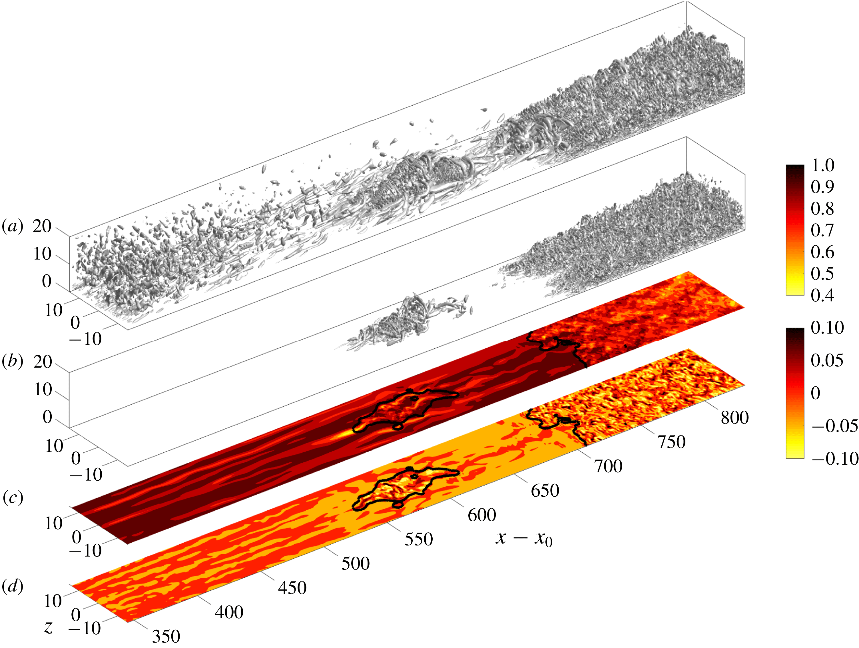
Figure 1. Visualization of a portion of the computational domain for simulations of bypass transition beneath free-stream turbulence with $Tu_{0}=2.5\,\%$ . (a) Vortex visualization highlighting decaying free-stream turbulence ( $\unicode[STIX]{x1D6EC}_{2}$ -criterion,  $\unicode[STIX]{x1D6EC}_{2}=-8\times 10^{-5}$ ); (b) vortex visualization of a turbulent spot ( $\unicode[STIX]{x1D6EC}_{2}=-0.004$ ); (c) contours of the streamwise velocity at $y/\unicode[STIX]{x1D6FF}_{0}=2.78$ ; and (d) contours of the wall-normal velocity at $y/\unicode[STIX]{x1D6FF}_{0}=2.78$ . In (c,d), the black contour corresponds to the boundary of the indicator function separating laminar and turbulent flows.

The two datasets of bypass transition examined in this study differ in their free-stream turbulence intensities, and hence in the onset locations and lengths of the transition zones. The set-up of the computations is shown in figure 1, and the numerical approach is discussed in detail by Nolan & Zaki (Reference Nolan and Zaki2013) and is only briefly summarized here. The incompressible Navier–Stokes equations are solved using a control-volume spatial discretization and a fractional-step algorithm (Rosenfeld, Kwak & Vinokur Reference Rosenfeld, Kwak and Vinokur1991). The diffusion term in the equations for the intermediate velocities are discretized in time using Crank–Nicolson and the advection terms are discretized using Adams–Bashforth. The solution to the elliptic pressure equation is used to project the intermediate velocity onto a divergence-free field. This algorithm has been adopted in several previous studies of bypass transition of boundary layers over flat plates (e.g. Nolan & Zaki Reference Nolan and Zaki2013) and airfoil geometry (Zaki et al. Reference Zaki, Wissink, Rodi and Durbin2010).

The computational domain starts downstream of the leading edge of a flat plate. Its streamwise, wall-normal and spanwise directions are denoted $x$ , $y$ and $z$ , respectively. The inflow condition at $x=x_{0}$ is a superposition of the Blasius profile and free-stream homogeneous, isotropic turbulence. The latter is evident immediately downstream of the inlet in the visualization of vortical structures in figure 1. The free-stream speed $U_{0}$ and the inlet boundary-layer 99 % thickness are selected as the reference velocity and length scales. The inlet Reynolds number is $Re\equiv U_{0}\unicode[STIX]{x1D6FF}_{0}/\unicode[STIX]{x1D708}=800$ , where $\unicode[STIX]{x1D708}$ is the kinematic viscosity, and therefore $x_{0}=33.2$ . No slip conditions are applied at the bottom wall, an advection boundary condition is applied at the exit plane and periodicity is enforced in the homogeneous spanwise direction. The boundary condition at the top surface is zero shear stress, and also accounts for the displacement thickness of the bottom-wall boundary layer in order to ensure zero streamwise pressure gradient.

The two inlet free-stream turbulence intensities considered are $Tu_{0}=2.5\,\%$ and 3.0 % (see figure 2). Their energy satisfies the von Kármán spectrum,

(2.1) $$\begin{eqnarray}E(\unicode[STIX]{x1D705})=Tu_{0}^{2}\frac{1.196(\unicode[STIX]{x1D705}L_{11})^{4}}{[0.558+(\unicode[STIX]{x1D705}L_{11})^{2}]^{17/6}}L_{11},\end{eqnarray}$$

where $\unicode[STIX]{x1D705}$ is the magnitude of the wavenumber vector and $L_{11}$ sets the wavenumber of the peak $E(\unicode[STIX]{x1D705})$ and was set equal to unity. The spectrum is proportional to $\unicode[STIX]{x1D705}^{4}$ at low wavenumbers and to $\unicode[STIX]{x1D705}^{-5/3}$ in the inertial range, and is similar to that adopted in earlier simulations of bypass transition (e.g. Jacobs & Durbin Reference Jacobs and Durbin2001; Brandt, Schlatter & Henningson Reference Brandt, Schlatter and Henningson2004). The integral length scale normalized by the inlet boundary-layer thickness was $L_{k}/\unicode[STIX]{x1D6FF}_{0}=2$ for both levels of free-stream turbulence.

The focus of the present study is on the late stages of transition, where the turbulence spots have formed and reached a mature size. As a result, the free-stream turbulence has decayed to inappreciable levels by the downstream locations of interest. Two domain lengths are considered, $L_{x}=1200$ and 900, for the low and high turbulence intensities respectively. These streamwise extents ensure that transition to a fully turbulent boundary layer is complete within the computational domain. The domain height $L_{y}$ is at least 40 inlet boundary-layer thicknesses and its width is $L_{z}=30$ (see table 1).

The grid spacing is uniform in the streamwise and spanwise directions. In the wall-normal direction, the grid points were clustered close to the wall using a hyperbolic tangent function. The grid resolution is similar to that adopted by Jacobs & Durbin (Reference Jacobs and Durbin2001), who performed a detailed grid refinement study. Relevant parameters from the simulations, including the simulation time step $\unicode[STIX]{x1D6FF}t$ , are summarized in table 1.

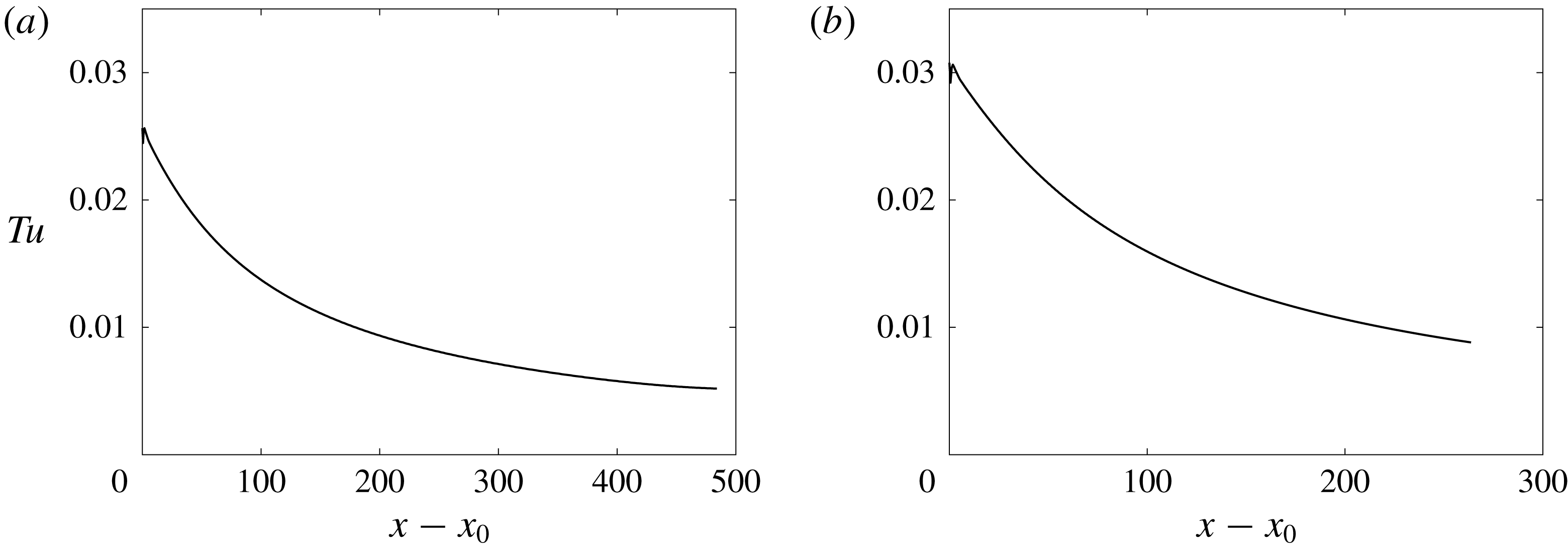
Figure 2. Turbulence level in the free stream as a function of distance from the inflow location $x-x_{0}$ for (a) $Tu_{0}=2.5\,\%$ and (b) $Tu_{0}=3\,\%$ up to the location of transition onset and the intermittency in the boundary layer reaching 10 %.

Table 1. Overview of simulation cases.

For both levels of $Tu_{0}$ , bypass transition takes place: the broadband free-stream turbulence induces streamwise streaks in the boundary layer (see figure 1 c), followed by secondary instability, and ultimately breakdown into turbulence spots; the spots then merge with one another and with the fully turbulent boundary layer downstream. Due to a much longer streamwise and temporal survival of spots at the lower free-stream turbulence intensity, this case enables consideration of spots with a much larger size, yielding higher statistical sampling. A database of instantaneous flow fields from each simulation was used. In the higher $Tu_{0}$ case, the number of fields was $N_{t}=4150$ separated by $\unicode[STIX]{x0394}t=2$ time units, and thus spanning a total period $\unicode[STIX]{x0394}T=8298$ time units. These values are identical to the data used by Nolan & Zaki (Reference Nolan and Zaki2013). The sampling rate was reduced and the duration was extended at the lower $Tu_{0}$ in order to capture sufficient number of turbulence spots. The number of fields was $N_{t}=4560$ separated by $\unicode[STIX]{x0394}t=10$ time units, thus spanning a total period $\unicode[STIX]{x0394}T=45\,590$ time units.

Figure 3. Skin-friction coefficients $C_{f}$ versus downstream distance from the inflow plane $x-x_{0}$ for (a) $Tu_{0}=2.5\,\%$ and (b) $Tu_{0}=3\,\%$ . (——) Standard spanwise- and time-average, (– – –) laminar-conditioned and (— ⋅ —) turbulent-conditioned curves. Grey lines correspond to the skin-friction coefficients for Blasius ( $C_{f}=0.664\,Re_{x}^{-0.5}$ ) and turbulent ( $C_{f}=0.455/\ln ^{2}(0.06Re_{x})$ ) boundary layers. In (c), the results for $Tu_{0}=3\,\%$ are plotted versus momentum-thickness Reynolds number $Re_{\unicode[STIX]{x1D703}}$ , and symbols (○) are a reproduction of the data from figure 8 by Wu & Moin (Reference Wu and Moin2009).

Figure 3 shows the mean skin-friction coefficient, $C_{f}\equiv (\unicode[STIX]{x1D707}\text{d}\overline{u}/\text{d}y)_{y=0}/(0.5\unicode[STIX]{x1D70C}U_{\infty }^{2})$ , where $\unicode[STIX]{x1D707}$ is the dynamic viscosity and overline denotes standard averaging in the homogeneous spanwise direction and in time. The minimum in $C_{f}$ has previously been used to mark the onset of transition, and the downstream maximum to mark the end of the transition zone. Prior to transition, the skin friction is slightly higher than the Blasius value due to the distortion of the base flow by Klebanoff streaks. At the lower free-stream turbulence level, the start of transition is delayed and its length is extended in the streamwise direction. The figure also shows that the case with $Tu_{0}=3\,\%$ possesses a similar transition zone as the simulation by Wu & Moin (Reference Wu and Moin2009). Due to the differences in the free-stream condition, the comparison is not intended to be quantitative; it serves to provide the context for comparing some of our findings to Park et al. (Reference Park, Wallace, Wu and Moin2012) who used data from that study.

Figure 4. Momentum-thickness Reynolds number versus downstream distance from the start of the integration domain $x-x_{0}$ for (a) $Tu_{0}=2.5\,\%$ and (b) $Tu_{0}=3\,\%$ . (——) Standard average, (– – –) laminar-conditioned and (— ⋅ —) turbulent-conditioned curves. Results for a Blasius boundary layer ( $Re_{\unicode[STIX]{x1D703}}=0.664\,Re_{x}^{0.5}$ ) are given for reference (grey).

The downstream dependence of the momentum-thickness Reynolds number, $Re_{\unicode[STIX]{x1D703}}\equiv U_{\infty }\unicode[STIX]{x1D703}/\unicode[STIX]{x1D708}$ is shown in figure 4. While the lengths of the two simulation domains differ, the momentum thicknesses, and as a result the associated $Re_{\unicode[STIX]{x1D703}}$ , reach nearly the same values by the exit planes.

2.2 Data processing procedures

2.2.1 Laminar–turbulent discrimination

In order to compute conditional and ensemble averages of turbulence spots, it is necessary to identify and isolate these turbulent patches from the surrounding non-turbulent flow. Spatial turbulent/non-turbulent discrimination techniques that utilize enstrophy have been applied to flows where turbulence is surrounded by laminar, irrotational flow (Borrell & Jimenez Reference Borrell and Jimenez2016; Lee, Sung & Zaki Reference Lee, Sung and Zaki2017). In the present context, however, the flow outside the turbulence spots is distorted by Klebanoff streaks and, as a result, enstrophy is appreciable in the non-turbulent region. Nolan & Zaki (Reference Nolan and Zaki2013) proposed a laminar–turbulence discrimination algorithm for bypass transition, which we adapt and extend. A detector function is defined using the wall-normal and spanwise velocities, $D\equiv |v|+|w|$ , and a three-dimensional standard deviation filter is applied to $D$ . This filter replaces the local value by the standard deviation of the original data within a surrounding stencil comprised of three points in each coordinate direction. The resulting field is then thresholded in order to generate a binary indicator that is unity in the turbulent region and zero in the non-turbulent zone. This step is performed using Otsu’s method, which identifies the optimum threshold that maximizes the variance between the turbulent and non-turbulent regions, or the inter-class variance.

The procedure is dynamic and the threshold is optimally adjusted for each wall-normal height. The final outcome is a binary indicator function $\unicode[STIX]{x1D6E4}(x,y,z)=\{1,0\}$ , which marks the turbulent and non-turbulent regions, respectively. As an example, the black contour in figure 1(c,d) visualizes the boundary between $\unicode[STIX]{x1D6E4}=1$ inside the turbulent spot and in the fully turbulent boundary layer and $\unicode[STIX]{x1D6E4}=0$ in the non-turbulent flow.

The mean intermittency can be computed using the spanwise and snapshot (or time) average of $\unicode[STIX]{x1D6E4}$ ,

(2.2) $$\begin{eqnarray}\unicode[STIX]{x1D6FE}(x,y)=\frac{1}{\unicode[STIX]{x0394}TL_{z}}\int _{0}^{L_{z}}\int _{t_{0}}^{t_{0}+\unicode[STIX]{x0394}T}\unicode[STIX]{x1D6E4}\,\text{d}t\,\text{d}z,\end{eqnarray}$$

where $\unicode[STIX]{x0394}T$ is the total integration time. In order to characterize the state of the boundary layer as a function of streamwise distance, the maximum intermittency in the wall-normal direction is evaluated,

(2.3) $$\begin{eqnarray}\unicode[STIX]{x1D6FE}_{max}(x)=\max _{y}(\unicode[STIX]{x1D6FE}).\end{eqnarray}$$

This quantity is plotted in figure 5 for both simulations. The results reinforce the observations based on the mean skin-friction coefficient that transition is delayed and prolonged at the lower free-stream turbulent intensity. The intermittency distribution agrees well with a ‘universal’ distribution by Narasimha (Reference Narasimha1957, Reference Narasimha1985), marked by the grey thick line in the figure.

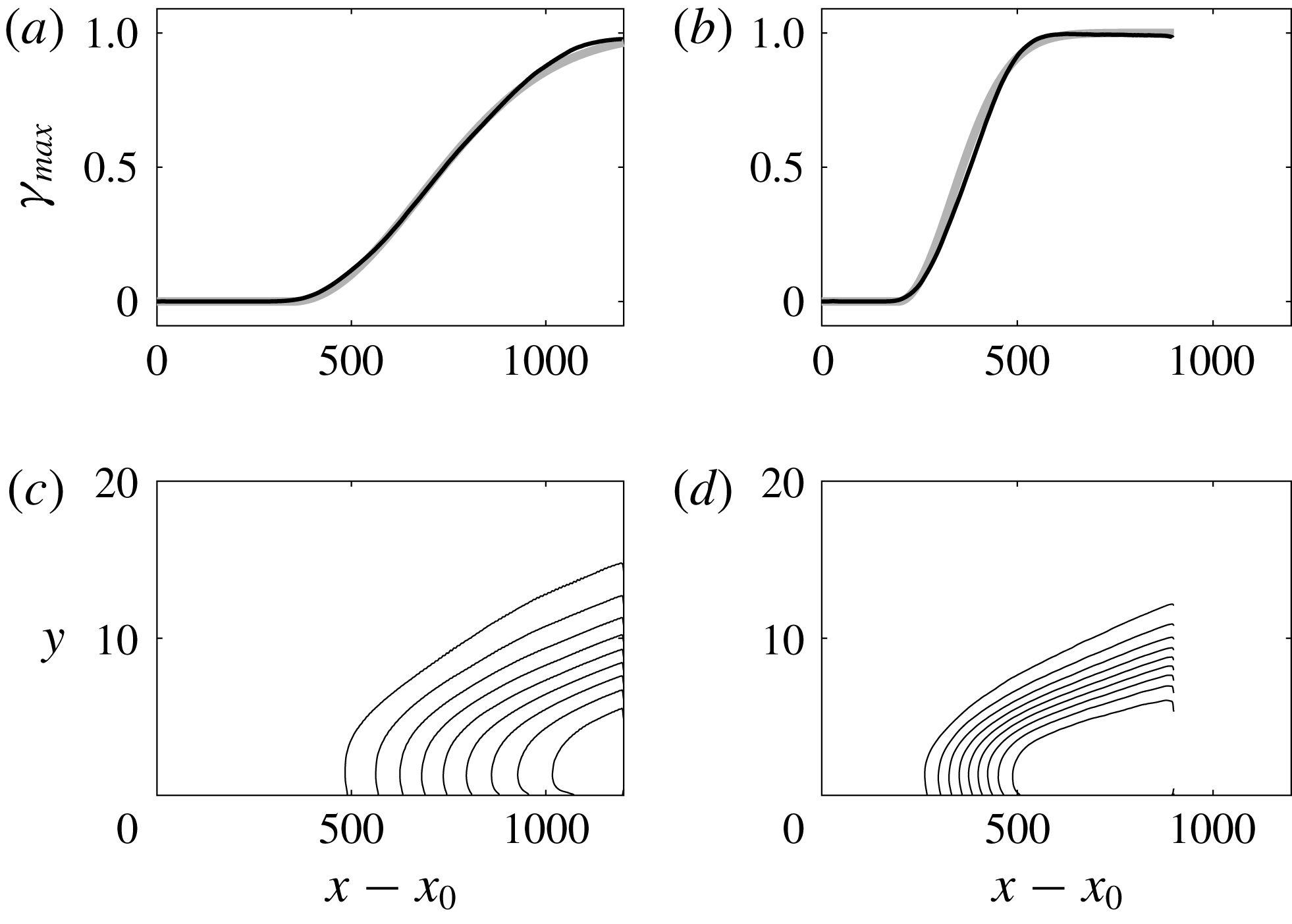
Figure 5. (a,b) Peak intermittency $\unicode[STIX]{x1D6FE}_{max}(x)$ from DNS versus downstream distance from the start of the simulation domain $x-x_{0}$ for (a) $Tu_{0}=2.5\,\%$ and (b) $Tu_{0}=3\,\%$ . The thick grey lines correspond to the relation $\unicode[STIX]{x1D6FE}=1-\exp \left(-0.412\unicode[STIX]{x1D709}^{2}\right)$ where $\unicode[STIX]{x1D709}\equiv \left(x-x_{s}\right)/\left(x_{\unicode[STIX]{x1D6FE}=0.75}-x_{\unicode[STIX]{x1D6FE}=0.25}\right)$ and $x_{s}$ is the onset location of transition (equation (4.8) in Narasimha Reference Narasimha1985). (c,d) Contours of intermittency $0.1\leqslant \unicode[STIX]{x1D6FE}(x,y)\leqslant 0.9$ for (c) $Tu_{0}=2.5\,\%$ and (d) $Tu_{0}=3\,\%$ .

Two statistical approaches are applied to the laminar–turbulence discriminated flow fields in the transition zone: conditional and ensemble averaging. The corresponding procedures are described in §§ 2.2.2 and 2.2.3. For conditional averaging, the flow field is viewed as a juxtaposition of laminar and turbulent states in space and time. At each spatial location and time instance, the flow is classified as laminar or turbulent and statistics of the corresponding system are updated with the new samples. In the transition region, as turbulence spots advect past the point of interest, they each contribute to the conditional average. The turbulent-conditioned statistics can be compared to those from fully turbulent boundary layers at similar conditional Reynolds numbers. In this approach, statistical convergence of turbulent-conditioned data is relatively easier to achieve at higher intermittencies, and gradients of these statistics can be evaluated accurately. Near the start of transition, however, the intermittency is low ( $\unicode[STIX]{x1D6FE}_{max}(x)<0.1$ ), and the number of turbulent samples becomes very small. Therefore, in some figures data involving gradients are omitted for $\unicode[STIX]{x1D6FE}_{max}(x)<0.1$ . The same issue arises in the wall-normal direction towards the free-stream edge of the boundary layer, where the wall turbulence decays and gives way to the free stream; there too $\unicode[STIX]{x1D6FE}$ decays to zero. As a result, absent a prohibitively long time series, turbulent-conditioned averages become unreliable in those regions. In addition, simple conditional averaging does not distinguish the contribution from spots of various sizes: large spots can be expected to have developed turbulence in their core, and to have a relatively small region near their boundaries where the turbulence relaxes to the external non-turbulent state; the turbulence within younger spots, on the other hand, might be less developed and the edge effects could be more pronounced.

The above observations, and the statistically non-stationary nature of turbulence spots, motivate use of ensemble averaging. This approach requires a reasonable number of realizations, or spots, with similar properties to be included in the ensemble Here, it is assumed that the volume of the spot is a good proxy for selecting spots for averaging. Spot inception is sporadic in space and time, and they grow downstream. Therefore, the number of spots that share the same volume at a given streamwise location is limited. Since the change in Reynolds number across the transition zone is gradual, spots were selected for averaging based on their volume and we allowed a shift in the streamwise direction to align their centres of mass. A similar shift was performed in the spanwise direction without any additional assumptions due to homogeneity in that dimension.

2.2.2 Unconditional and conditional statistics

For a general flow quantity, $f$ , conditional averages of turbulent and laminar events are evaluated in the homogeneous spanwise direction and time,

(2.4) $$\begin{eqnarray}\displaystyle & \displaystyle \overline{f}^{(t)}\equiv \frac{1}{\unicode[STIX]{x0394}TL_{z}\unicode[STIX]{x1D6FE}}\int _{0}^{L_{z}}\int _{t_{0}}^{t_{0}+\unicode[STIX]{x0394}T}\unicode[STIX]{x1D6E4}f\,\text{d}t\,\text{d}z, & \displaystyle\end{eqnarray}$$

(2.5) $$\begin{eqnarray}\displaystyle & \displaystyle \overline{f}^{(l)}\equiv \frac{1}{\unicode[STIX]{x0394}TL_{z}(1-\unicode[STIX]{x1D6FE})}\int _{0}^{L_{z}}\int _{t_{0}}^{t_{0}+\unicode[STIX]{x0394}T}(1-\unicode[STIX]{x1D6E4})f\,\text{d}t\,\text{d}z. & \displaystyle\end{eqnarray}$$

Time averaging was performed over the number of snapshots in the database. The conventional average can be reconstructed from the conditional quantities,

(2.6) $$\begin{eqnarray}\overline{f}\equiv \frac{1}{\unicode[STIX]{x0394}TL_{z}}\int _{0}^{L_{z}}\int _{t_{0}}^{t_{0}+\unicode[STIX]{x0394}T}f\,\text{d}t\,\text{d}z=\unicode[STIX]{x1D6FE}\overline{f}^{(t)}+(1-\unicode[STIX]{x1D6FE})\overline{f}^{(l)}.\end{eqnarray}$$

For all the quantities considered in this work, snapshot averages were compared to running averages that were evaluated during the simulations to ensure statistical convergence. From the conditional mean-velocity profiles in the intermittent region, the laminar and turbulent skin-friction coefficients can be evaluated, and are plotted in figure 3. Where the intermittency is zero or unity, the laminar- and turbulent-conditioned $C_{f}$ match the mean. Within the transition zone, the laminar-conditioned curve rises due to the distortion of the flow in calmed regions, which lie in the wake of turbulence spots and of the fully turbulent boundary layer. The turbulent-conditioned $C_{f}$ starts below the turbulent correlation, which is an indication that turbulence spots are not necessarily regions of developed turbulence. The conditionally averaged $Re_{\unicode[STIX]{x1D703}}$ is plotted in figure 4. Note that the definition of the momentum thickness $\unicode[STIX]{x1D703}$ is sensitive to the differences between the conventional mean-velocity profile, which is uniform in the free stream, and the turbulent-conditioned mean profile, which is zero outside the boundary layer. Nonetheless, the turbulent-conditioned $Re_{\unicode[STIX]{x1D703}}$ curves provide a measure of the local Reynolds number to enable comparison of the conditional statistics in the transition zone to fully turbulent boundary layers.

Perturbations can be evaluated relative to either the unconditional or conditional mean, and therefore different symbols are generally needed to reflect the particular choice. However, since in the present work we only report statistics of the perturbations, only a prime is used, and the designation of the average identifies the choice of the mean. For example, the variances of the perturbations relative to the total, turbulent and laminar means are

(2.7a-c ) $$\begin{eqnarray}\displaystyle \overline{f^{\prime 2}}=\overline{f^{2}}-\overline{f}^{2},\quad \overline{f^{\prime 2}}^{(t)}=\overline{f^{2}}^{(t)}-{\overline{f}^{(t)}}^{2},\quad \overline{f^{\prime 2}}^{(l)}=\overline{f^{2}}^{(l)}-{\overline{f}^{(l)}}^{2}. & & \displaystyle\end{eqnarray}$$

Similar to the mean, the variance can be reconstructed from the conditional quantities,

(2.8) $$\begin{eqnarray}\overline{f^{\prime 2}}=\unicode[STIX]{x1D6FE}\overline{f^{\prime 2}}^{(t)}+(1-\unicode[STIX]{x1D6FE})\overline{f^{\prime 2}}^{(l)}+\unicode[STIX]{x1D6FE}(1-\unicode[STIX]{x1D6FE})(\,\overline{f}^{(t)}-\overline{f}^{(l)})^{2}.\end{eqnarray}$$

The expression for the Reynolds stress becomes

(2.9) $$\begin{eqnarray}\overline{u_{i}^{\prime }u_{j}^{\prime }}=\unicode[STIX]{x1D6FE}\overline{u_{i}^{\prime }u_{j}^{\prime }}^{(t)}+(1-\unicode[STIX]{x1D6FE})\overline{u_{i}^{\prime }u_{j}^{\prime }}^{(l)}+\unicode[STIX]{x1D6FE}(1-\unicode[STIX]{x1D6FE})(\overline{u_{i}}^{(t)}-\overline{u_{i}}^{(l)})(\overline{u_{j}}^{(t)}-\overline{u_{j}}^{(l)}).\end{eqnarray}$$

Figure 6 shows a comparison between the standard-averaged variances for the streamwise and wall-normal velocity perturbations, and their conditional values at $\unicode[STIX]{x1D6FE}_{max}=0.5$ . A simple average of the two curves is not appropriate because the intermittency depends on the wall-normal coordinate, and the total variance should also account for the difference between the laminar- and turbulent-conditioned means (see (2.9)). The latter effect is appreciable for the streamwise velocity as the mean flow is distorted from a laminar to a turbulent profile.

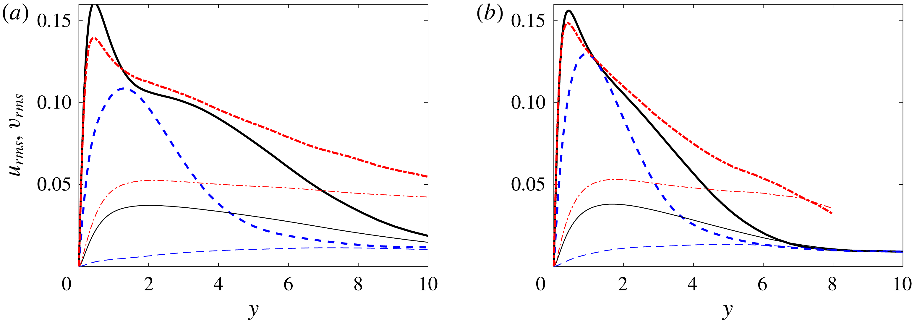
Figure 6. Profiles of the root-mean-square (r.m.s.) streamwise and wall-normal velocity perturbations (thick lines: $u_{rms}$ ; thin lines: $v_{rms}$ ) at the streamwise location where $\unicode[STIX]{x1D6FE}_{max}=0.5$ for (a) $Tu_{0}=2.5\,\%$ and (b) $Tu_{0}=3\,\%$ . (——) Standard spanwise- and time-average, (– – –) laminar-conditioned and (— ⋅ —) turbulent-conditioned curves.

We will also examine terms in the turbulence kinetic energy (TKE) equation,

(2.10) $$\begin{eqnarray}\overline{u_{i}}^{(t)}\frac{\unicode[STIX]{x2202}k^{(t)}}{\unicode[STIX]{x2202}x_{i}}={\mathcal{P}}^{(t)}-\unicode[STIX]{x1D700}^{(t)}+{\mathcal{V}}^{(t)}-\frac{1}{2}{\mathcal{T}}^{(t)}-{\mathcal{R}}^{(t)}.\end{eqnarray}$$

When the superscript $t$ is included, the equation refers to the turbulent-conditioned budget. The unconditional equation can be recovered from an intermittency weighting of the laminar- and turbulent-conditioned parts plus additional terms due to the difference in the conditional base flows. This relationship is not used in the present work, although we have verified it for all reported statistics. It should also be noted that, unlike the standard mean, the conditional average does not commute with the derivative operator unless derivatives of the intermittency are taken into account. Explicit forms of the terms in (2.10) are given in appendix A.

2.2.3 Detection of turbulence spots and ensemble averaging

The procedure to generate ensemble-averaged data of spots in the transition zone consists of two steps: identification of inception locations of spots and their tracking in space and time; and the selection of the ensemble members for averaging. These steps are described in the following.

In the present study, an instance of the turbulent spot is identified as a connected region of turbulence, surrounded by non-turbulent flow. Some small patches of disturbed flow may form in the transition region and subsequently decay without maturing into turbulence spots. The lifetime of these evanescent regions is less than $\unicode[STIX]{x1D6FF}/U_{\infty }$ , and as such they only appear in a single snapshot and are discarded.

The location and time of spot inception are evaluated using $\unicode[STIX]{x1D6E4}(x,y,z,t)$ . A four-dimensional array is formed, which contains the three-dimensional and time-dependent binary indicator function. This array is examined using a translating time window, which considers three consecutive snapshots. Connected components are identified, and regions with $\unicode[STIX]{x1D6E4}=1$ throughout the three time instances are classified as an established spot. If the connectivity spans only the last two instances, the region is labelled an emerging spot, and its volume  and inception location and time ( $x_{s,i}$ and $T_{s,i}$ ) are tabulated. Components that are present only in a single snapshot are discarded. After this procedure, a table with all spot inception times and locations is available, and is used for spot tracking.

Using the four-dimensional connected objects to track spots is not viable due to spot merging events that occur regularly. Instead, the tracking algorithm relies on the advection velocity and spreading rate of the turbulence patches, which are initialized and corrected using actual data. Starting from the spot inception location and time, the advection velocity is used to estimate an anticipated downstream location at a later time, and the spreading rate sets a spatial search window. If the spot crosses the edges of the spatial window, the window is enlarged in order to encompass the entire turbulent patch. Failure to enclose the patch indicates that it has either merged with itself across the span or with the downstream fully turbulent region; in this case, the tracking is terminated. For every tracked spot, both the location of its centre of volume, , and its volume, , are calculated and this information is saved as a function of time since inception. When discussing the spatial structure of turbulence spots, we will adopt the following convention: locations with $x$ -coordinate downstream of the centre of volume of the spot    will be referred to as the front, whereas the rear of the spot refers to points with . Spots with similar volume are selected for averaging. Specifically, the spot volume must lie within a certain range . The volume of a spot corresponds to the sum of all cell volumes for which the indicator function $\unicode[STIX]{x1D6E4}=1$ . The table generated during spot tracking is searched, and every spot that satisfies this bound during its evolution is selected for sampling. When multiple snapshots during a spot history satisfy the criterion, the instance when the volume is closest to the mid-point of the range is selected. The spots are subsequently shifted in the spanwise and streamwise directions in order to align their centres.

The volume range in the present study is $[7600,14\,000]$ , and more than 50 spots from each simulation fulfil this criterion. The number of samples is further increased by exploiting the spanwise symmetry of the flow, which enables sampling of the spanwise mirror images of the patches. Although the sample size is not very large, it is sufficient to highlight the global features of turbulence within the spots.

Two different ensemble averages are performed, and will be referred to as (i) the unconditional and (ii) the turbulent ensembles. The first approach shifts the entire flow field in the streamwise and spanwise directions in order to align the centres of the spots. The ensemble average is then performed using the entire flow field. The advantages of this method are that all spatial points within and surrounding the spots have the same sample size and that derivatives in all spatial directions can be readily evaluated, which facilitates computing all terms in the turbulence kinetic energy equation. A two-dimensional spatial filter in the horizontal plane with size $(4\unicode[STIX]{x0394}x,4\unicode[STIX]{x0394}z)$ was also applied in order to regularize the computation of derivatives. The main disadvantages of the unconditional ensemble is that the spot shape is not evident from this procedure. Therefore, results are supplemented with an outline of the ensemble spot shape (see e.g. figure 18). In addition, both laminar and turbulent regions contribute to the ensemble average near the edges of the turbulence spots, because the patches vary in shape. The second approach only considers turbulent-conditioned data. In this case, only turbulent signals contribute to the ensemble average near the edges of the spots. Due to the variability in spot geometry, the sample size reduces towards the spot boundaries and spatial derivatives cannot be easily computed.

The paths and volumes of all the spots from the database with inflow $Tu=2.5\,\%$ are shown in figure 7. Sudden changes in volume and position mark merging events. The figure also shows the maximum intermittency factor $\unicode[STIX]{x1D6FE}_{max}$ , with circles that mark $\unicode[STIX]{x1D6FE}_{max}=0.1$ , 0.25 and 0.5. The spot centres are seldom observed beyond the streamwise location where $\unicode[STIX]{x1D6FE}_{max}=0.5$ , as the spots reach a sufficiently large size and either merge in the span or with the downstream fully turbulent boundary layer.

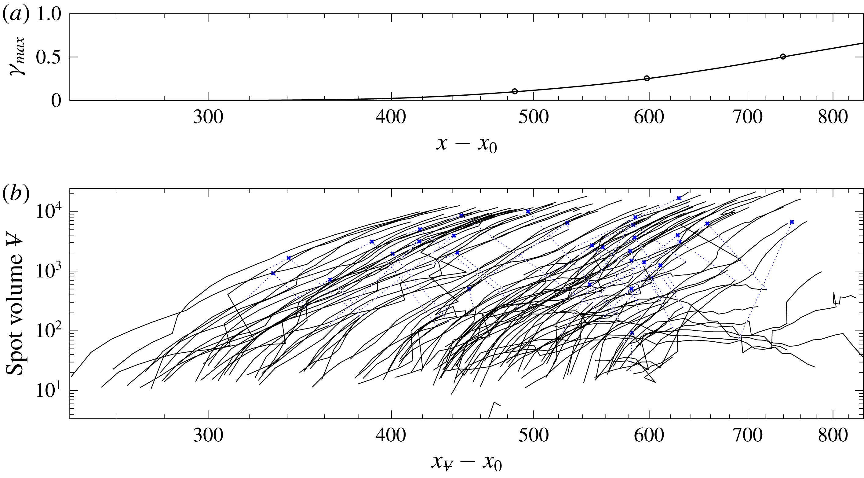
Figure 7. (a) Maximum intermittency $\unicode[STIX]{x1D6FE}_{max}$ and (b) spot volume as a function of streamwise distance, for $Tu_{0}=2.5\,\%$ . The circles in (a) mark $\unicode[STIX]{x1D6FE}_{max}=0.1$ , 0.25 and 0.5. The blue crosses in (b) label locations of spot merging, and the dotted lines connect the two paths of spots that undergo merging.

The range of spot inception locations is substantially reduced for the larger inflow turbulence level (not shown), and the slope of the maximum intermittency curve is steeper. Similar to the lower $Tu$ , however, spot tracking remains effective only upstream of $\unicode[STIX]{x1D6FE}_{max}\approx 0.5$ , beyond which the spots merge with the irregular edge of the downstream turbulent boundary layer.

3.1 Standard and turbulent-conditioned data in the fully turbulent region

Prior to examining the flow in the transition zone, we present conventional and turbulent-conditioned statistics in the region where the turbulence intermittency is above 90 % and the boundary layer is nearly fully turbulent. The results are also compared to data from the simulations by Spalart (Reference Spalart1988).

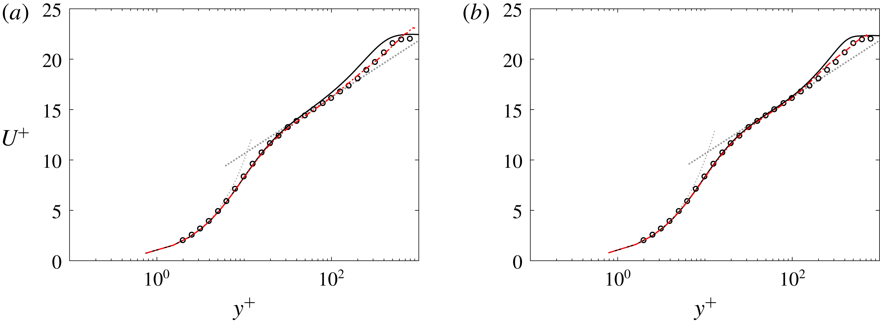
Figure 8. Mean-flow profiles of the streamwise velocity in wall units at the streamwise location $x$ where (a) $Re_{\unicode[STIX]{x1D703}}=1223$ , $Tu_{0}=2.5\,\%$ and (b) $Re_{\unicode[STIX]{x1D703}}=1226$ , $Tu_{0}=3\,\%$ . Standard-averaged (——) and turbulent-conditioned quantities (— ⋅ —) are plotted. The dotted lines correspond to the law of the wall $u^{+}=y^{+}$ and the log law $u^{+}=1/0.41\log y^{+}+5$ . Symbols are data for a turbulent boundary layer at $Re_{\unicode[STIX]{x1D703}}=1410$ from figure 24 by Spalart (Reference Spalart1988).

Figure 8 shows the conventionally and turbulent-conditioned mean streamwise velocity profiles. In order to provide data at the same momentum-thickness Reynolds numbers, $Re_{\unicode[STIX]{x1D703}}\approx 1225$ , the intermittency deviates slightly among the two computations with $\unicode[STIX]{x1D6FE}_{max}\approx \{0.95,0.99\}$ for $Tu_{0}=\{2.5,3.0\}\,\%$ . The data from Spalart (Reference Spalart1988) at $Re_{\unicode[STIX]{x1D703}}=1410$ are also included in the figure. The results establish that the downstream boundary layer in the present simulations approaches the fully turbulent state. The turbulent-conditioned profiles match the conventional mean in the viscous sublayer and through the log layer. The deviation between the conventional and conditional averages appears in the wake region, near the edge of the boundary layer, because turbulence intermittency decays towards zero in the free stream (Lee & Zaki Reference Lee and Zaki2017).

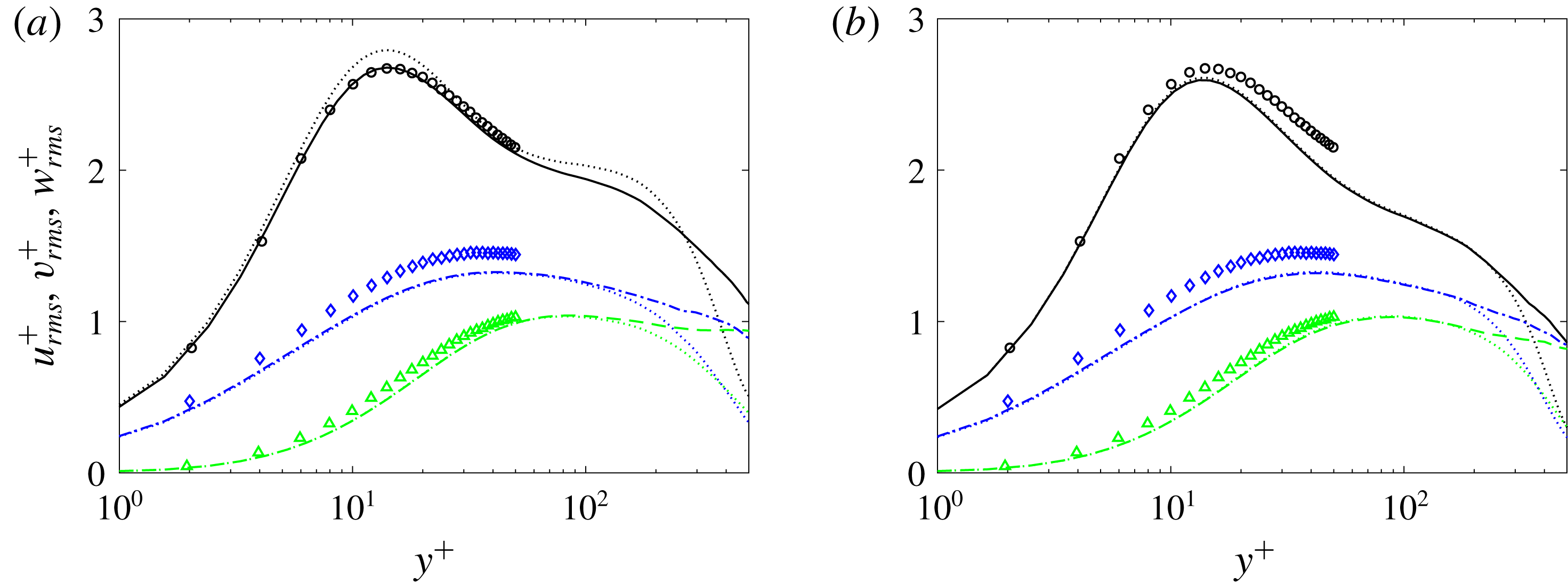
Figure 9. Conditionally averaged turbulent intensities ( $u^{+},w^{+},v^{+}$ from top to bottom) in plus coordinates at the streamwise location $x$ where (a) $Re_{\unicode[STIX]{x1D703}}=1223$ , $Tu_{0}=2.5\,\%$ and (b) $Re_{\unicode[STIX]{x1D703}}=1226$ , $Tu_{0}=3\,\%$ . Conventionally averaged quantities are given as dotted lines. Symbols are data for a turbulent boundary layer at $Re_{\unicode[STIX]{x1D703}}=1410$ from figure 13 by Spalart (Reference Spalart1988).

Profiles of the Reynolds normal stresses are plotted in figure 9 for the same streamwise positions as in figure 8. In the region $y^{+}\lesssim 200$ , the conventional and turbulent-conditioned data show good agreement for the higher $Tu$ case, because the intermittency is near unity at the shown location. For the lower $Tu$ case, the two averages deviate because the intermittency at that streamwise position is 95 %. In both cases, as the intermittency decays near the edge of the boundary layer, the two curves deviate with the turbulent-conditioned curves decaying less quickly than the conventional profiles. The latter are contaminated by contributions from the differences between the conditional means, or the term $(\overline{u}^{(t)}-\overline{u}^{(l)})$ in (2.9).

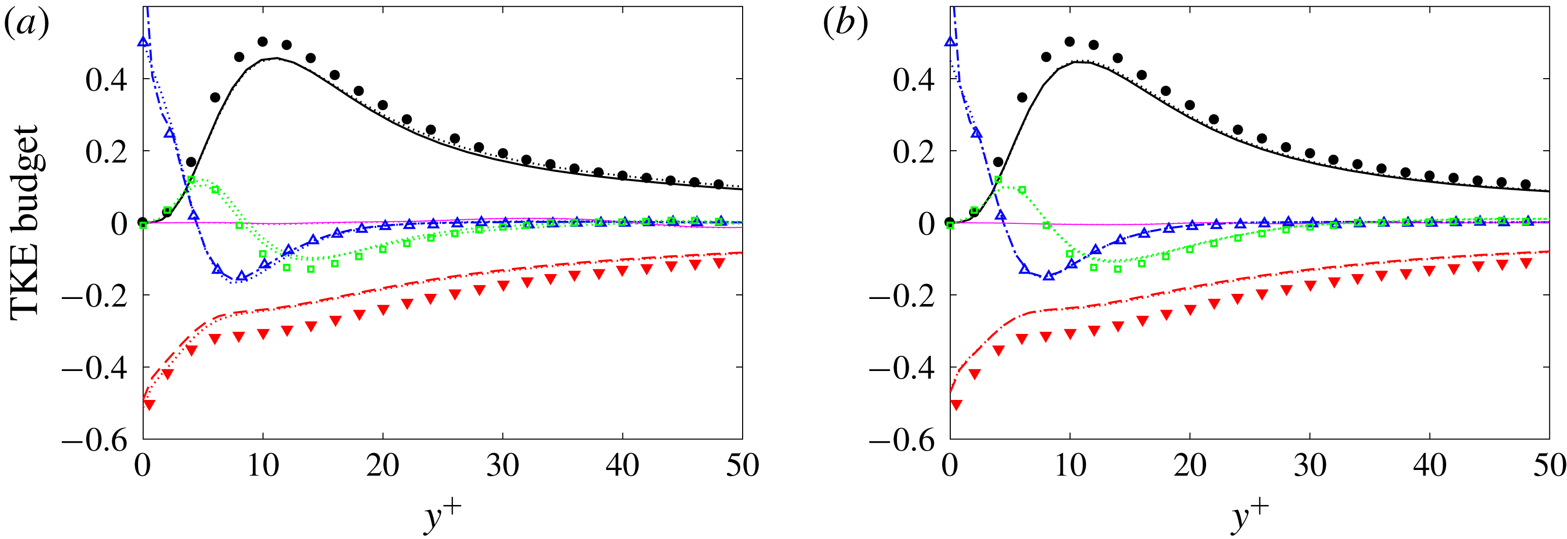
Figure 10. Conditionally averaged TKE budget terms at the streamwise location $x$ where (a) $Re_{\unicode[STIX]{x1D703}}=1223$ , $Tu_{0}=2.5\,\%$ and (b) $Re_{\unicode[STIX]{x1D703}}=1226$ , $Tu_{0}=3\,\%$ . Conventionally averaged quantities are given as dotted lines. Production (——, $\bullet$ ); turbulent convection ( $\cdots \cdots$ , ▫); viscous diffusion (— ⋅ —, ▵); mean advection (——); dissipation (– – –, ▾). Symbols are data for a turbulent boundary layer at $Re_{\unicode[STIX]{x1D703}}=1410$ from figure 24 by Spalart (Reference Spalart1988).

A comparison of the TKE budget terms is shown in figure 10. For both free-stream turbulence intensities, the conventional and turbulent-conditioned statistics are indistinguishable because the figure focuses on the near-wall region. The deviation from the data by Spalart (Reference Spalart1988) is small.

Based on these comparisons, the present simulations of bypass transition lead to a boundary layer that approaches the fully turbulent state that is well documented in the literature. The flow field in the transitional regime will be examined next, with particular focus on the conditional statistics, and how they compare to conventionally averaged quantities.

3.2 Streamwise evolution of turbulent-conditioned data in the transition zone

We begin by considering the downstream evolution of flow quantities as a function of $\unicode[STIX]{x1D6FE}_{max}$ . Figure 11 shows the skin-friction coefficient obtained from conventional and turbulent-conditioned averaging. As anticipated, the values from standard averaging increase monotonically as a function of maximum intermittency $\unicode[STIX]{x1D6FE}_{max}$ , except when $\unicode[STIX]{x1D6FE}_{max}$ nearly vanishes or is unity. On the other hand, the turbulent-conditioned curves only show a weak dependence on $\unicode[STIX]{x1D6FE}_{max}$ for the majority of the range. This is in contrast to monotonically decreasing values of the turbulent skin friction expected with an increase in the local Reynolds number, shown in figure 11 by the empirical correlations (dotted lines).

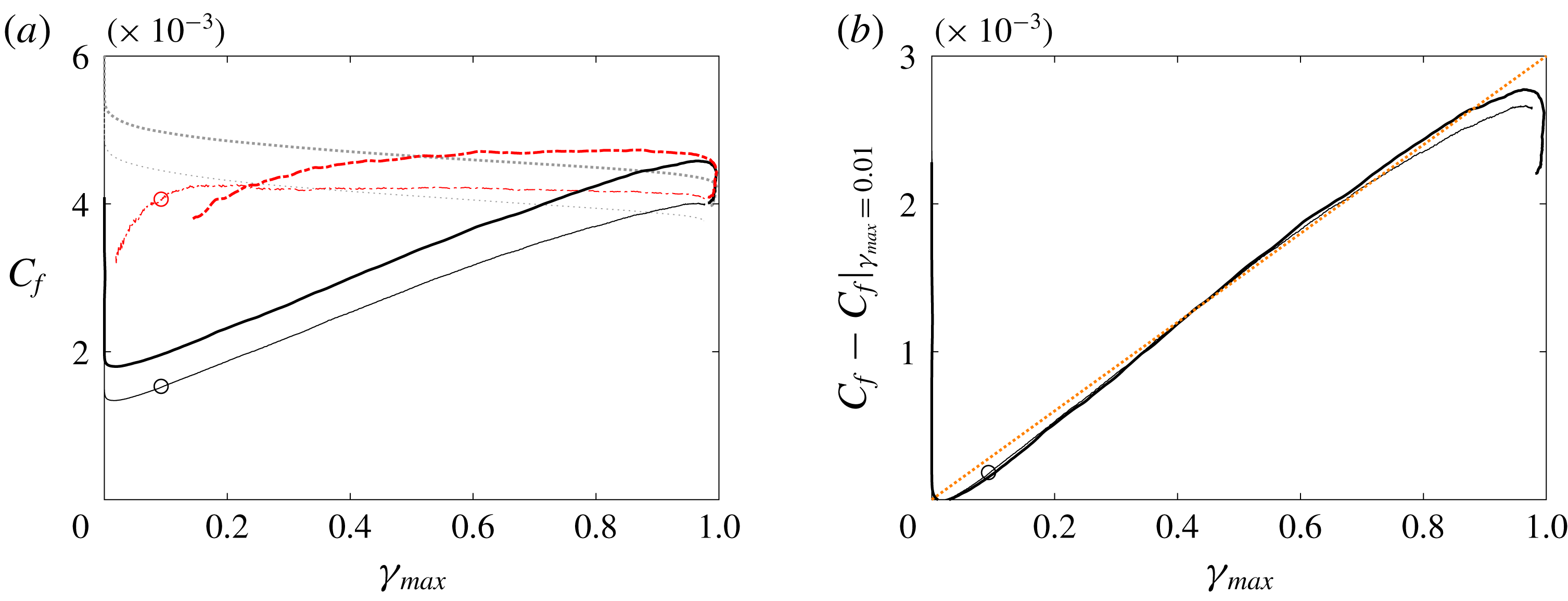
Figure 11. (a) Skin-friction coefficient $C_{f}$ and (b) departure from the laminar value $C_{f}-C_{f}|_{\unicode[STIX]{x1D6FE}_{max}=0.01}$ versus $\unicode[STIX]{x1D6FE}_{max}$ . Standard-averaged ( $Tu_{0}=3\,\%$ : ——; $Tu_{0}=2.5\,\%$ : thin lines with marker ○) and turbulent-conditioned (— ⋅ —) results. (a) The dotted lines ( $\cdots \cdots$ ) correspond to the turbulent correlation ( $C_{f}=0.455/\ln ^{2}(0.06Re_{x})$ . (b) The dotted line marks a linear dependence.

While the turbulent-conditioned skin-friction coefficient appears nearly constant in the transition zone, its contribution to the total value is weighted by the intermittency and hence increases downstream. This cumulative contribution of the turbulence can be highlighted by subtracting the laminar skin-friction coefficient which is recorded at the onset of transition, and plotting $C_{f}-C_{f}|_{\unicode[STIX]{x1D6FE}_{max}=0.01}$ versus $\unicode[STIX]{x1D6FE}_{max}$ (figure 11 b). The results show that the curves from both computations, with low and high free-stream intensities, collapse and become proportional to the intermittency. In light of (2.6), the linear dependence of $C_{f}$ on $\unicode[STIX]{x1D6FE}$ is due to the fact that the laminar-conditioned skin-friction coefficient contributes little to the standard-averaged $C_{f}$ , while at the same time the turbulent-conditioned $C_{f}$ is almost constant in the intermittent region and does not exhibit a decay with increasing downstream location.

The peak values of the r.m.s. perturbations $v^{\prime }$ and $w^{\prime }$ are plotted versus the maximum intermittency in figure 12. The most notable observation is perhaps that the r.m.s. values from the two simulations are very similar, except for the laminar-conditioned data. In the laminar region upstream of the shown range, $v^{\prime }$ and $w^{\prime }$ inside the boundary layer are merely the near-wall signatures of the free-stream turbulence and hence differ (dashed lines in the figure). However, once transition is initiated, $v^{\prime }$ and $w^{\prime }$ perturbations amplify largely due to the redistribution of energy from the pre-transitional streaky $u^{\prime }$ field. As a result, the rate of increase of the conventional r.m.s. value is high in the early transitional zone, but subsequently weakens. The corresponding turbulent-conditioned data show an initial sharp rise at transition onset, within a very narrow region, and decay monotonically for the majority of the range of $\unicode[STIX]{x1D6FE}_{max}$ .

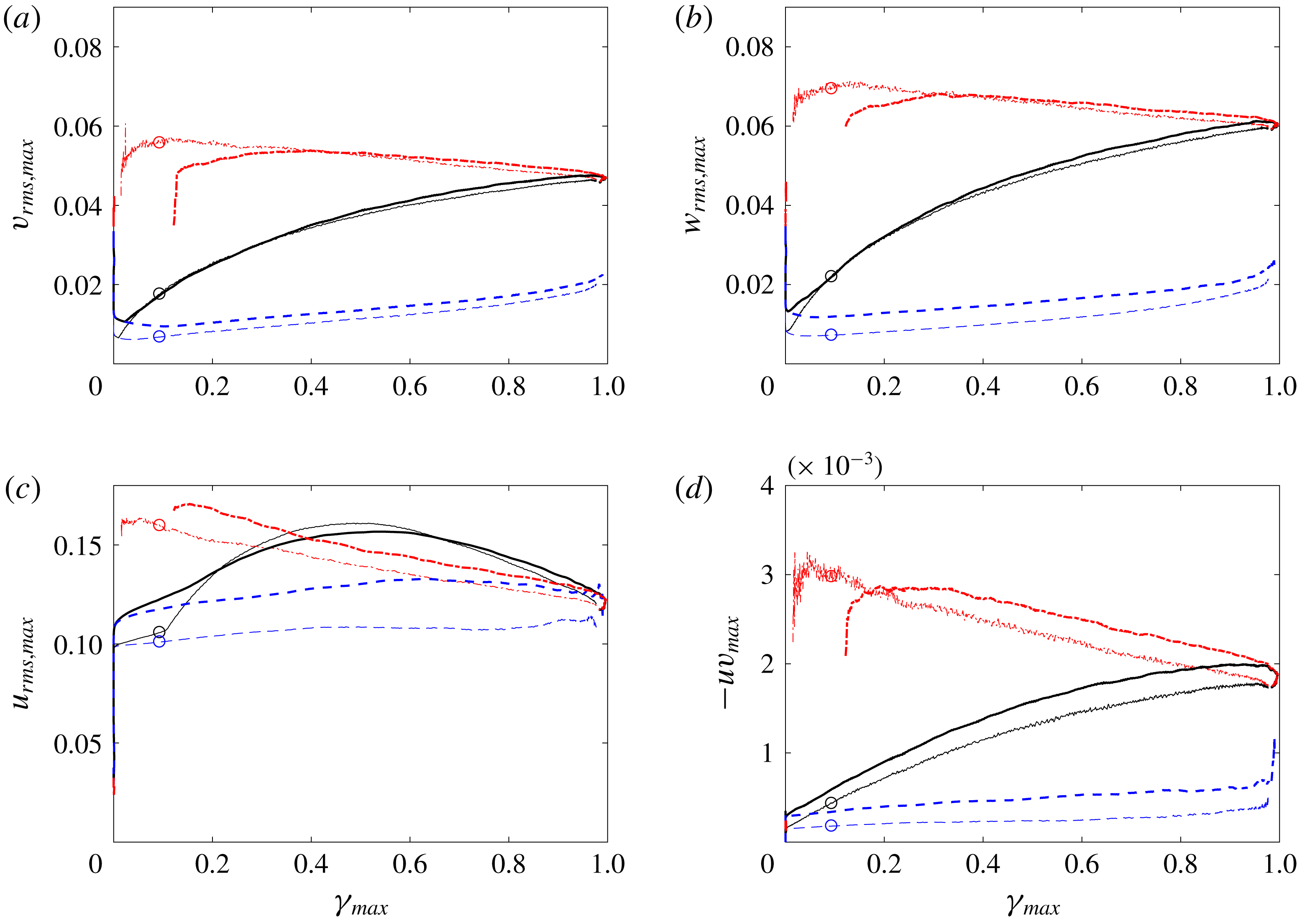
Figure 12. Wall-normal peak values of (a) $v_{rms}$ , (b) $w_{rms}$ , (c) $u_{rms}$ and (d) $-uv_{max}$ versus $\unicode[STIX]{x1D6FE}_{max}$ for $Tu_{0}=3\,\%$ (thick lines) and $Tu_{0}=2.5\,\%$ (thin lines with marker ○). Standard-averaged results (——); laminar-conditioned (– – –); and turbulent-conditioned (— ⋅ —) results.

Peak r.m.s. values of the streamwise velocity perturbation and the Reynolds shear stress are shown in figure 12. The curves from the two free-stream turbulence intensities differ, be that for the laminar- or turbulent-conditioned results and, as a result, the conventional statistics as well. The laminar-conditioned results correspond to the pre-transitional streaks, which are higher in amplitude in the case with stronger free-stream forcing. As transition sets in, the resulting turbulent-conditioned results retain some dependence on the original streaky state, thus showing higher values of $\overline{u^{\prime 2}}^{(t)}$ and $\overline{u^{\prime }v^{\prime }}^{(t)}$ . The conventional-average curve for the streamwise velocity peaks near the location where the intermittency reaches 50 %. There, the peak is larger than both the laminar- and turbulent-averaged values, which is due to the contribution of the change in mean velocity to the total stress (2.9).

3.3 Wall-normal profiles of turbulent-conditioned data in the transition zone

The degree to which turbulent-conditioned statistics agree with data from fully turbulent boundary layers is examined at three levels of intermittency, $\unicode[STIX]{x1D6FE}_{max}=\{0.1,0.25,0.5\}$ . These values correspond to turbulence near the onset of spots, in the early stages of transition and when the laminar and turbulent states are equally likely. Since our interest is in the intermittency due to inception of spots, and not due to the undulation of the free-stream edge of the boundary layer, we will focus on the region $y^{+}<200$ . We will also proceed from the highest intermittency, where agreement with the conventional turbulent boundary-layer data is more likely, to successively lower values of $\unicode[STIX]{x1D6FE}_{max}$ . All quantities are normalized by wall units, using the turbulent-conditioned friction velocity.

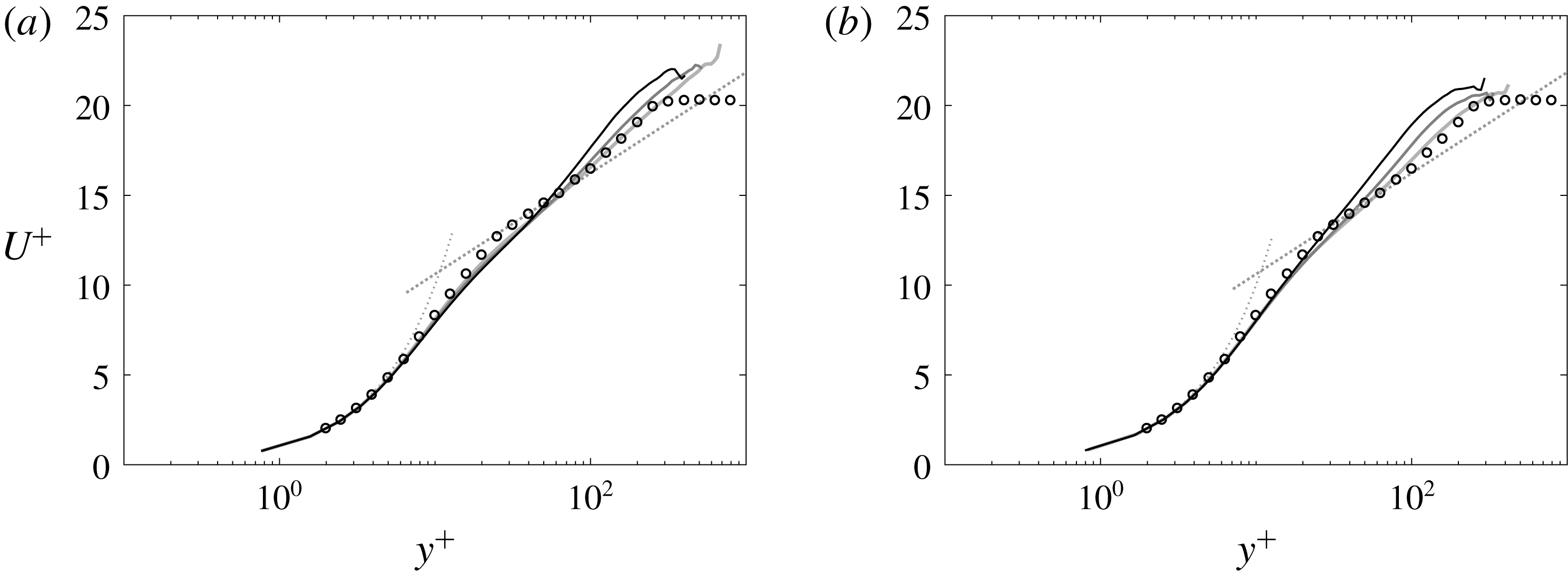
Figure 13. Turbulent-conditioned mean streamwise velocity profile scaled using wall units, and evaluated at the streamwise locations where (dark to light) $\unicode[STIX]{x1D6FE}_{max}=\{0.1,0.25,0.5\}$ . (a) $Tu_{0}=2.5\,\%$ , (dark to light) $Re_{\unicode[STIX]{x1D703},turbulent}=\{731,880,1058\}$ ; (b) $Tu_{0}=3\,\%$ , (dark to light) $Re_{\unicode[STIX]{x1D703},turbulent}=\{566,614,671\}$ . Symbols (○) are data for a turbulent boundary layer at $Re_{\unicode[STIX]{x1D703}}=670$ from Spalart (Reference Spalart1988).

At the three values of $\unicode[STIX]{x1D6FE}_{max}$ , a comparison of the turbulent-conditioned average velocity profiles with the fully developed turbulent-flow data by Spalart (Reference Spalart1988) is shown in figure 13. At 50 % intermittency, the profiles are in very good agreement with the law of the wall, as already highlighted by Nolan & Zaki (Reference Nolan and Zaki2013) (see their figure 11c). The agreement with the data by Spalart (Reference Spalart1988) extends into the buffer layer and also the log layer. Further upstream, at $\unicode[STIX]{x1D6FE}_{max}=0.25$ , the turbulent-conditioned mean profiles start to show deviation from the data away from the wall. The departure near the wake region is affected by the differences in turbulent-conditioned and conventional averages. However, the departure within the log region is due to differences in the turbulent-flow state in that region. When $\unicode[STIX]{x1D6FE}_{max}=0.1$ , the turbulent-conditioned mean profiles are elevated relative to the fully developed turbulent curves. The departure from the log law is pronounced, which suggests that the flow in this early transitional regime is appreciably different from the fully turbulent state.

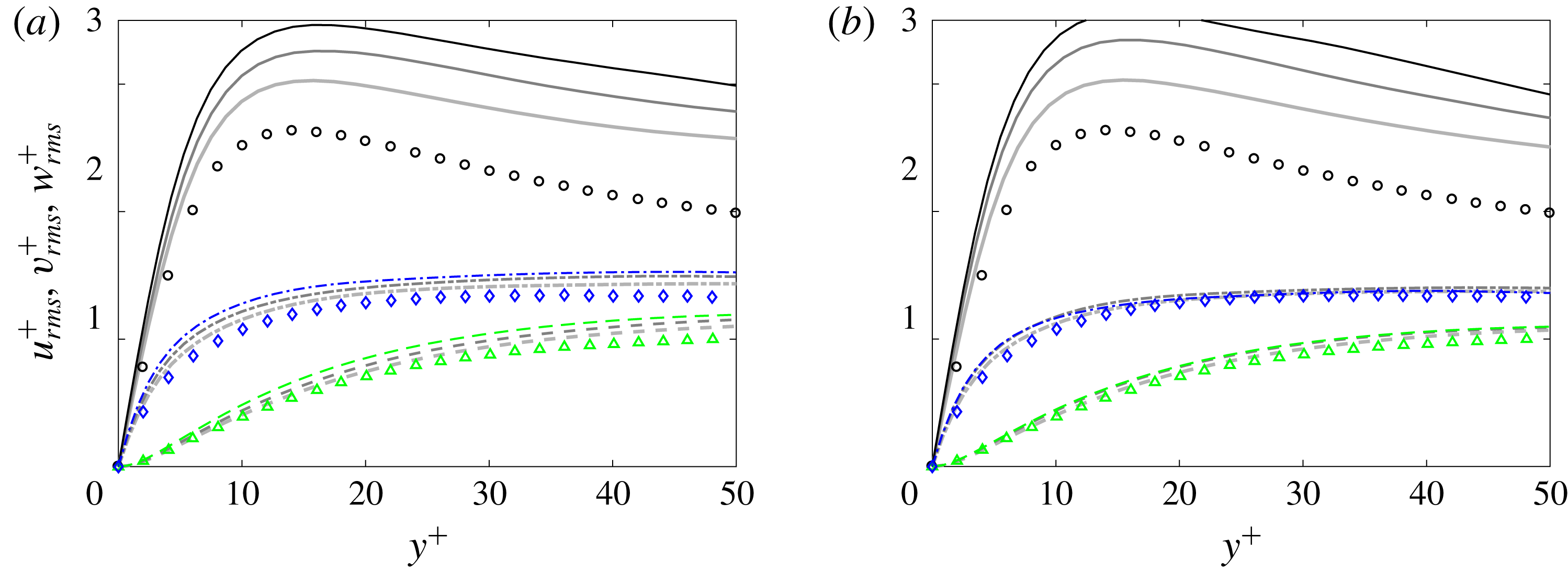
Figure 14. Turbulent-conditioned Reynolds normal stresses scaled using wall units, and evaluated at the streamwise locations where (dark to light) $\unicode[STIX]{x1D6FE}_{max}=\{0.1,0.25,0.5\}$ . (a) $Tu_{0}=2.5\,\%$ , (dark to light) $Re_{\unicode[STIX]{x1D703},turbulent}=\{731,880,1058\}$ ; (b) $Tu_{0}=3\,\%$ , (dark to light) $Re_{\unicode[STIX]{x1D703},turbulent}=\{566,614,671\}$ . Symbols (○) are data for a turbulent boundary layer at $Re_{\unicode[STIX]{x1D703}}=670$ from Spalart (Reference Spalart1988).

Figure 14 displays the turbulent-conditioned r.m.s. profiles normalized by the friction velocity, which are compared to the data by Spalart (Reference Spalart1988). For the wall-normal and spanwise velocity components, excellent agreement is observed throughout the wall-normal range considered at $\unicode[STIX]{x1D6FE}=0.5$ . The agreement only slightly diminishes upstream at lower intermittencies, $\unicode[STIX]{x1D6FE}=0.25$ and 0.1.

Profiles of the turbulent-conditioned streamwise perturbations exhibit higher values than reported for fully turbulent boundary layers, even at $\unicode[STIX]{x1D6FE}=0.5$ . A similar observation was made by Park et al. (Reference Park, Wallace, Wu and Moin2012), although a reason was not proposed. Two potential contributing factors are (i) the influence of the pre-transitional, high-amplitude Klebanoff distortions and (ii) spatial inhomogeneity within turbulence spots. It will be shown in § 4.1 that the two effects are related and, therefore, both contribute to the larger $u_{rms}$ . Upstream of transition, the boundary layer is perturbed by high-amplitude elongated streaks, which undergo secondary instability and lead to the inception of turbulent patches. Their signature does not immediately disappear within the early turbulence within spots, as evident from the surface thermal measurements by Anthony, Jones & LaGraff (Reference Anthony, Jones and LaGraff2005). In addition, the turbulence within the spots must relax to a non-turbulent state beyond the spot perimeter. As a result, the turbulence characteristics near the periphery can deviate from those in equilibrium – a matter further examined using ensemble-averaged data in § 4.

Both effects put forward to explain the deviation in $u_{rms}$ profiles from turbulence data are likely to be more pronounced at lower intermittencies. Near spot inception, the perimeter to area ratio of the turbulence patches is largest and memory of the streaky flow upstream is more pronounced. As a result, larger deviations in the conditionally averaged $u_{rms}$ profiles from the data by Spalart (Reference Spalart1988) are observed at $\unicode[STIX]{x1D6FE}=0.25$ and 0.10. In addition, the deviation is larger for the simulation with higher free-stream turbulence intensity at the earliest upstream location.

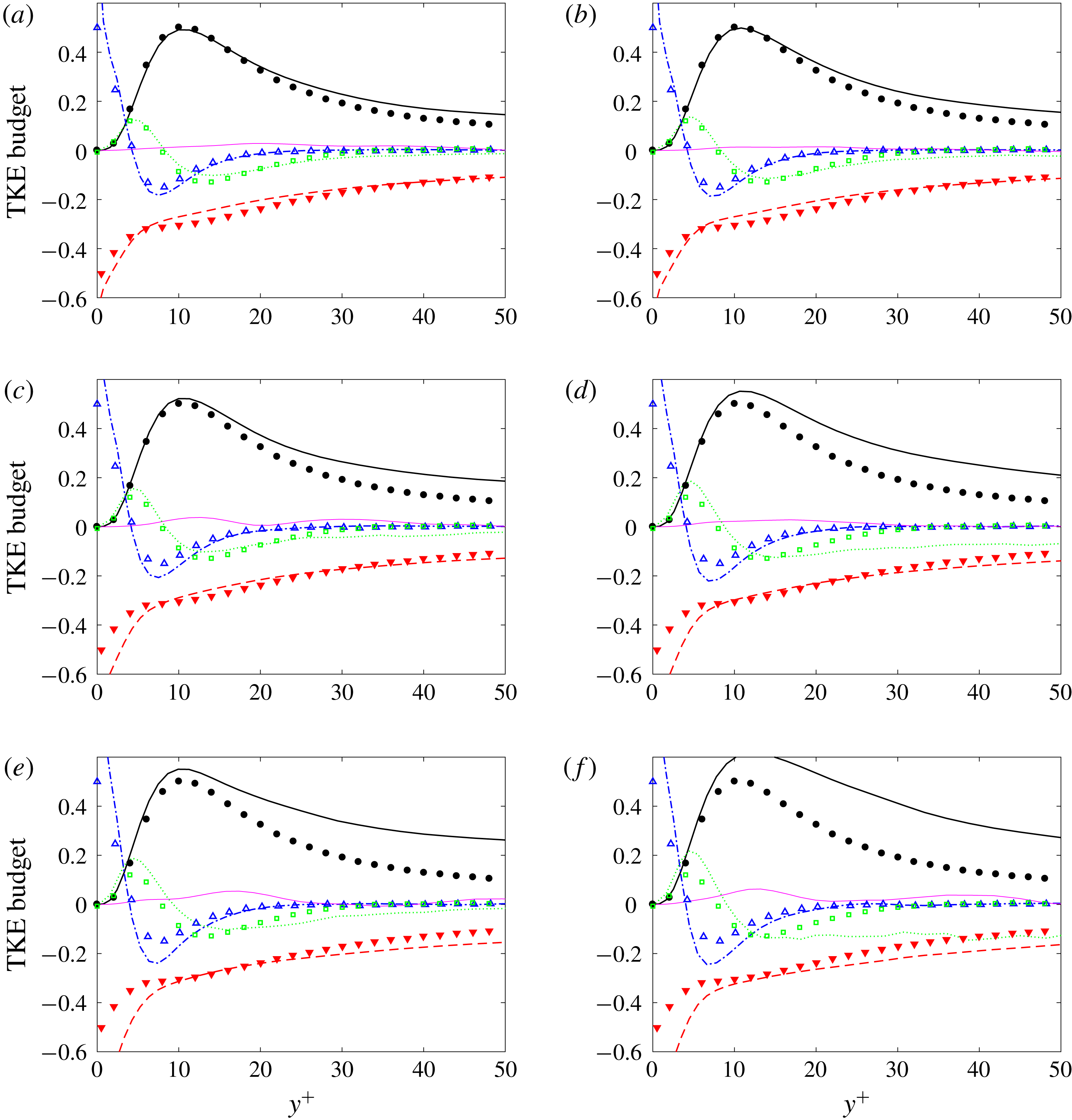
Figure 15. Turbulent-conditioned TKE budget terms at the streamwise location where (a–f) $\unicode[STIX]{x1D6FE}_{max}=\{0.5,0.25,0.1\}$ . (a,c,e) $Tu_{0}=2.5\,\%$ ; (b,d,f) $Tu_{0}=3\,\%$ . Production (——, ●); turbulent convection ( $\cdots \cdots$ , ▫); viscous diffusion (— ⋅ —, ▵); dissipation (– – –, ▾); mean-flow convection (thin solid line). Symbols are data for a turbulent boundary layer at $Re_{\unicode[STIX]{x1D703}}=1410$ from figure 24 by Spalart (Reference Spalart1988).

Terms of the turbulence kinetic energy budget are plotted in figure 15 along with data from Spalart (Reference Spalart1988). At $\unicode[STIX]{x1D6FE}_{max}=0.5$ , good agreement is observed for all terms, although the deviation from the fully turbulent data is more significant than at the higher intermittency stations discussed earlier (see figure 10 for $\unicode[STIX]{x1D6FE}_{max}>0.9$ ). While the turbulence production and dissipation have larger absolute values than the data, the results at $\unicode[STIX]{x1D6FE}_{max}=0.5$ suggest that the turbulence dynamics do not significantly deviate from fully turbulent flows.

The deviation of production from the data starts at $y^{+}>15$ , and becomes more pronounced as the intermittency is reduced to $\unicode[STIX]{x1D6FE}_{max}=0.25$ . It is balanced by more active turbulent transport and diffusion, and ultimately enhanced dissipation at the wall. This trend is further reinforced at lower intermittency, $\unicode[STIX]{x1D6FE}_{max}=0.1$ , with the turbulent-conditioned production appreciably exceeding the data as early as $y^{+}\approx 7$ . The deviation is also more significant when the free-stream $Tu_{0}$ is larger, since the pre-transitional streaks which become sites for the inception of turbulence spots are more energetic. Absolute values of viscous diffusion and dissipation are also much larger at the wall. At this early stage, the profiles of the turbulent-conditioned TKE budget terms start to qualitatively differ from the data, which reinforces the view that the turbulence within the early nascent spots differs from the fully turbulent boundary layer downstream.

The above observations are further supported by examining the behaviour of representative quantities, plotted in wall units, as a function of maximum intermittency (figure 16). All quantities are normalized using the turbulent-conditioned friction velocity. For $\unicode[STIX]{x1D6FE}_{max}\gtrapprox 0.4$ , and hence slightly further into transition than in figure 12, data obtained for the two levels of free-stream $Tu_{0}$ coincide. The collapse indicates that the free-stream perturbation does not have a significant effect on the late stages of transition and early turbulent boundary layer. Upstream, where the flow is not rid of the influence of pre-transitional boundary-layer streaks and therefore $Tu_{0}$ , all shown quantities exhibit a dependence on $\unicode[STIX]{x1D6FE}_{max}$ .

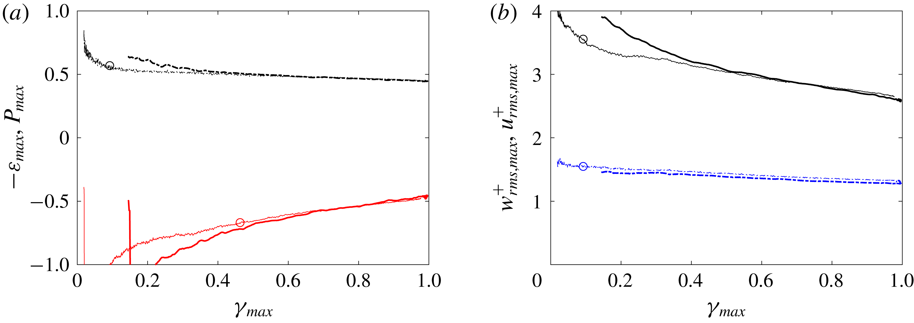
Figure 16. Turbulent-conditioned data in wall units versus $\unicode[STIX]{x1D6FE}_{max}$ . (a) Maximum TKE terms and (b) maximum turbulent intensities. $Tu_{0}=3\,\%$ (thick lines) and $Tu_{0}=2.5\,\%$ (thin lines with marker ○). $u_{rms,max}^{+}$ , $-\unicode[STIX]{x1D700}_{max}$ (——); $w_{rms,max}^{+}$ , $P_{max}$ (— ⋅ —).

4.1 Spatial structure of turbulence spots

The results from the two different ensemble averaging procedures will be compared: the unconditional ensemble and the turbulent ensemble as described in § 2.2.3. In the core of the turbulent patches, or more precisely in the overlap region of all the spots within the ensemble, both approaches are equivalent. Close to the spot boundaries, however, they differ appreciably. In the unconditional ensemble, the contribution of both laminar and turbulent data near the spot boundaries contaminate the results. When turbulent-conditioned data are used, streamwise and spanwise derivatives of mean quantities are difficult to compute near the spot periphery due to the irregularity of its boundaries and the lack of sufficient number of samples. For this reason, this approach will be used to compute the mean flow, the perturbation r.m.s. profiles, and turbulent production only.

The spots were selected for ensemble averaging based on their volume, which has to lie within a specified range. For the present study, the range is . In the simulation with  $T_{u}=2.5\,\%$ , a total of 58 spots satisfy this criterion and they appear within the streamwise extent $350<x-x_{0}<850$ . An example of the path of one such spot is shown in figure 17, which also shows the merging events that contribute to this spot history.

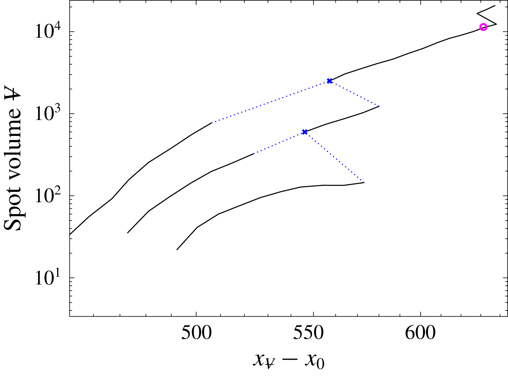
Figure 17. Example path of a spot which is included in the ensemble average from the dataset with $Tu_{0}=2.5\,\%$ , as a function of streamwise distance. As in figure 7 the blue crosses correspond to locations of spot merging, and the dotted lines connect two spot paths belonging to spots that undergo merging. The circle (pink online) highlights the spot streamwise location and volume that was selected for ensemble averaging.

The spot boundary resulting from ensemble averaging is depicted in figure 18, with its centre of volume located at . A new coordinate system $(\hat{x},\hat{z})$ is introduced with its origin located at. The ensemble-averaged spot exhibits all typical features of the instantaneous patches: a spot shape with pointed tip can be observed in the top view (figure 18 c); an overhang in the front of the spot, where turbulence does not reach the wall, is seen in the side view (figure 18 a). Slightly overhanging lateral wings are also seen in an end view (figure 18 b), although these are not very pronounced in the ensemble as they appear in individual spots. Red dashed lines and circles in the figure mark locations that will be discussed further.

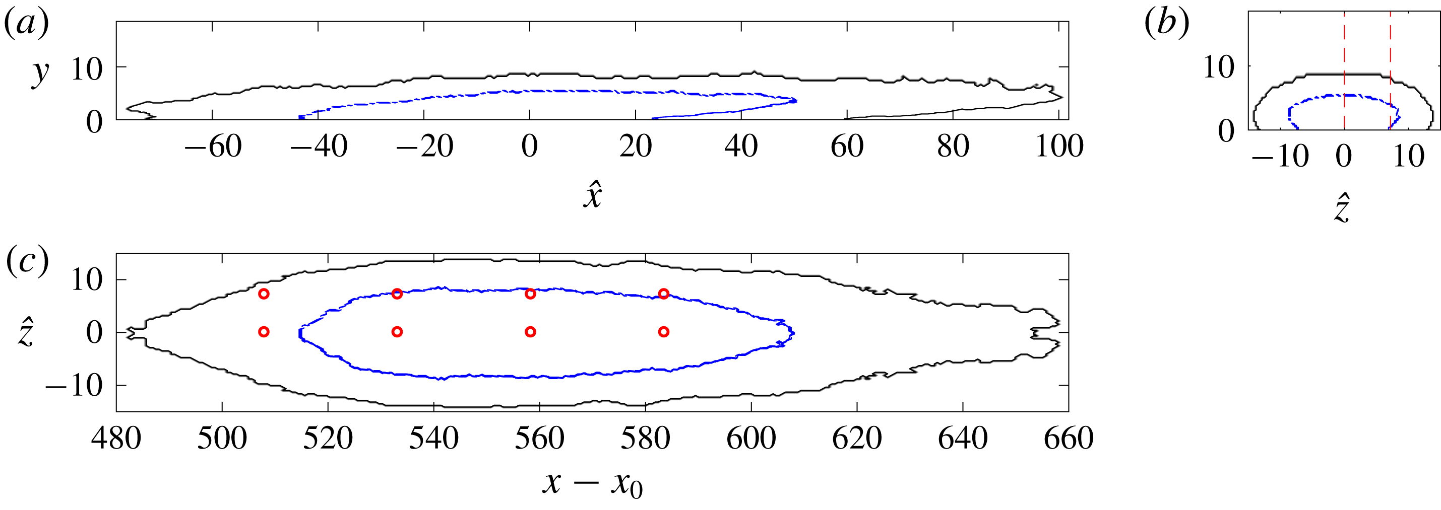
Figure 18. Visualization of the ensemble-averaged boundary of spots with

 in the dataset with $Tu_{0}=2.5\,\%$ . (a) Side view, (c) plan view and (b) end view of the boundary are plotted. The outer line is the boundary when at least 14 samples are included in the ensemble. The inner line marks the region which is shared by 90 % of the spots. Dashed lines and symbols mark locations that are examined in figures 23–25.

The skin-friction coefficient for the ensemble-averaged spot is plotted in figure 19, using both averaging techniques. Except near the rear, or upstream, boundary, the two approaches yield similar contours of $C_{f}$ throughout the spot. The value of $C_{f}$ reaches its peak close to the centre of the spot in both cases, and is significantly lower toward the front and lateral boundaries. Near the front part of the spot, $C_{f}$ is similar to the laminar values immediately downstream (figure 19 a).

Figure 19. Contours of skin-friction coefficient at the wall for spots with volumes

 for the dataset with $Tu_{0}=2.5\,\%$ . (a) Unconditional ensemble average superimposed with a black contour line that marks the boundary of the spot; (b) turbulent ensemble average.

In figure 20, the skin-friction coefficients at two spanwise locations within the spot, $\hat{z}=\{0,7.2\}$ , are compared to $C_{f}$ for fully turbulent flow. In the middle of the spot, the skin friction exceeds the fully turbulent level, although it decays below it near the front of the spot. The spot $C_{f}$ near the lateral edges, $\hat{z}=7.2$ , is also smaller than the turbulent level. In the unconditional ensemble (figure 20 a), the skin friction decays quickly at the upstream and downstream boundaries of the spot. This effect is due to the laminar contribution near the uneven edges of the ensemble members. The data from the turbulent ensemble (figure 20 b) show that $C_{f}$ remains high in the rear part of the spot. The corresponding Reynolds number based on the momentum thickness is given in figure 21.

Figure 20. Skin-friction coefficient for the ensemble-averaged spot in figures 18 and 19. The data are extracted along (solid line) $\hat{z}=0$ and (dash-dotted) $\hat{z}=7.2$ ; both locations are marked on figure 18. For reference, the turbulent-conditioned $C_{f}$ is also plotted (dotted grey line) for the corresponding $x-x_{0}$ range identified in figure 18. (a) Unconditional ensemble average with spatial filter; (b) turbulent-conditioned ensemble average. Vertical lines mark the nominal start and end of the spot at the respective spanwise locations. Circular symbols mark locations that are examined in figures 23–25.

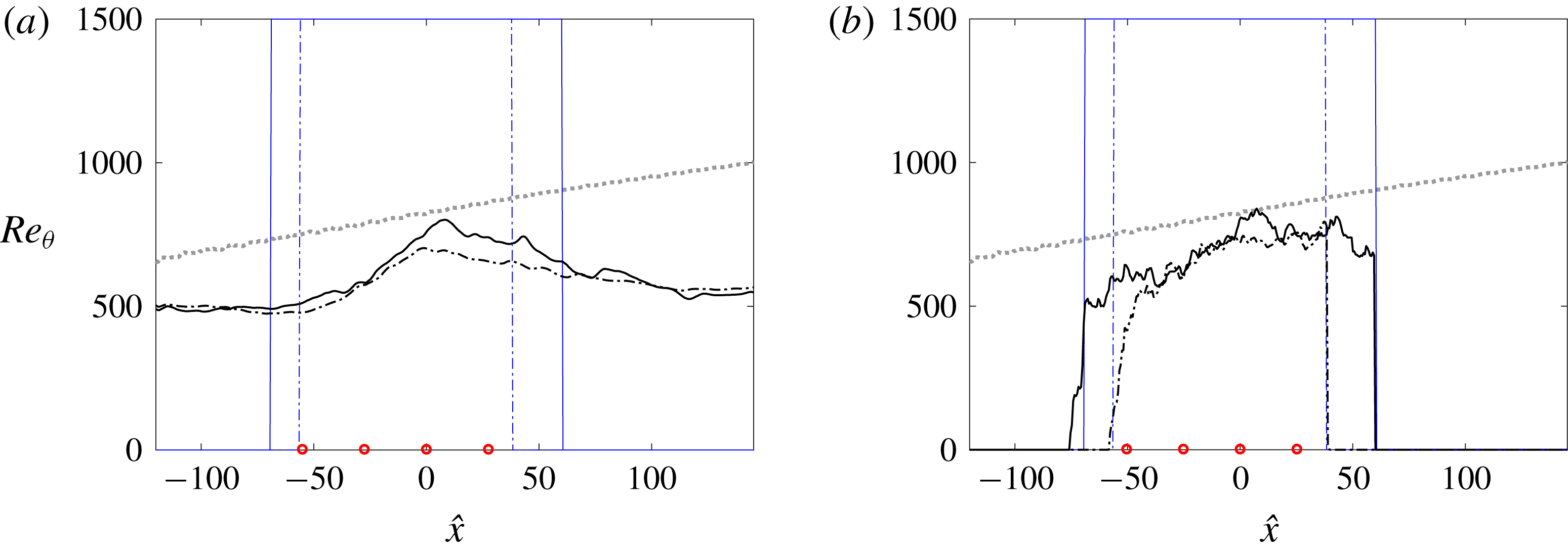
Figure 21. Reynolds number based on the momentum thickness for the ensemble-averaged spot in figures 18 and 19. The data are extracted along (solid line) $\hat{z}=0$ and (dash-dotted) $\hat{z}=7.2$ ; both locations are marked on figure 18. For reference, the turbulent-conditioned $Re_{\unicode[STIX]{x1D703}}$ is also plotted (dotted grey line) for the corresponding $x-x_{0}$ range identified in figure 18. (a) Unconditional ensemble average with spatial filter; (b) turbulent-conditioned ensemble average. Vertical lines mark the nominal start and end of the spot at the respective spanwise locations. Circular symbols mark locations that are examined in figures 23–25.

When the skin friction is further averaged in the spanwise direction (figure 22), it exhibits a plateau in the rear of the spot. Also, the elevated friction near the core has been counterbalanced by the lower $C_{f}$ near the periphery. Spots with lower volumes exhibit lower skin friction, as demonstrated by a comparison of figure 22(a,b).

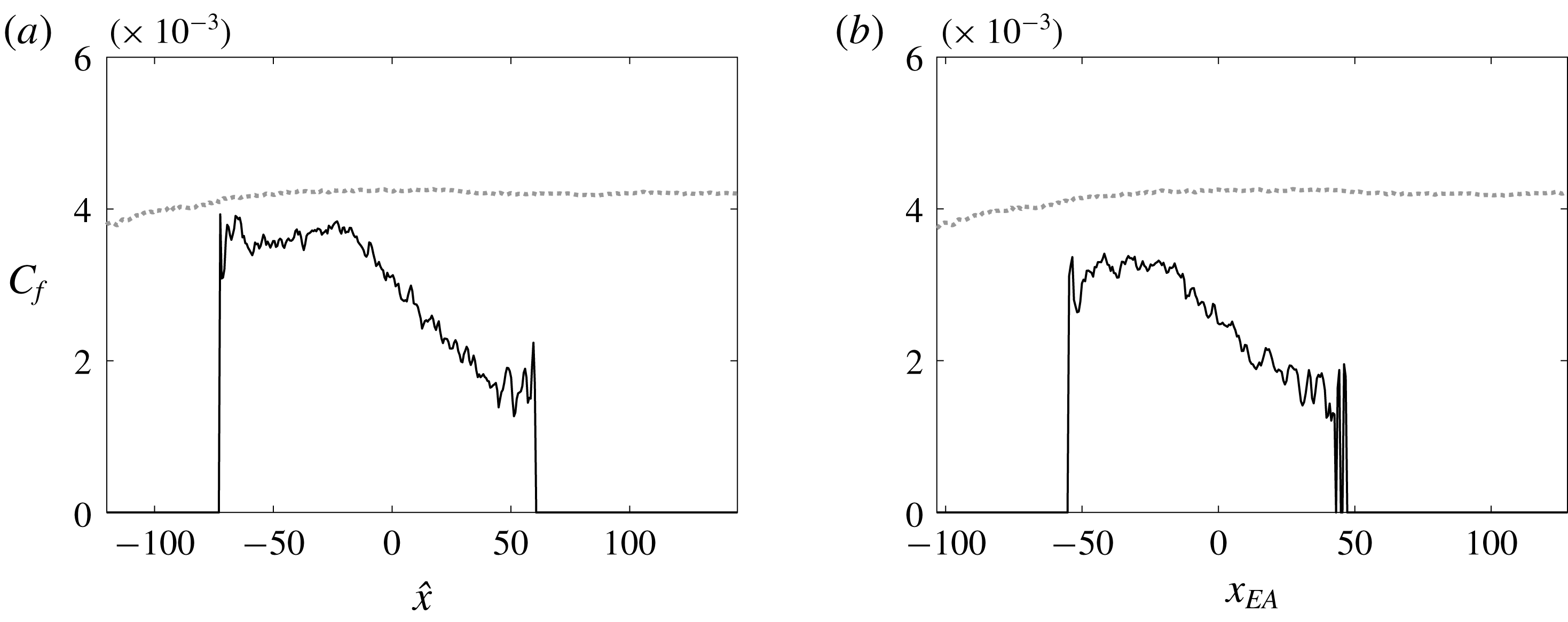
Figure 22. Spanwise average $C_{f}$ evaluated from the turbulent ensemble-averaged spot. The figure compares spots whose volumes lie in the range (a)

 and (b) and

 for the dataset with $Tu_{0}=2.5\,\%$ . For reference, the turbulent-conditioned $C_{f}$ is also plotted (dotted grey line) for the corresponding $x-x_{0}$ range identified in figure 18.

Mean streamwise velocity profiles at eight locations, four streamwise and two spanwise positions, are shown in figure 23. The top row (a–d) is from the unconditional ensemble, and the bottom one (e–h) is from the turbulent ensemble. For comparison, profiles form the turbulent boundary layer farther downstream, at $Re_{\unicode[STIX]{x1D703}}=1223$ are included (dashed, red online).

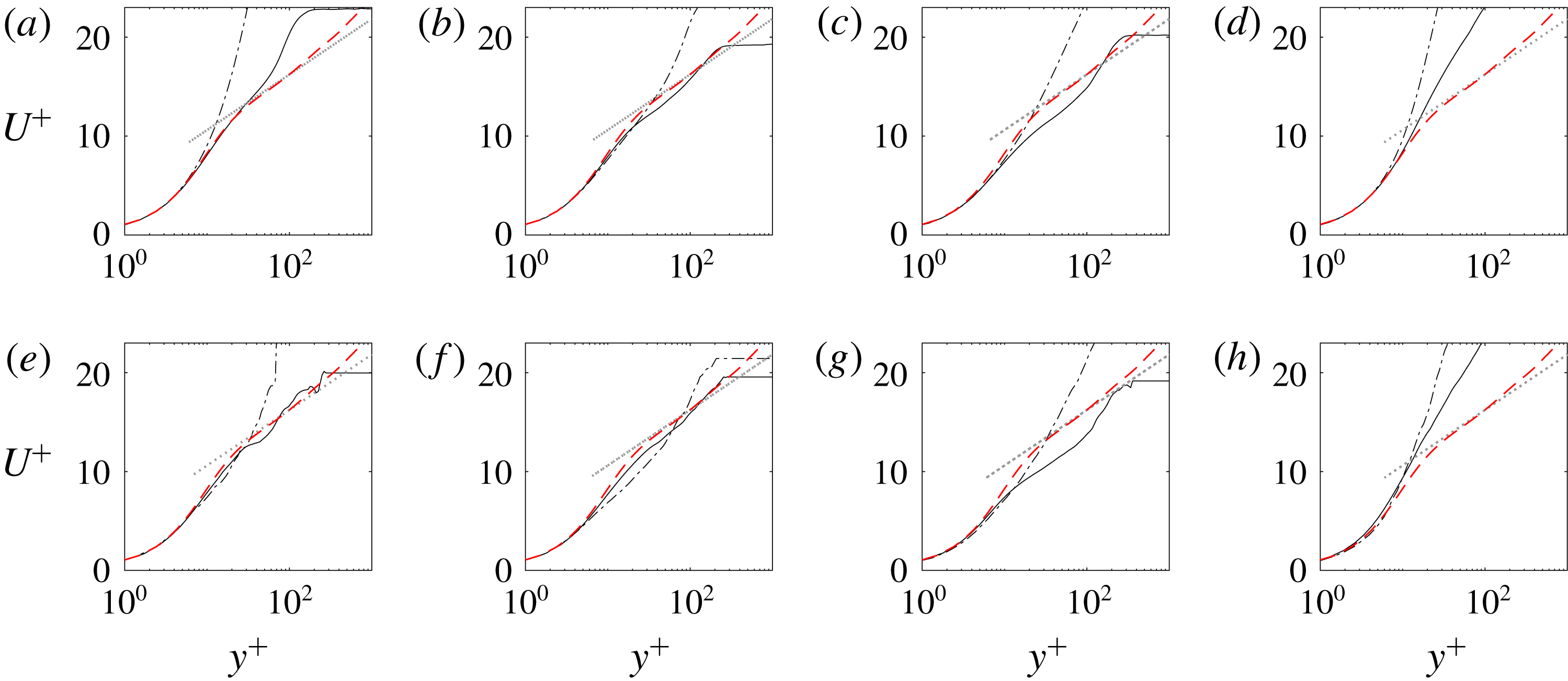
Figure 23. Mean streamwise velocity versus wall-normal distance in wall units, for spots with

 for the dataset with $Tu_{0}=2.5\,\%$ . Profiles are evaluated at the locations marked in figure 18; (solid) $\hat{z}=0$ and (dash-dotted) $\hat{z}=7.2$ . (a–d) Unconditional and (e–h) turbulent ensemble. For reference, the log law (dotted line) and the turbulent-conditioned data at $Re_{\unicode[STIX]{x1D703}}=1223$ are also shown (see figure 8) (dashed line, red online).

Results at the centreline positions ( $\hat{z}=0$ ) are virtually identical when evaluated using the unconditional or turbulent ensemble (compare solid lines in figure 23(a–h), except panels (a) and (e)). The differences between the two approaches are most pronounced in the upstream locations of the spot, in panels (a) and (e). They are due to the contribution of laminar flow data for the unconditional ensemble (panel a), and the lower sample size in the turbulent ensemble (panel e) which leads to more fluctuating profiles. For off-centre positions, the differences between the two averaging procedures are pronounced in the two most upstream locations (panels a,b and e,f).

The velocity profiles using the unconditional ensemble, at $\hat{z}=7.2$ (dash-dotted lines in panels a–d), are elevated beyond the log law for turbulent flow at all streamwise positions. To eliminate the effect of including any laminar regions in the ensemble, the same profiles are plotted in panels (e,f) using the turbulent ensemble. The same trend generally persists, which confirms that the effect is due to the turbulence in this region being non-equilibrium. The elevated profile is also in agreement with the skin-friction curve (figure 20), which is below the fully turbulent value at all off-centre locations.

The mean velocities at the plane of symmetry $\hat{z}=0$ (solid lines in figure 23) show an interesting behaviour: proceeding from the rear to the front of the spot (a–d), the profile is initially elevated, then matches the log law, becomes more depressed and finally again breaches towards the laminar state. In the turbulent ensemble (e,f), the first two locations match the log law, which indicates that the turbulence is developed in those regions. Downstream, the profile subsequently dips below the log law, which is generally associated with local drag increase. This effect is consistent with figure 20 that shows the highest friction coefficient at this streamwise location. Finally the profile becomes higher than the log law, in the region where the friction coefficient decays below the equilibrium turbulent level. These results suggest that the dynamics of the flow in the core of the spots are similar to fully developed turbulent boundary layers, but that the wingtips and front region differ. This view is supported by further evidence from other flow quantities.

For the same locations within the spot, figure 24 shows profiles of the root-mean-square velocity perturbations. Only the turbulent ensemble is plotted, and the profiles are compared to the turbulent conditional average. The top row (a–d) corresponds to the line of spanwise symmetry, and there the profiles agree with the turbulent data except near the front of the spot where $u_{i,rms}^{\prime +}$ from the turbulent ensemble are elevated. The same tendency for the stresses to overshoot the turbulent data are observed at all off-centre positions (e,f). While the difference from the fully turbulent curves decreases near the back of the spot (e), an agreement is never reached. The results support the view that only a core region within the spot has reached the same statistical state of fully turbulent flow, while non-equilibrium effects remain pronounced near the spot periphery. The higher values of all three root-mean-square components relative to fully turbulent boundary-layer data are in part due to the lower friction velocity at the spot side and front edges. The overshoot in $u_{rms}^{\prime +}$ is, however, appreciably larger than the other two components, which is akin to characteristics of the laminar state that preceded spot inception and where $u^{\prime }$ is generally much higher than the other components due to the Klebanoff streaks. The turbulence is thus anticipated to be less developed in those regions, and to be dominated by a $u^{\prime }$ amplification mechanism without sufficient dissipation or redistribution to the other components. The present results also provide a finer grain interpretation of the conditionally averaged data in § 3, where $u_{rms}^{\prime }$ is elevated relative the turbulent data while the other components were in closer agreement (cf. figure 14).

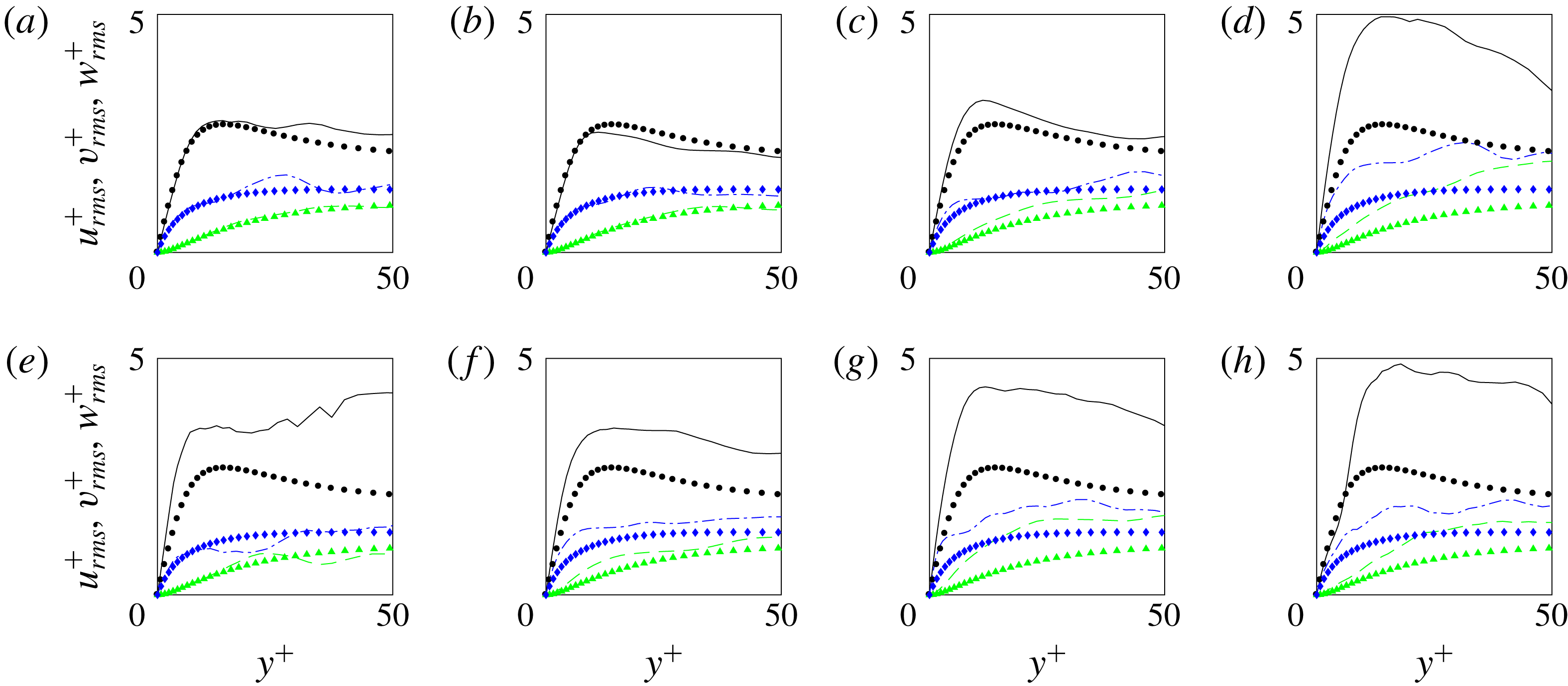
Figure 24. Turbulent ensemble-average r.m.s. values for the streamwise, spanwise and wall-normal velocity component (lines, top to bottom in each panel) in plus coordinates for spots with volumes

 for the dataset with $Tu_{0}=2.5\,\%$ at $\hat{x}=\{-50.1,-24.9,0.28,25.5\}$ (left to right) and $\hat{z}=\{0,7.2\}$ (top to bottom) marked in figure 18. The symbols correspond to turbulent conditional average at the same streamwise locations.

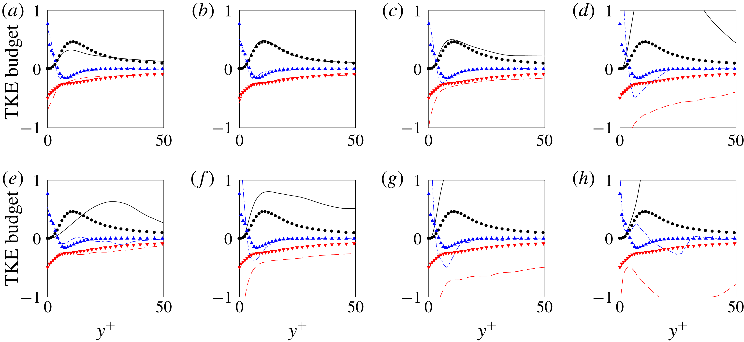
Figure 25. Unconditional ensemble-averaged TKE terms (solid black line: production; dashed red line: pseudo dissipation; dashed-dotted blue line: viscous diffusion) for spots with volumes

 for the dataset with $Tu_{0}=2.5\,\%$ at $\hat{x}=\{-50.1,-24.9,0.28,25.5\}$ (left to right) and $\hat{z}=\{0,7.2\}$ (top to bottom) marked in figure 18. The symbols correspond to turbulent conditional average at the same streamwise locations.

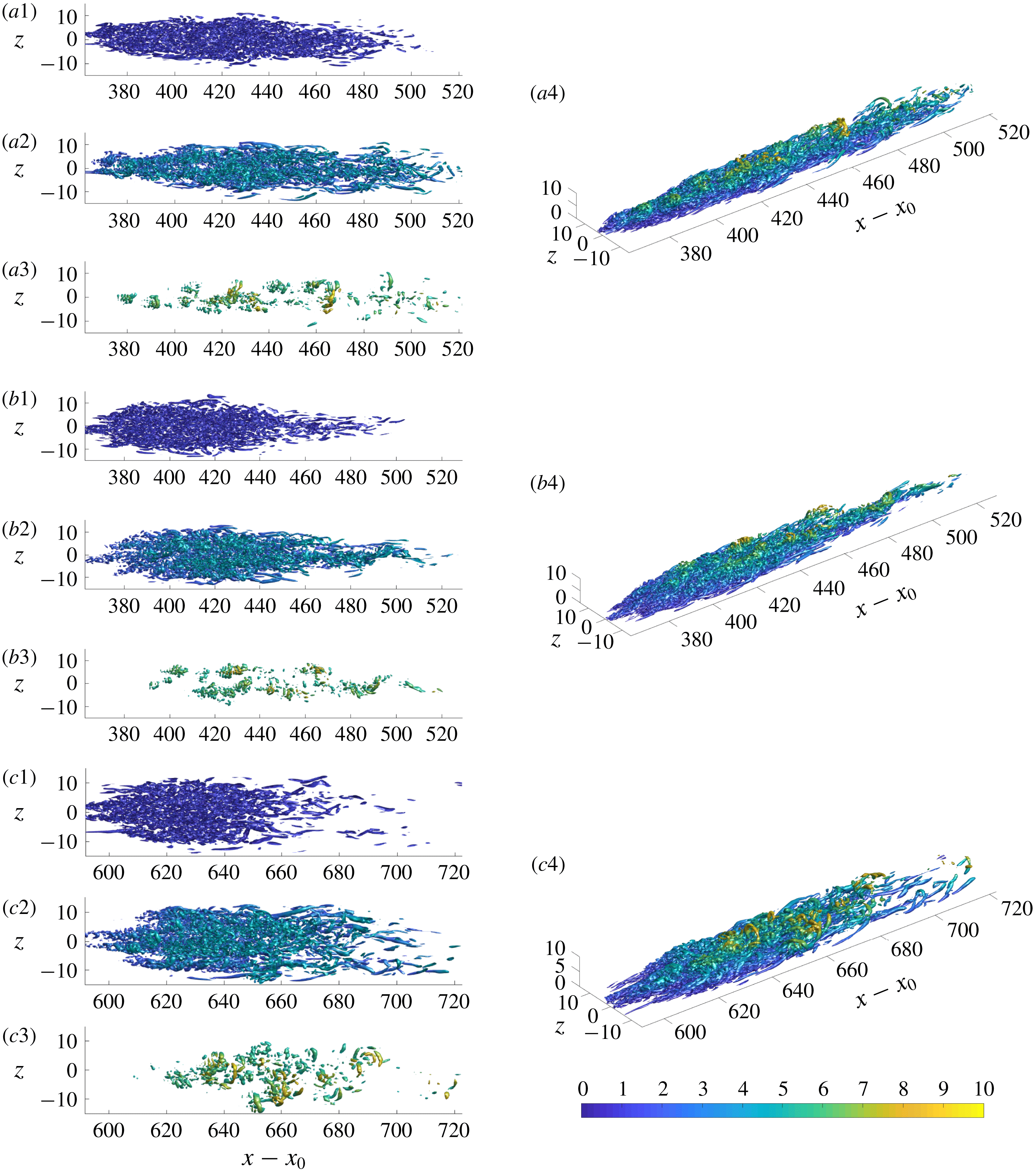
Figure 26. Instantaneous vortex visualization using the $\unicode[STIX]{x1D706}_{2}$ -criterion for three spots $\{a,\!b,\!c\}$ that contributed to the ensemble average. Spot volumes lie within the range

 for the dataset with $Tu_{0}=2.5\,\%$ . The vortical structures are coloured by wall-normal distance, and are visualized in the wall-normal ranges (1) $0\leqslant y/\unicode[STIX]{x1D6FF}_{0}\leqslant 1.5$ , (2) $1.5\leqslant y/\unicode[STIX]{x1D6FF}_{0}\leqslant 5$ , (3) $5\leqslant y/\unicode[STIX]{x1D6FF}_{0}\leqslant 10$ , and (4) the entire wall-normal extent $0\leqslant y/\unicode[STIX]{x1D6FF}_{0}\leqslant 10$ in a three-dimensional view.

The difference in the state of the turbulence with spatial location, and in particular between the core and periphery of the spot, can be further examined by contrasting terms in the turbulence kinetic energy equation. These were evaluated from the unconditional ensemble only, and are shown in figure 25. The production, dissipation and diffusion terms in the core region of the spot (b,c) show the expected behaviour for a fully turbulent boundary layer. They are, however, much higher near the downstream edge (d) and the lateral edges of the spot (f–h). Both the production and dissipation are large in those regions, which is in part due to scaling by a lower value of the local friction velocity, but also due to the non-equilibrium nature of the turbulence. The shift of the production curve towards higher values of $y^{+}$ is also notable, and is a symptom of the production being driven by large-scale motions near the lateral sides of the spot.

Figure 26 provides vortex visualizations of three turbulent spots that were included in the ensemble average, but all spots have been inspected and were found to exhibit similar features. These visualizations help explain some of the trends just discussed. From ensemble averaging, fully developed turbulence could only be found around the centre of the spot. It is at these locations that we observe hairpin vortices that reach far away from the wall (panels a3, b3 and c3 in figure 26) as well as exhibiting small-scale vortical motions all the way to the wall (panels a1, b1 and c1 in figure 26). The front part and the lateral wings of the turbulent spots are dominated by large-scale streamwise-oriented vortices. In these regions of the ensemble-averaged spot, increased turbulent production is observed.

The structure of the spots, which can be difficult to glean from instantaneous realizations, becomes more evident by examining the ensemble. In figure 27, contours of the unconditional ensemble-average velocities are shown in side views. The streamwise component captures the fuller velocity profile in the centre of the spot, and how it gives way to laminar velocities in the rear and front parts. The vertical velocity shows an interesting trend: it is positive only in a limited region near the spot centre, where the boundary layer is closest to a fully turbulent state; towards the rear and front parts of the spot, the vertical velocity is negative, which is required in order to transition the streamwise velocity profiles from the laminar to a fuller turbulent shape. The spanwise velocity points outward in the near-wall region. The mean motion within the spot can then be viewed as a large-scale engulfment of fluid near the free-stream edge, and displacing it downwards towards the wall. The engulfed fluid becomes part of the turbulence in the core of the spot. Once the downward flow impinges onto the bottom wall, it spreads outward along the wings.

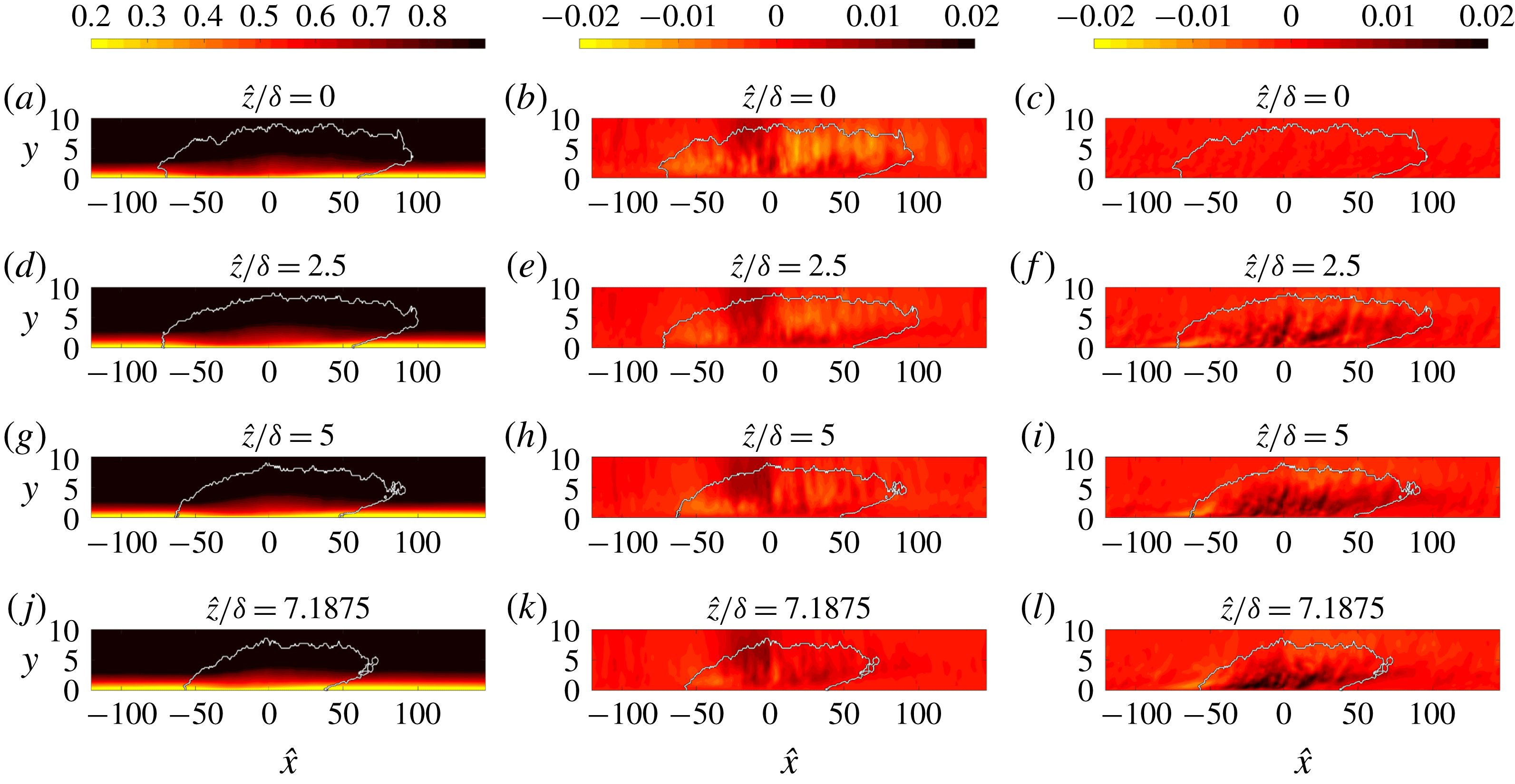
Figure 27. Contours of the unconditional ensemble (a,d,g,j) $\overline{u}$ , (b,e,h,k) $\overline{v}$ and (c,f,i,l) $\overline{w}$ for spots with volumes

 for the dataset with $Tu_{0}=2.5\,\%$ at $\hat{z}/\unicode[STIX]{x1D6FF}=\{0,2.65,5,7.2\}$ .

The turbulent ensemble streamwise velocity and root-mean-square perturbation are plotted in figure 28 at two wall-parallel planes. The mean velocity within the spot is lowest near the lateral edges (a,c), where the mean velocity profile retains laminar characteristics as previously remarked in connection with figures 23–25. The root-mean-square of the streamwise velocity perturbation in these regions, and towards the front of the spot, is larger than in the core of the spot (figure 28 b,d). Hence, the flow in these regions can be best characterized as being in a non-equilibrium turbulent state.

Figure 28. Contours of the turbulent ensemble of (a,c) $\overline{u}$ and (b,d) $u_{rms}^{\prime }$ for spots with volumes

 in the dataset with $Tu_{0}=2.5\,\%$ . The plane views are extracted at (a,b) $y/\unicode[STIX]{x1D6FF}=1.46$ and (c,d) $y/\unicode[STIX]{x1D6FF}=0.43$ .

Turbulent production is plotted in figure 29. The production peaks in the tip (front) and the wings of the turbulent spot, and is largest in the same areas where the root-mean-square values of the streamwise velocity are highest. There are no qualitative differences between results from unconditional and turbulent ensembles in those regions (figure 29 a–d), and as such the results are not appreciably contaminated by the details of the averaging procedure.

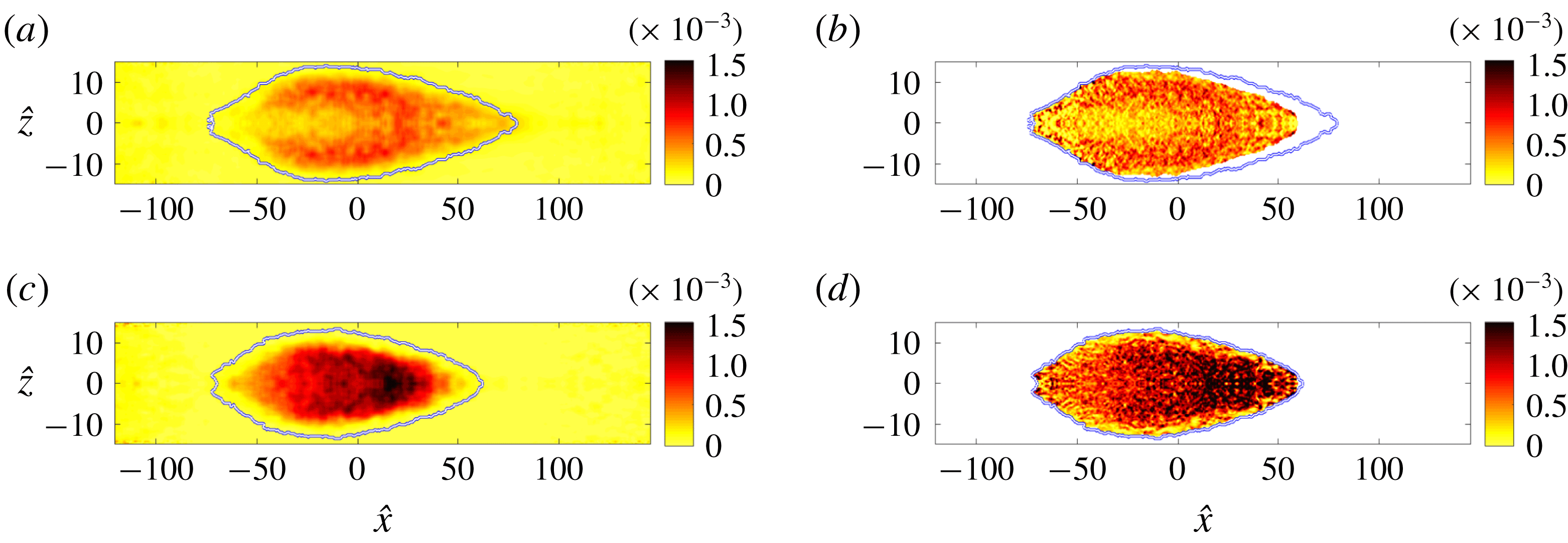
Figure 29. Contours of turbulent production ${\mathcal{P}}$ , normalized by the free-stream velocity and inlet boundary-layer thickness. Data from case with $Tu_{0}=2.5\,\%$ at two different planes (a,b) $y/\unicode[STIX]{x1D6FF}=1.46$ and (c,d) $y/\unicode[STIX]{x1D6FF}=0.43$ . (a,c) Unconditional ensemble; (b,d) turbulent ensemble.

The above results demonstrate that the turbulence characteristics within the spot vary in space. Near the periphery, averaged terms in its kinetic energy equation deviate appreciably from those of turbulent boundary layers. Near the core, however, the statistics relax towards those of fully turbulent conditions.

4.2 Additional considerations: spot size and free-stream turbulence intensity

In order to illustrate the effect of spot size on its spatial structure, two additional volume ranges were examined, and . The two ranges are progressively smaller spots than those studied above. In all cases, a similar number of spots was used for ensemble averaging. Qualitatively, the ensemble-averaged spot shape remains similar to figure 18, and hence is not shown.

Consistent with results from larger spots, terms from the TKE budget within the smaller spot are higher than the levels typically observed in fully turbulent boundary layers. The r.m.s. perturbation levels (not shown) are also larger in the young spots than in fully turbulent boundary layers. The production is reported as an example in figure 30. It is high throughout the spot, at levels commensurate with those recorded near the lateral wings and front of the larger spots in figure 29. The core region where the turbulence is less energetic and is statistically similar to fully turbulent boundary layers is entirely absent at the smallest volume (figure 30 b,d).

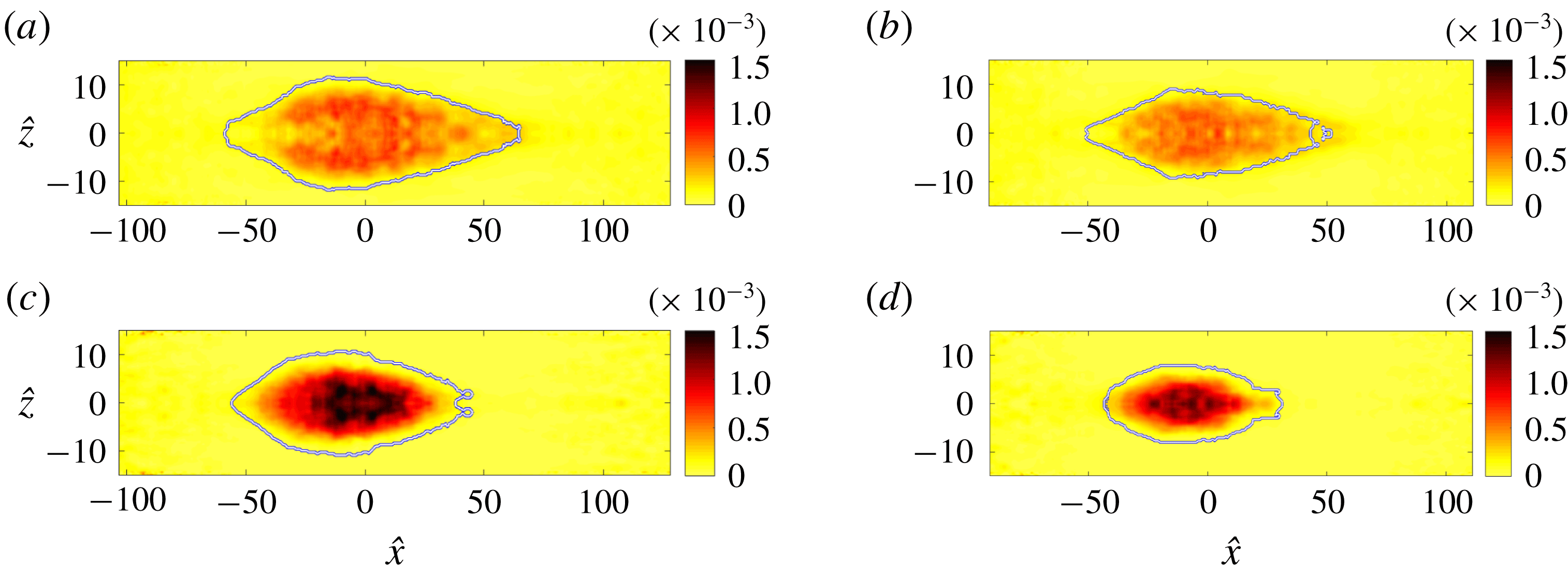
Figure 30. Contours of turbulent production ${\mathcal{P}}$ , normalized by the free-stream velocity and inlet boundary-layer thickness, for spots with volumes (a,c)

 and (b,d)

. Data from case with $Tu_{0}=2.5\,\%$ at two different planes (a,b) $y/\unicode[STIX]{x1D6FF}=1.46$ and (c,d) $y/\unicode[STIX]{x1D6FF}=0.43$ .

A similar analysis of ensemble-averaged spots was performed for the dataset with higher free-stream turbulence intensity, $Tu_{0}=3\,\%$ . In this case, significantly fewer spots could be used for averaging, and hence corresponding results are not treated in much detail here. Despite the low sampling rate, the results and the spatial structure of the turbulence statistics within the spots were qualitatively similar to the data from the lower intensity case. Figure 31, for example, shows the turbulence production and the root-mean-square of the streamwise velocity perturbation. It confirms that the turbulence activity is most pronounced in the front region and lateral periphery of the spot.

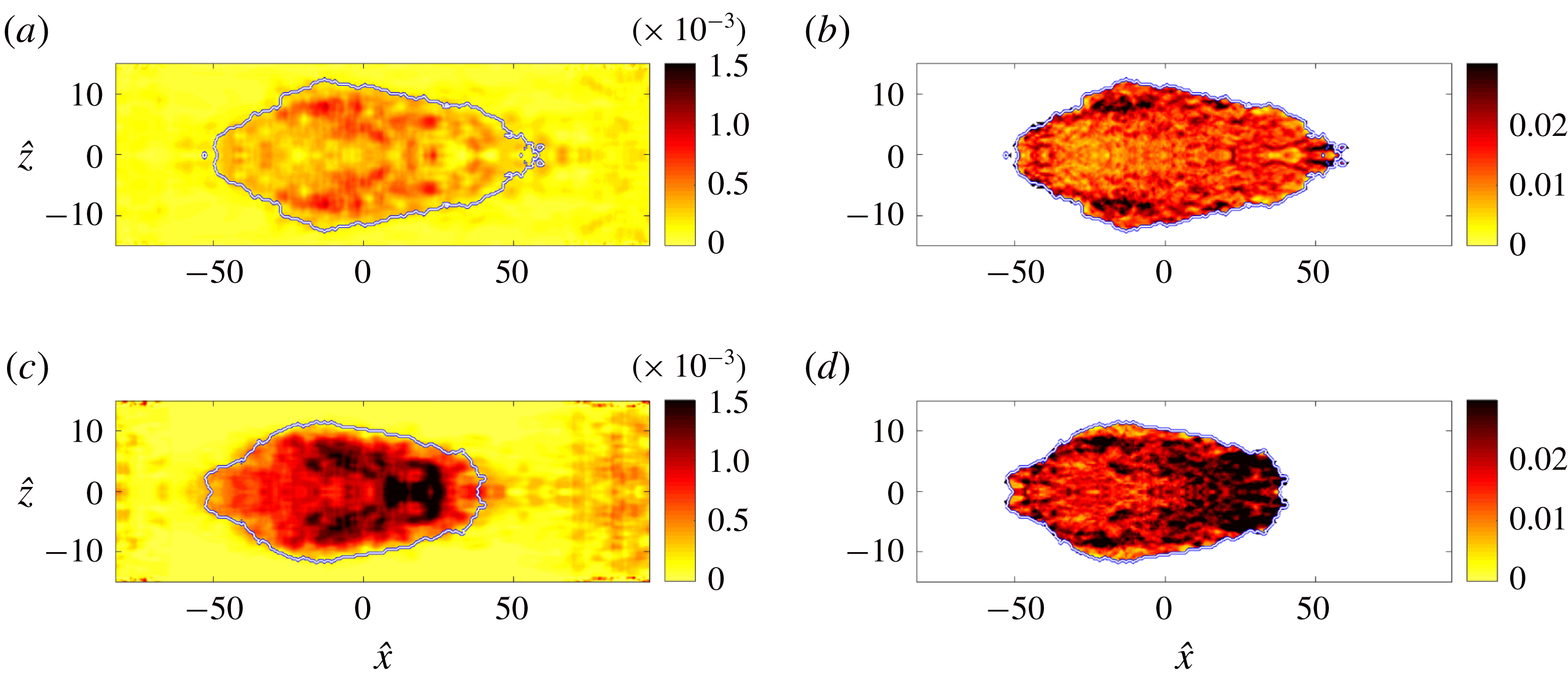
Figure 31. (a,c) Contours of the unconditional ensemble TKE production ${\mathcal{P}}$ , normalized by the free-stream velocity and inlet boundary-layer thickness, for spots with volumes

 for the dataset with $Tu_{0}=3\,\%$ . (b,d) Contours of the turbulent ensemble $u_{rms}^{\prime }$ for spots with volumes

 for the dataset with $Tu_{0}=3\,\%$ . The planes are located at (a,b) $y/\unicode[STIX]{x1D6FF}=1.46$ and (c,d) $y/\unicode[STIX]{x1D6FF}=0.43$ .