3.1. Geometry

For fixed $\varepsilon$ and $N$, when the tip-speed ratio $\lambda$ and vortex strength parameter $\eta$ are varied, different vortex geometries are obtained. These geometries are illustrated for a fixed $\eta$ and different $\lambda$ in figures 4 and 5.

Figure 4. Vortex geometry for a two-bladed rotor in wind turbine regimes; (a) $\lambda =3.3$, (b) $\lambda =4.3$, (c) $\lambda =5.1$, (d) $\lambda =6.1$. For all cases $\eta = 0.05$ and $\varepsilon = 0.01$.

Figure 5. Vortex geometry for a two-bladed rotor in helicopter regimes; (a) $\lambda =-10$, (b) $\lambda =\infty$, (c) $\lambda =19$, (d) $\lambda =11$. For all cases $\eta = 0.05$ and $\varepsilon = 0.01$.

Two main types of solutions are obtained according to the behaviour of the solution away from the rotor: solutions in the wind turbine regime for which the vortex structure expands and goes upwards (figure 4); solutions in the helicopter regime for which the vortex structure contracts and goes downwards (figure 5). This corresponds to the two domains of parameters, which are indicated in figure 6 for $\varepsilon = 0.01$ and $N=2$ on either side of the grey region where no solution has been obtained.

Figure 6. Map of the rotor regimes as a function of $\lambda$ and $\eta$. The grey region represents the region where no solution has been obtained. On the left, helicopter regimes: the wake contracts and is advected downwards. On the right, wind turbine regimes: the wake expands and is advected upwards. In both regimes, the dashed line corresponds to the boundary of the domain where the tip vortices are on either side of the rotor plane. The other boundary of that domain is the grey region.

Before describing the geometry of the vortices close to the rotor, let us first look at the characteristics of the far wake. By construction, the tip vortices form perfect helices in the far wake. The radius $R_{FW}$ and pitch $h_{FW}$ of these helices are shown in figure 7 for the parameters of figure 6. By convention, we have chosen the pitch to be positive when the vortices go upwards, and negative when they go downwards. We can see that both the wake contraction in the helicopter regime and the wake expansion in the wind turbine are reduced as the tip-speed ratio $|\lambda |$ decreases. An opposite tendency is by contrast observed for the far-wake helix pitch that increases with $|\lambda |$.

Figure 7. Contour maps of the far-wake helix characteristics for $\varepsilon = 0.01$; $N=2$, non-dimensionalized by $R_b$. (a) Radius $R_{FW}/R_b$; (b) pitch $h_{FW}/R_b$. By convention, $h_{FW}$ is negative (respectively positive) when the vortices are advected downwards (respectively upwards). The dashed lines represent the theoretical formulae (3.3a) (yellow) and (3.3b) (red).

An estimate for $h_{FW}$ can be deduced from simple arguments. As the helical structure is stationary (in the frame rotating at the angular speed $\varOmega _R$), its rotation must be balanced by its axial displacement, that is $V_{FW}/ \Omega _{FW} = - h_{FW}/(2{\rm \pi} )$ (assuming $\varOmega _{FW}<0$). An approximation to the axial displacement speed $V_{FW}$ can be obtained from the displacement speed of a double array of opposite point vortices separated by a distance $h_{FW}/N$ in a background axial flow $V_{\infty }$, that is $V_{FW}= -N \varGamma /(2 h_{FW}) + V_{\infty }$ in the wind turbine regimes and $V_z = N \varGamma /(2 h_{FW}) + V_{\infty }$ in the helicopter regimes. If we neglect the self-induced rotation of the structure, that is assume that $\Omega _{FW}\approx - \Omega _R$, the condition of stationarity then gives

(3.1a)\begin{gather} h_{FW} = \frac{2{\rm \pi}}{\varOmega_R} \left(\frac{N\varGamma}{2 h_{FW} } + V_{\infty}\right), \quad \text{for helicopter regimes}\ (h_{FW} <0), \end{gather}

(3.1b)\begin{gather}h_{FW} = \frac{2{\rm \pi}}{\varOmega_R} \left(-\frac{N\varGamma}{2 h_{FW} } + V_{\infty}\right) , \quad \text{for wind turbine regimes}\ (h_{FW} >0). \end{gather}

This gives a second-order equation for $X=h_{FW}/R_b$ of the form

(3.2)\begin{equation} X^{2} - \frac{2{\rm \pi}}{\lambda} X \pm N {\rm \pi}\eta =0, \end{equation}

where the sign $-$ is for helicopter regimes, and the sign $+$ for wind turbine regimes. The adequate solution for each case is

(3.3a)\begin{gather} h_{FW}/R_b = \frac{\rm \pi}{\lambda} - \sqrt{\frac{{\rm \pi}^{2}}{\lambda^{2}} + N {\rm \pi}\eta} ,\quad \text{for helicopter regimes}\ (h_{FW} <0), \end{gather}

(3.3b)\begin{gather}h_{FW}/R_b = \frac{\rm \pi}{\lambda} + \sqrt{\frac{{\rm \pi}^{2}}{\lambda^{2}} - N {\rm \pi}\eta} ,\quad \text{for wind turbine regimes}\ (h_{FW} >0). \end{gather}

These contours are plotted with dashed lines in figure 7(b). We can see that these formulae provide a reasonably good approximation of $h_{FW}/R_b$, especially for small $\eta$.

The wind turbine regime is associated with large values of $1/\lambda$. It also corresponds to the so-called windmill brake regime of helicopters in rapid descent flight. In this regime, the vortices move in the direction of the external wind, and the vortex structure expands. As seen in figure 8(b), the radius of the structure increases monotonously up to its far-wake value. By contrast, the vortex pitch does not seem to change much along the structure at least as long as $\lambda$ is not too large (figure 9b). The most interesting feature is the existence, for each $\eta$, of a critical value of $\lambda$ above which the tip vortices are first emitted downwards before being advected upwards.This transition is materialized by a dashed line on the right of the grey region in figure 6. As $\lambda$ gets larger, the expansion continues to increase and finally gets too large to fit in the computation domain. This provides the limit of existence of the wind turbine solutions.

Figure 8. Radial position of the wake in the axial direction for different tip-speed ratio values. With $\eta =0.05$, $\varepsilon =0.01$ and $N=2$. (a) Helicopter regimes. (b) Wind turbine regimes.

Figure 9. Evolution of the local pitch along the wake for different tip-speed ratio values. With $\eta =0.05$ and $\varepsilon =0.01$. (a) Helicopter regimes. (b) Wind turbine regimes. By convention, $h_{FW}$ is negative (respectively positive) when the vortices are advected downwards (respectively upwards).

The change of direction of the vortex emission as $\lambda$ increases has been observed experimentally. In figure 10(a,c) we visualize using dye the time-averaged trajectories of the vortices in a rotor side view for values of $\lambda$ before and after the transition. We clearly see on the bottom view obtained for $\lambda =11.2$ that the trajectory of the tip vortex goes below the rotor plane. Unfortunately, vortex circulation and core size have not been measured in the experiment, so we cannot perform a quantitative comparison. Nevertheless, figure 10 demonstrates that we can obtain a good agreement for the geometry with the numerical model for similar values of $\lambda$.

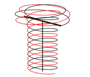
Figure 10. Time-averaged dye visualization of the wake behind half of the rotor plane in a wind turbine configuration at $\lambda = 7.23$ (a,b) and $\lambda =11.2$ (c,d) (from Quaranta Reference Quaranta2017). (a,c) Qualitative comparison of the wake geometry with the numerical model for wind turbine configuration at high tip-speed ratio (up: $\lambda =8$, down: $\lambda =10$; $\eta = 0.02$, $\varepsilon =0.01$). The rotor disc is represented in black dashed line. In black solid line, the projection of the tip vortices and, in red, their radial evolution.

In the helicopter domain of parameters (left side of the grey region in figure 6), we cover the normal flight conditions of a helicopter: climbing flight for negative $1/\lambda$, hovering for $1/\lambda =0$ and weak descent flight for positive (and small) values of $1/\lambda$. In all these cases, the vortex structure matches away from the rotor a helical structure that moves downwards, although the external wind is downwards for negative $\lambda$ and upwards for positive $\lambda$.

The main modifications of the geometry as $\lambda$ varies are observed close to the rotor plane. In figures 8(a) and 9(a) we display the variation in the wake of the radius and pitch of the vortex structure, respectively. As already mentioned above, we can observe in figure 8(a), that the contraction of the vortex structure becomes more important as $1/\lambda$ increases. As for the wind turbine regime, we observe that there exists a critical value of $1/\lambda$ above which tip vortices are no longer emitted towards its far wake, but in the opposite direction. This transition is indicated by a dashed curve on the left of the hatched region in figure 6. For values of $1/\lambda$ larger than this critical value, the vortices go upwards before being advected downwards. Accordingly, the local pitch changes sign as we move along the structure: it is positive when the vortices move upwards close to rotor, and becomes negative afterwards when vortices start to be advected downwards (see figure 9a).

It is interesting to note that the transition curve is close to the line $1/\lambda =0$ but not identical to this line. For small $\eta$ (low loading), this transition occurs in a climbing flight configuration, whereas this transition is observed in the descent flight regime for large $\eta$ (strong loading). As $1/\lambda$ is increased above the transition, the vortex excursion above the rotor plane becomes more important. It becomes more and more difficult to follow the solution as the number of turns above the rotor plane grows as $1/\lambda$ increases.

For all the parameters tested, we have not found any overlap between the wind turbine domain and the helicopter domain. However, we cannot exclude this possibility if a larger computational domain is considered for wind turbine solutions or if helicopter solutions are continued further.

3.2. Induced velocities

For applications, especially the design of rotors, it is useful to know the velocity field induced by the vortex structure. In this section, we provide the induced velocity field for four different configurations typical of each identified flow regime. We fix $\eta$, $\varepsilon$ and $N$ ($\eta =0.05$, $\varepsilon =0.01$, $N=2$) and consider different values of $\lambda$ ($\lambda =-20$, $\lambda =11$, $\lambda =6.2$, $\lambda =4.3$). For convenience, we normalize the induced axial velocity by the outer velocity $V_{\infty }$, and the induced azimuthal velocity by the azimuthal velocity $\varGamma / (2{\rm \pi} r)$ of a vortex filament of circulation $\varGamma$.

In figure 11 are shown contours plots of each velocity component in the rotor plane for each case. In figure 12 we compare, for each case and each component, the induced velocity on the blade (black dashed line), the mean (azimuthal average) induced velocity in the rotor plane (black solid line) and the mean induced velocity in the far wake (red solid line).

Figure 11. Induced velocity contours in the rotor plane ($z=0$ plane) for $\eta = 0.05$, $\varepsilon = 0.01$, $N=2$ and various $\lambda$ ($\lambda = -20, 11, 6.2, 4.3$); (a–d) $V_z^{ind} /V_{\infty }$, (e–h) $V_{\phi }^{ind} 2{\rm \pi} r/\varGamma$.

Figure 12. Induced velocity profiles. (a,c,e,g) Axial velocity $V_z^{{ind}}/V_{\infty }$, (b,d,f,h) azimuthal velocity $V_{\phi }^{{ind}} 2{\rm \pi} r/\varGamma$ for various values of $\lambda$ and $\eta =0.05$, $\varepsilon =0.01$ and $N=2$. In black, the profiles in the rotor plane (dashed: on the blade, solid: azimuthal average), in red, the azimuthal average in the far wake.

The first point to emphasize is the axisymmetric character of the induced flow (figure 11). In the rotor plane, both velocity components are almost axisymmetric. In the rotor plane, the difference between the azimuthally averaged field and the local field is mainly concentrated in the close neighbourhood of the vortices (see figure 11). This is also clearly visible in figure 12, where we can see that the velocity on the blade (black dashed line) departs from its azimuthal average (black solid line) at specific locations: at the blade tip, and at the location where one vortex crosses the rotor plane ($r/R_b \approx 0.6$ for $\lambda =11$; $r/R_n\approx 2.1$ for $\lambda =6.2$).

The azimuthally averaged profiles of the induced velocity possess interesting features. As soon as we are outside the vortex structure, both the axial and the azimuthal components vanish. This is true in the far field and in the rotor plane as well (see figure 12). In the far field, both components are also constant inside the vortex structure. This is in agreement with known properties of the induced velocity of infinite helices (see Hardin Reference Hardin1982). In the rotor plane, we can note that both components are also constant inside the vortex structure for $\lambda =-20$ and $\lambda =4.3$. Moreover, for these cases, the constant is approximatively equal to the half of the induced axial velocity in the far field, as assumed in the momentum theory (e.g. Sørensen Reference Sørensen2016). For the two cases where the vortices cross the rotor plane, axial and azimuthal components are only almost constant by part: there is a jump at each radial location where a vortex crosses the rotor plane. For these cases, the relation between the mean induced axial flow in the rotor plane and in the far field is less obvious. It corresponds to the situations where momentum theory does not apply.

In figure 13 we compare the azimuthal average of each component in the rotor for the different values of $\lambda$. This figure is interesting to analyse the effect of $\lambda$ on the mean profile in the rotor plane. When normalized by $\varGamma /(2{\rm \pi} r)$, the azimuthal profile is particularly simple: in the central part of the rotor, it is always, +1 in the helicopter regimes and $-1$ in the wind turbine regimes. When no vortices cross the rotor plane, the azimuthal velocity just jumps to zero at the rotor edge ($\lambda =-20$, $\lambda =4.3$). In the more complex configurations, where the vortices cross the rotor plane ($\lambda =11$, $\lambda =6.2$), the normalized azimuthal velocity exhibits an addition jump at the radial location of crossing. For the helicopter regimes ($\lambda =11$), it jumps from +1 to $-1$ at the radial location of crossing then back to 0 at the edge of the disk. For the wind turbine regimes ($\lambda =6.2$), it jumps from $-1$ in the centre to $-2$ at the edge of the disk then to 0 at the radial location of crossing. Although complex, the azimuthal induced velocity is therefore easily modelled in all the configurations. The axial component has also a simple structure: it is approximatively constant by part. Except for $\lambda =11$, the induced axial flow is found to be fairly constant in the whole rotor disk, and therefore close to the mean value in the rotor disk. However, this value strongly varies with $\lambda$. For $\lambda =11$, that is in the helicopter descent flight regimes where the vortices cross the rotor disk, the induced flow is strong between the centre and the location where the vortices cross the rotor, and just compensates the mean advection velocity in the external part of the rotor. The mean induced axial flow on the rotor disk is therefore not expected to be a relevant quantity in that case as only a reduced inner part of the rotor contributes.

Figure 13. Azimuthal average of the induced velocity in the rotor plane for different values of $\lambda$ and $\eta =0.05$, $\varepsilon =0.01$ and $N=2$. (a) Axial velocity $V_z^{{ind}}/V_{\infty }$. (b) Azimuthal velocity $V_{\phi }^{{ind}} 2 {\rm \pi}r/\varGamma$.

In figure 14, the streamlines of the azimuthally averaged flow are displayed in the $(r,z)$ plane for the four typical regimes. In solid lines are plotted the streamlines of the induced flow, while the streamlines of the total flow are represented with dashed lines. In fast climbing helicopter regimes and in wind turbine regimes, the external flow is dominant, so the total flow remains unidirectional. When the external flow is weaker and opposed to the induced velocity, the flow can become bidirectional (see figure 14b,c); the vortex tube that goes through the rotor disk starts and ends on the same side of the rotor plane. For these configurations, as already mentioned above, momentum theory does not apply.

Figure 14. Streamlines of the azimuthally averaged flow in the $(r,z)$ plane for (a) $\lambda =-20$, (b) $\lambda =19$, (c) $\lambda =6.1$, (d) $\lambda =4.3$ with $\eta = 0.05$, $\varepsilon = 0.01$ and $N=2$. Black solid line: induced flow. Black dashed line: total flow. Red solid line: radial position of the tip vortex. Black dotted line: rotor disc.

3.3. Thrust and power coefficients

In both the helicopter and the wind turbine communities, it is common to characterize a rotor using the thrust and the power coefficient. These coefficients are non-dimensional forms of thrust and power. They can be obtained using the local lift force $\textrm {d} \boldsymbol {L}$ derived from Kutta–Joukowski theorem (e.g. Sørensen Reference Sørensen2016, chap. 9.2)

(3.4)\begin{equation} \textrm{d} \boldsymbol{L}= \rho ({ \boldsymbol{V}_{\infty}} + { \boldsymbol{U}^{{ind}}} ) \times { \boldsymbol{\varGamma}_{{bound}} }\,\textrm{d}r, \end{equation}

where ${ \boldsymbol {\varGamma }_{{bound}}} = \varGamma \boldsymbol {e_r}$ is the constant circulation of the bound vortex on the blade. The thrust $T$ and the torque $Q$ are then defined by integrating on the blade the local thrust $\textrm {d}T= \textrm {d} \boldsymbol {L} \boldsymbol {\cdot } \boldsymbol {e_z}$ and the local torque $\textrm {d}Q= ( \boldsymbol {r} \times \textrm {d} \boldsymbol {L}) \boldsymbol {\cdot } \boldsymbol {e_z}$

(3.5a)\begin{gather} T= \rho N \varGamma \int_a^{R-a} (r \varOmega _R - U_{\theta}^{{ind}})\,\textrm{d}r , \end{gather}

(3.5b)\begin{gather}Q= \rho N \varGamma \int_a^{R-a} (V_{\infty} + U_z^{{ind}})r\,\textrm{d}r. \end{gather}

Note that we neglect the contribution coming from the small intervals in the cores of hub and tip vortices where the circulation of the bound vortex should in principle be modified. The power $P$ delivered (or received) by the rotor is then given by

(3.6)\begin{equation} P= \varOmega_R Q = \rho N \varGamma \varOmega_R \int_a^{R-a} (V_{\infty} + U_z^{{ind}}) r\,\textrm{d}r . \end{equation}

In agreement with our convention, $T$ is always positive, but $P$ may change sign. We expect $P<0$ in the helicopter regime, but $P>0$ in the wind turbine regime.

For helicopters, thrust and power coefficients are usually defined by

(3.7a,b)\begin{equation} C_T^{(Hel)} = \frac{T}{\frac{1}{2}\rho {\rm \pi}R^{4}\varOmega_R^{2} },\quad C_P^{(Hel)} = \frac{P}{\dfrac{1}{2}\rho {\rm \pi}R^{5}\varOmega_R^{3} } . \end{equation}

In figure 15 we display the contour levels of these coefficients in the $(1/\lambda , \eta )$ plane. Also indicated by red dashed lines is the approximation obtained when the induced velocity in the rotor plane is neglected

(3.8a,b)\begin{equation} C_{T0}^{(Hel)} \approx \frac{N \eta}{\rm \pi}\;;\quad C_{P0}^{(Hel)} \approx \frac{N \eta}{{\rm \pi} \lambda}. \end{equation}

As expected from the above formula, we observe that the thrust coefficient $C_T^{(Hel)}$ mainly depends on $\eta$. Note, however, the effect of the azimuthal induced flow; it decreases the thrust in the helicopter regime and increases it in the wind turbine regime.

Figure 15. (a) Thrust coefficient $C_T^{(Hel)}$ and (b) power coefficient $C_P^{(Hel)}$ for a Joukowski rotor with $N=2$, $\varepsilon =0.01$. The red dashed lines are the contours of the approximation obtained without taking into account the induced flow [$(0.01, 0.02, 0.03, 0.04)$ for $C_T^{(Hel)}$, $(-0.004,-0.002,0,0.002,0.004)$ for $C_P^{(Hel)}$]. The solid yellow line in (b) is the contour $C_P^{(Hel)} =0$.

The mean induced velocity $V_i$ is an important quantity. It can be calculated directly by integrating $U_z^{{ind}}$ in the rotor disk or by computing the ratio $P/T$ that gives $V_i +V_{\infty }$. In figure 16(a), we have plotted the ratio $V_i/V_h$ versus $V_{\infty }/V_h$, where $V_h$ is the mean induced velocity in hover (that is when $V_{\infty }=0$). The calculation is performed for a fixed $C_T^{(Hel)}$. The results are compared to the momentum theory predictions which apply for $V_{\infty }/V_h < -2$ (wind turbine regime) or $V_{\infty }/V_h>0$ (helicopter climbing regime) and to the experimental data fit proposed by Leishman (Reference Leishman2006) for $-2 < V_{\infty }/V_h < 0$. The best agreement with the momentum theory is obtained for low loading data ($C_T^{(Hel)}=0.01$, indicated by circles). A systematic departure is nevertheless observed when the mean induced velocity is computed from the power. We suspect that it comes from an overestimation of the contributions of the blade tip to the torque. Note also that the agreement is less good on the wind turbine side for large $C_T^{(Hel)}$. This is clearly an effect of the azimuthal induced velocity in the rotor plane. When this contribution is neglected, the departure from the momentum theory almost disappears, as seen in figure 16(b).

Figure 16. Mean induced velocity $V_i/V_h$ versus $V_{\infty }/V_h$, where $V_h$ is the mean induced velocity in hover for a fixed $C_T^{(Hel)}$ ($C_T^{(Hel)}= 0.01$ with circles, $C_T^{(Hel)}=0.02,0.03,0.04$ with dots). The fixed parameters are $N=2$, $\varepsilon =0.01$. The other parameters are such that $-0.2<1/\lambda <0.3$ and $0.01<\eta <0.1$. The mean induced axial velocity $V_i$ is obtained from $V_i=P/T-V_{\infty }$ (red symbols) or by taking the mean of $U_z^{{ind}}$ in the rotor plane (blue symbols). The solid line is the momentum theory prediction (valid for $V_{\infty }/V_h$ smaller than $-2$ or larger than 0). The thick dashed line is a fit of experimental data provided by Leishman (Reference Leishman2006, (2.96), p. 87). (a) The data are computed using formula (3.5a) for $T$ and (3.6) for $P$. (b) The data are computed neglecting $U_{\theta }^{{ind}}$ in (3.5a) for $T$ and using $\langle U_z^{{ind}}\rangle _{\theta }$ instead of $U_z^{{ind}}$ in (3.6) for $P$.

For wind turbines, a different normalization is used for the thrust and power coefficients. They are defined by

(3.9a)\begin{gather} C_T^{(W)} = \frac{T}{\dfrac{1}{2}\rho {\rm \pi}R^{2} V_{\infty}^{2} } = \lambda ^{2} C_T^{(Hel)}, \end{gather}

(3.9b)\begin{gather}C_P^{(W)} = \frac{P}{\dfrac{1}{2}\rho {\rm \pi}R^{2} V_{\infty}^{3}} = \lambda^{3} C_P^{(Hel)}. \end{gather}

The simplest version of the momentum theory provides formulae for these coefficients in terms of the interference factor $a_i=V_i/V_{\infty }$ (e.g. Sørensen Reference Sørensen2016)

(3.10a,b)\begin{equation} C_T^{(W)} = 4 a_i (1-a_i),\quad C_P^{(W)} = 4 a_i (1-a_i)^{2}. \end{equation}

Our data are tested against these expressions in figure 17. This figure shows that momentum theory is recovered for small $a_i$. As expected, a departure is observed for $a_i>0.5$. Thrust continues to increase as $a_i$ gets larger than 0.5 contrarily to the momentum theory prediction. The induced field impact is clearly seen on these plots. It increases the thrust but strongly decreases the power. A difference between the data obtained with the mean induced velocity and those with the induced velocity on the blade is only visible for the power coefficient. When the induced velocity on the blade is used, the power is found to be smaller and further away from the momentum theory prediction.

Figure 17. Wind turbine thrust coefficient (a) and wind turbine power coefficient (b) versus the interference factor $a_i=V_i/ V_{\infty }$. The solid lines are the momentum predictions (3.10a,b). All the data are in the wind turbine regime for $N=2$, $\varepsilon =0.01$ and $0.01<\eta <0.1$. The green symbols are obtained using formula (3.5a) for $T$ and (3.6) for $P$. The blue symbols are obtained using the same formulae but replacing the induced velocity on the blade by its azimuthal average. The red symbols are when the induced velocity field is neglected.

It worth mentioning that in this section the local lift force on the blade has been calculated assuming a uniform circulation profile along the span (see formula (3.4)). When the circulation is not uniform on the blade, an equivalent Joukowski wake model can still be constructed, as mentioned in § 2. But, in that case, the local lift force can be computed differently, using the exact circulation profile on the blade and the azimuthal average of the induced velocity field, as in Durán Venegas et al. (Reference Durán Venegas, Le Dizès and Eloy2019) for instance.

4.1. Perturbation model

We now consider the full problem (2.2) and search for solutions of the form

(4.1)\begin{equation} \boldsymbol{\xi}(\psi,\zeta) = \boldsymbol{\xi_0}(\zeta) + \boldsymbol{\xi'}(\psi,\zeta), \end{equation}

where $\boldsymbol {\xi _0} = (r_0(\zeta ),\phi _0(\zeta ),z_0(\zeta ))$ is a base flow satisfying (2.4a–c), and $\boldsymbol {\xi '}= (r',\phi ', z')$ a small perturbation. Linearizing (2.2), we obtain the following partial differential equations for the perturbation:

(4.2)\begin{gather} \frac{\partial r'}{\partial \psi} = - \frac{\partial r'}{\partial \zeta} + \frac{1}{\varOmega_R} \left[ \left.\frac{\partial U_r}{\partial r}\right|_{ \boldsymbol{\xi_0}} r' + \left.\frac{\partial U_r}{\partial \phi}\right|_{ \boldsymbol{\xi_0}} \phi' + \left.\frac{\partial U_r}{\partial z}\right|_{ \boldsymbol{\xi_0}} z' \right], \end{gather}

(4.3)\begin{gather}\frac{\partial \phi '}{ \partial \psi} = - \frac{\partial \phi'}{\partial \zeta} + \frac{1}{\varOmega_R} \left[\left. \frac{\partial \varOmega}{\partial r} \right|_{ \boldsymbol{\xi_0}}r' +\left. \frac{\partial \varOmega}{\partial \phi} \right|_{ \boldsymbol{\xi_0}}\phi' + \left.\frac{\partial \varOmega}{\partial z} \right|_{ \boldsymbol{\xi_0}}z' \right], \end{gather}

(4.4)\begin{gather}\frac{\partial z'}{\partial \psi} = - \frac{\partial z'}{\partial \zeta} + \frac{1}{\varOmega_R} \left[ \left.\frac{\partial U_z}{\partial r}\right|_{ \boldsymbol{\xi_0}} r' + \left.\frac{\partial U_z}{\partial \phi} \right|_{ \boldsymbol{\xi_0}}\phi'+\left. \frac{\partial U_z}{\partial z} \right|_{ \boldsymbol{\xi_0}}z' \right]. \end{gather}

The system is solved numerically. For this purpose, a finite difference discretization scheme has been implemented in $\psi$ and $\zeta$

(4.5)\begin{equation} \frac{ \boldsymbol{\xi'}_{j+1} - \boldsymbol{\xi'}_{j} }{\Delta \psi} = \left[ -D_{\zeta} + \frac{1}{\varOmega_R} \boldsymbol{\nabla} \boldsymbol{U}|_{ \boldsymbol{\xi_0}} \right] \boldsymbol{\xi'}_j, \end{equation}

where the index $j$ represents the discretized position in $\psi$, $\Delta \psi$ the discretization interval in $\psi$, $D_{\zeta }$ the discretization matrix on $\zeta$ and $\boldsymbol {\nabla } \boldsymbol {U}|_{ \boldsymbol {\xi _0}}$ the Jacobian matrix of the induced velocity field of the base flow. To avoid numerical stability problems, a robust discretization scheme has to be chosen for the matrix $D_{\zeta }$. In our case, a four point backward discretization scheme has been used.

The perturbation is introduced as a displacement impulse in the axial direction at the azimuthal position $\zeta _p$

(4.6)\begin{equation} \boldsymbol{\xi'}_{j=0}(\zeta) = \begin{pmatrix} 0 \\ 0 \\ A_p \delta(\zeta-\zeta_p) \end{pmatrix}, \end{equation}

where $A_p$ is the amplitude of the initial perturbation (that could be fixed to 1 since the problem is linear) and $\delta$ is the Dirac delta function. We keep the $2{\rm \pi} / N$ azimuthal symmetry of the base flow, so the Dirac impulse is applied to the $N$ tip vortices simultaneously.

In figure 18, the evolution of the axial displacement of the vortices induced by the Dirac perturbation is shown for a helicopter climbing flight regime. Here, the initial perturbation has been placed at $\zeta _p = 4{\rm \pi}$. We observe that the perturbation grows, extends and propagates downstream. Moreover, it forms alternate peaks that are associated with a particular interaction with the other parts of the helices.To understand this interaction, it is useful to look at the deformation of the helices induced by the perturbation. In figure 19(a) we plot in an axial–azimuthal view the undeformed helices as well as the helices deformed by the perturbation; we clearly see that the two vortices tend to get closer at specific locations. A similar behaviour has already been observed in experiments and shown to correspond to a local pairing instability (Quaranta et al. Reference Quaranta, Bolnot and Leweke2015, Reference Quaranta, Brynjell-Rahkola, Leweke and Henningson2018). A longitudinal cut across the helices shows that the displacement of the vortices towards each other is actually in phase opposition and makes a $45^{\circ }$ angle with respect to line connecting both vortices (see figure 19b), as for the pairing instability of an array of point vortices (Lamb Reference Lamb1932).

Figure 18. Axial displacement induced by the perturbation at three different instants ($\psi =0, 2{\rm \pi} , 4 {\rm \pi}$). Parameters of the base flow are $\lambda = -10$, $\eta = 0.04$, $\varepsilon = 0.05$, $N=2$. Perturbation amplitude and initial position $A_p=10^{-4}R_{tip}$ and $\zeta _p = 4{\rm \pi}$.

Figure 19. Illustration of the instability. (a) View of the tip vortices in the axial–azimuthal plane. Solid line: perturbed solution. Dashed line: unperturbed solution. (b) View in longitudinal cross-cut of the tip vortices (on one side). Top: unperturbed; bottom: perturbed.

4.2. Temporal stability properties

In this section, we first consider the properties of the far field by introducing the perturbation sufficiently far away from the rotor (typically $\zeta _p=20{\rm \pi}$). As the flow is approximatively homogeneous at this location, each perturbation wavenumber is thus expected to have its own independent amplitude evolution. One of the advantages of using a Dirac perturbation is that it excites all the wavenumbers simultaneously. A single simulation can therefore be used to obtain the complete stability diagram of the flow. In practice, we proceed as follows.At each time step $\psi$, we perform a spatial Fourier transform in $\zeta$ of the function $z'(\psi ,\zeta )$ in order to obtain the amplitude $z'_k(\psi )$ associated with each wavenumber $k$. We then estimate the growth rate $\sigma (k)$ of each wavenumber, by looking at the slope of $\log (z'_k(\psi ))$ in terms of $\psi$. For four typical cases corresponding to the different regimes, we obtain the curves shown in figure 20(a). By construction, the growth rate $\sigma$ and the wavenumber $k$ that we get by this method are dimensionless. The growth rate has been normalized by the rotor rotation rate $\varOmega _R$ and the wavenumber corresponds to an azimuthal wavenumber ($k=1$ means an oscillation for a rotation of $2{\rm \pi}$).

Figure 20. Growth rate as a function of the (azimuthal) wavenumber $k$ for $\varepsilon = 0.05$, $\eta =0.02$, $N=2$ and $\zeta _p = 20{\rm \pi}$ in different rotor regimes (solid line: $\lambda =-20$; dashed line: $\lambda =40$; dotted line: $\lambda =9.5$; dash-dotted line: $\lambda =8$). (a) Growth rate $\sigma ^{*}=\sigma /\varOmega _R$ (normalized by $\varOmega _R$). (b) Growth rate $\sigma 2 h_{FW}^{2}/(N^{2}\varGamma )$ (normalized by the characteristic advection time $2 h_{FW}^{2}/(N^{2}\varGamma )$). Dashed red line is the theoretical prediction by Gupta & Loewy (Reference Gupta and Loewy1974) for $h/R = 0.35$ and $\varepsilon =0.05$.

In order to compare the characteristics of the instability in the different regimes, the growth rate has to be non-dimensionalized by an advection time of the vortex structure. We use, as we did above, the advection time $2 h_{FW} ^{2}/(N^{2}\varGamma )$ obtained for a double array of 2-D point vortices (time needed to be advected by their separation distance $h_{FW}/N$). With such a rescaling, we observe in figure 20(b) that the stability curves obtained for the different regimes superimposed on a single curve corresponding to the theoretical prediction calculated by Gupta & Loewy (Reference Gupta and Loewy1974) for infinite helices. In principle, the theoretical prediction depends on $h/R$ and $\varepsilon$ but for the parameters we have considered this dependency is not significant, so a single curve has been plotted. The most unstable mode is obtained for $k=1$ with a value of $\sigma \simeq ({\rm \pi} /2) \varGamma /(2 (h_{FW}/N)^{2})$. As already noticed by Quaranta et al. (Reference Quaranta, Bolnot and Leweke2015), it is worth mentioning that this maximum growth rate also corresponds to the maximum growth rate of the pairing instability for an array of point vortices of circulation $\varGamma$ separated by a distance $h_{FW}/N$ (see also appendix B).

The good agreement with Gupta & Loewy (Reference Gupta and Loewy1974) for all the cases we have studied is a confirmation that the evolution of the perturbation is not affected by the presence of the rotor as soon as we are a few radii behind the rotor.

4.3. Spatio-temporal behaviour

Although the temporal stability properties do not change, the way the wave packet expands and is advected does vary according to the regime. In figure 21 we display the local growth rate contours in the $(\zeta ,\psi )$ plane of four characteristic cases. The perturbation has been introduced in the far field at $\zeta _p/(2 {\rm \pi}) = 10$. For both the climbing regime (figure 21(a) for $\lambda = -20$) and the wind turbine regime (figure 21(d) for $\lambda = 4.3$) the perturbation is advected away as it grows. This is characteristic of convectively unstable regimes. For the two other regimes, the wave packet does not completely move away as it expands. For $\lambda = 11$, a part of it clearly moves upstream (see figure 21b). The flow is then absolutely unstable in that case. For $\lambda =6.2$, the wave packet amplitude remains constant at the impulse location (see figure 21c). It corresponds to a marginally absolutely unstable configuration.

Figure 21. Spatio-temporal evolution of the perturbation for $\varepsilon = 0.01$, $\eta =0.05$, $N=2$. Contours of the amplitude envelope (in log scale) in the $(\zeta ,\psi )$ plane for a impulse placed at $\psi =0$ in $\zeta /2{\rm \pi} = 10$; (a) $\lambda = -20$, (b) $\lambda = 11$, (c) $\lambda =6.2$, (d) $\lambda =4.3$.

To analyse quantitatively the wave packet evolution, it is interesting to consider the growth rate $\sigma _V=\sigma (V_{\psi })\approx \log (|z'(\psi ,\zeta _p + V_{\psi } \psi )|)/\psi$ in the frame moving at a given (dimensionless) speed $V_{\psi }$ from the impulse location $\zeta _p$. The corresponding plot is shown in figure 22(a). Of particular interest are the velocities $v_{\psi }^{-}$, $v_{\psi }^{+}$ which delimit the frame velocity interval in which the perturbation grows and the frame velocity $v_{\psi }^{max}$ at which the growth is maximum. These velocities correspond to the slopes of the green and red lines indicated in figure 21(b). One can see in figure 22(a) that $v_{\psi }^{max}$ is close to 1 in all the regimes. This is not surprising as the maximum growth rate is expected to be reached in the frame moving with the vortex elements. These elements move at a negative angular velocity close to $- \Omega _R$, corresponding to the dimensionless velocity $v_{\psi }=1$. The difference comes from the self-inducted angular motion of the helices. As observed in figure 12, the azimuthal induced velocity is positive in helicopter regimes, and negative in wind turbine regimes. This explains why $v_{\psi }^{max}$ is slightly smaller than 1 for helicopters, and slightly larger than 1 for wind turbines.

Figure 22. Maximum temporal growth rate in a frame moving at the angular speed $V_{\psi }$ (or equivalently at the non-dimensionalized axial velocity $V_z 2 {\rm \pi}/ (\varOmega _R h_{FW})= V_{\psi }$) for $\varepsilon = 0.01$, $\eta =0.05$, $N=2$ and $\zeta _p = 20{\rm \pi}$ in different rotor regimes (solid line: $\lambda =-20$; dashed line: $\lambda =11$; dotted line: $\lambda =6.2$; dash-dotted line: $\lambda =4.3$). (a) Growth rate $\sigma _V/\varOmega _R$ (normalized by $\varOmega _R$) versus $V_{\psi }$. (b) Growth rate $\sigma _V 2 h_{FW}^{2}/(N^{2}\varGamma )$ (normalized by the characteristic advection time $2 h_{FW}^{2}/(N^{2}\varGamma )$) versus $(V_{\psi } -1)h_{FW}^{2} \varOmega _R/(N\varGamma {\rm \pi})$. Dashed red line is the theoretical prediction obtained from an array of 2-D point vortices $\sigma ^{*} = {\rm \pi}/2(1-X^{2})$.

In the far field, as the pitch is constant and equal to $h_{FW}$, a $2 {\rm \pi}$ increases of $\zeta$ corresponds to an axial displacement of a distance $h_{FW}$. It follows that $V_{\psi }$ can also be considered as an axial speed $V_z$ normalized by $h_{FW} \varOmega _R/(2{\rm \pi} )$.This can be used to compare the results with a 2-D point vortex model. As shown in appendix B, for an array of point vortices of circulation $\varGamma$ separated by $h_{FW}/N$, the pairing instability develops in a frame moving at the velocity $V_{rel}^{*}=V_{rel}2h_{FW}/(N \varGamma )$ with respect to the vortex frame with a growth rate given by

(4.7)\begin{equation} \sigma_V 2h_{FW}^{2} /(N^{2} \varGamma) = \frac{\rm \pi}{2} \left(1 - (V_{rel}^{*})^{2}\right) . \end{equation}

For the far-wake helices, the relative velocity is given by $V_{rel}^{*}=(V_{\psi } -1)h_{FW}^{2}\varOmega _R/(N \varGamma {\rm \pi})$. We have compared our numerical results with formula (4.7) in figure 22(b). We can observe that the 2-D point vortex model works quite well. A similar agreement was already observed for the instability developing in an array of vortex rings (Bolnot et al. Reference Bolnot, Le Dizès and Leweke2014).

When the Dirac impulse is placed close to the rotor plane, the spatio-temporal development of the perturbation becomes more complex, especially for the configurations where the vortices are on both sides of the rotor. A few illustrations of the behaviour of the displacement amplitude are shown in figure 23. Whereas for the classical cases ($\lambda =-20$ and $\lambda =4.3$) a well-defined wavepacket forms and is advected away from the rotor. For the two other cases, a dominant part of the wavepacket is still advected away as in the far field, but a small part of the wavepacket is now advected upstream. The wake has then become absolutely unstable. This part of the wavepacket is now trapped in the close neighbourhood of the rotor in the region where the vortices move on the other side of the rotor. No simple model is able to describe the evolution of the wavepacket in those cases.

Figure 23. Spatio-temporal evolution of the perturbation for $\varepsilon = 0.01$, $\eta =0.05$, $N=2$. Contours of the axial displacement $|z'|$ (in log scale) in the $(z,t)$ plane for a impulse placed at $\psi =0$ in $\zeta /2{\rm \pi} = 3$; (a) $\lambda = -20$, (b) $\lambda = 11$, (c) $\lambda =6.2$, (d) $\lambda =4.3$. The same colour map is used for all the figures. The red diamond corresponds to the impulse location. The rotor is located at $z=0$.