3.1. Bubble trajectories and rise velocity

For every bubble, we monitor the time evolution of its centre of mass ${\boldsymbol{X}}_{i}(t)$ after every $\delta t=0.08\tau _\eta$ time interval, where ${i}$ denotes the bubble index and $\tau _\eta = \sqrt {\nu /\varepsilon ^{s}}$ is the Kolmogorov dissipation time scale. From the bubble tracks, we obtain the centre-of-mass velocity $\boldsymbol {V}_{i}(t)$ and the acceleration ${\boldsymbol {A}}_{i}(t)$ using centred, second-order finite differences.

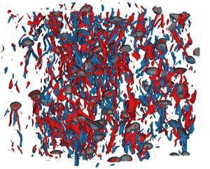
The plots in figures 1(a) and 1(b) show a representative snapshot of bubbles and iso-vorticity surfaces for $\textit {Re}_{\lambda }=79,b=0.35$ and $\textit {Re}_{\lambda }=110,b=0.13$, respectively. In figure 1(c,d) we show a few typical trajectories for the same parameters. It is clear that higher Reynolds number and small ‘bubblance’ parameter correspond to more complex trajectories. To quantify this behaviour, we plot the p.d.f. of the curvature ${\mathcal {K}}\equiv {\mid {\boldsymbol {A}} \times {\boldsymbol {V}}\mid /\mid {\boldsymbol {V}}\mid ^3}$ in figure 1(e). Consistent with the observation that the trajectories are more curved for larger $\textit {Re}_{\lambda }$, we find that the p.d.f. $P({\mathcal {K}})$ is broader – has an exponential tail.

Figure 1. Representative steady-state snapshot of the bubbles and superimposed iso-surfaces of the $z$ component of the vorticity field 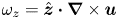$\omega _z=\hat {\boldsymbol {z}} \boldsymbol {\cdot } \boldsymbol {\nabla } \times \boldsymbol {u}$ for $\omega _z=\pm 3\left \langle \omega _z^2\right \rangle ^{1/2}$ for (a) $b=0.35$ and (b) $b=0.13$. Typical trajectories of the centre of mass of bubbles in a turbulent flow for (c) $\textit {Re}_{\lambda }=79$, $b=0.35\ ({\texttt {R1}})$ and (d) $\textit {Re}_{\lambda }=110$, $b=0.13\ ({\texttt {R3}})$. (e) The p.d.f. of the curvature ${\mathcal {K}}$ for different values of $b$. (f) Plot showing that the bubble rise velocity increases with increasing $b$ or decreasing $\textit {Re}_{\lambda }$. We also show that $U$ obtained directly from the trajectories and the estimate $\varepsilon ^{g}/(2 \textit {At} g \varPhi )$ are in excellent agreement.

Note that Bhatnagar et al. (Reference Bhatnagar, Gupta, Mitra, Perlekar, Wilkinson and Pandit2016) showed that the p.d.f. of curvature of trajectories of heavy inertial particles in homogeneous and isotropic turbulence has a power-law tail with an exponent of $-5/2$. To the best of our knowledge, no such results exist for bubbles.

Another consequence of large-scale turbulent stirring is that the average bubble rise velocity $U \equiv (1/N_b) \sum _{{i}=1}^{N_b} \overline {\boldsymbol {V}_{i}(t)\boldsymbol {\cdot } {\hat {\boldsymbol {z}}}}$ (see figure 1f) increases with increasing $b$ (decreasing $\textit {Re}_{\lambda }$), where $\overline {(\boldsymbol {\cdot })}$ represents temporal averaging.

In a recent study, Salibindla et al. (Reference Salibindla, Masuk, Tan and Ni2020) showed that the rise velocity of the bubbles can be enhanced by turbulence provided the velocity ratio $\gamma \equiv (V_0^2/(\varepsilon ^{s} d)^{2/3})<1$. Our DNS (see table 2) and the experiments that investigate turbulence modulation by bubbles (Lance & Bataille Reference Lance and Bataille1991; Prakash et al. Reference Prakash, Mercado, van Wijngaarden, Mancilla, Tagawa, Lohse and Sun2016) have $\gamma \gg 1$.

Table 2. Velocity ratio $\gamma$ for our DNS runs ${\texttt {R1}}$–${\texttt {R3}}$.

Note that even for $b=\infty$, the rise velocity of a bubble in a swarm is slightly smaller than the rise velocity of an isolated bubble due to bubble–wake interactions (Riboux, Risso & Legendre Reference Riboux, Risso and Legendre2010). Using the definition of $\boldsymbol {F}^{g}$ and noting that $\left \langle u_z\right \rangle =0$ in the Boussinesq regime, we obtain $\varepsilon ^{g}= 2\textit {At} g \varPhi U$ and verify it in figure 1(f).

3.2. Pair distribution function

To understand the distribution of bubbles in the domain, following Bunner & Tryggvason (Reference Bunner and Tryggvason2002a), we define the pair distribution function:

(3.1)\begin{equation} G[r,\cos(\theta)] = \frac{L^3}{N_{b}(N_{b}-1)}\overline{{\sum_{{i}=1}^{N_{b}}\sum_{{j}=1, {j} \ne {i}}^{N_{b}} \delta({\boldsymbol{r}} - {\boldsymbol{X}}_{{ij}},t)}}, \end{equation}

where $\delta (\boldsymbol {\cdot })$ is the Dirac delta function and ${\boldsymbol{X}}_{{ij}}={\boldsymbol{X}}_{i}-{\boldsymbol{X}}_{j}$. In figure 2(a), we sketch a bubble pair configuration to show the coordinate system used for evaluating (3.1). Plots of $G[r,\cos (\theta )]$ for $r=2d$ and $4d$ are shown in figure 2(b). At $b=\infty$, we observe a peak in $G[r,\cos (\theta )]$ for $r \approx 2d$ and $\cos (\theta )\approx 0$ indicating a horizontal alignment of bubbles that are separated by a distance $2d$. Bubbles separated by distances $r\geqslant d$ are uniformly distributed. Our results are consistent with earlier numerical studies of pseudo-turbulence (Bunner & Tryggvason Reference Bunner and Tryggvason2002a; Roghair, Annaland & Kuipers Reference Roghair, Annaland and Kuipers2013). In contrast, as turbulence makes flow more isotropic, for $b=0.13$ we find that $G[r,\cos (\theta )]$ is uniform which indicates that the bubbles are uniformly distributed for all separations $r$.

Figure 2. (a) The separation vector ${\boldsymbol {r}}= {\boldsymbol {X}}_{i}-{\boldsymbol {X}}_{j}$ and the angle $\theta$ between ${\boldsymbol {X}}_{ij}$ and $\hat {\boldsymbol {z}}$. The bubbles are represented as shaded ellipses. (b) The angular distribution function $G[r,\cos (\theta )]$ versus $\cos (\theta )$ for $r=2d$ and $r=4d$ in the absence ($b=\infty$) and presence ($b=0.13$) of turbulence. The area under the curve is normalized to unity for each $G[r,\cos (\theta )]$ curve.

3.3. Average flow around a bubble

In this section, we study the average wake structure of the bubbles for different values of bubblance $b$. At a given time $t$, the velocity field in the centre-of-mass frame of the bubble ${i}$ is given by

(3.2)\begin{equation} {\boldsymbol{u}}^{CM}_{i}({\boldsymbol{\xi}},t)= \boldsymbol{u}({\boldsymbol{\xi}},t)- {\boldsymbol{V}}_{i}, \end{equation}

where ${\boldsymbol {\xi }}\equiv {\boldsymbol {x}}-{\boldsymbol{X}}_{i}$ and $-L/2 < (\xi _x,\xi _y,\xi _z) \leqslant L/2$. The average flow around a bubble is then obtained by performing temporal averaging over every bubble as follows:

(3.3)\begin{equation} {\boldsymbol{u}}^{CM}({\boldsymbol{\xi}}) = \frac{1}{N_{b}}\sum^{N_{b}}_{{i}=1} \overline{{\boldsymbol{u}}^{CM}_{i}({\boldsymbol{\xi}},t)}. \end{equation}

In figure 3(a,b) we plot the velocity streamlines of the average velocity field ${\boldsymbol {u}}^{CM}({\boldsymbol {\xi }})$ for $b=\infty$ (${\texttt {R0}}$) and $b=0.13$ (${\texttt {R3}}$). Although the flow structures look qualitatively similar, we find that the bubble in the absence of large-scale stirring is more ellipsoidal. This can be understood by noting that the presence of stirring imposes stronger isotropy on the flow.

Figure 3. Streamline plots of the average velocity field in the frame of the bubble for (a) $b=\infty$ (run ${\texttt {R0}}$) and (b) $b=0.13$ (run ${\texttt {R3}}$). The streamlines are coloured according to $\boldsymbol {u}^{CM}\boldsymbol {\cdot }\hat {\boldsymbol {z}}$.

To quantify the behaviour of the average bubble wake, similar to experiments (Risso et al. Reference Risso, Roig, Amoura, Riboux and Billet2008; Almeras et al. Reference Almeras, Mathai, Lohse and Sun2017) we plot $v(\xi _z)\equiv \boldsymbol {u}^{CM}(0,0,\xi _z)\boldsymbol {\cdot }\hat {\boldsymbol {z}}$ in figure 4 and find that it decays exponentially as $v(\xi _z)\sim C \exp (-A \xi _z/d)$ in the wake region for all values of $b$. However, consistent with earlier observations, the presence of stirring leads to a faster decay of the wake. Therefore, for small $b$ (or large $\textit {Re}_{\lambda }$) we expect (see next section) the velocity fluctuations to be similar to those of homogeneous, isotropic turbulence.

Figure 4. (a) The average bubble wake velocity $v(\xi _z)$ for runs ${\texttt {R0}}$ ($b=\infty$), ${\texttt {R1}}$ ($b=0.35$) and ${\texttt {R3}}$ ($b=0.13$). (b) Same as (a), but in semi-log scale to highlight the exponential decay of the velocity field in the wake region. The dash-dotted lines show the exponential fits 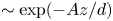$\sim \exp (-A z/d)$ to the data. We find $A=0.67$, $1.15$ and $1.6$ for ${\texttt {R0}}$, ${\texttt {R1}}$ and ${\texttt {R3}}$, respectively.

3.4. Liquid velocity fluctuations

The p.d.f.s of the normalized horizontal and vertical liquid velocity fluctuation with varying $b$ are shown in figure 5. For $b=\infty$, our results agree with those of the earlier studies on pseudo-turbulence (Riboux et al. Reference Riboux, Risso and Legendre2010; Risso Reference Risso2016; Pandey et al. Reference Pandey, Ramadugu and Perlekar2020): the p.d.f. of the horizontal component shows exponential behaviour and the p.d.f. of the vertical component has a Gaussian core and is positively skewed. The presence of external stirring dramatically alters the p.d.f.s as they tend to a Gaussian distribution with decreasing $b$ (increasing $\textit {Re}_{\lambda }$). Indeed, in the inset of figure 5(a), we verify that $\langle u_h^2 \rangle \sim \langle u_z^2 \rangle$ on decreasing $b$ confirming that the stirring makes the flow isotropic. This is consistent with earlier experimental observations of turbulent bubbly flows (Prakash et al. Reference Prakash, Mercado, van Wijngaarden, Mancilla, Tagawa, Lohse and Sun2016; Almeras et al. Reference Almeras, Mathai, Lohse and Sun2017).

Figure 5. The p.d.f. of the horizontal (a) and the vertical (b) component of the liquid velocity fluctuations for different values of $b$ (blue, $b=\infty$ (${\texttt {R0}}$); orange, $b=0.35$ (${\texttt {R1}}$); green, $b=0.21$ (${\texttt {R2}}$); maroon, $b=0.13$ (${\texttt {R3}}$); purple, $b=0$ ($\textit {Re}_{\lambda }=110$)). The black dashed line indicates a Gaussian distribution, and the brown dash-dotted line in (a) shows the exponential distribution. Inset: variance of the horizontal and vertical velocity fluctuations increases with an increase in the stirring intensity $1/b$.

3.5. Energy spectrum

Earlier DNS studies (Roghair et al. Reference Roghair, Mercado, Annaland, Kuipers, Sun and Lohse2011; Pandey et al. Reference Pandey, Ramadugu and Perlekar2020; Innocenti et al. Reference Innocenti, Jaccod, Popinet and Chibbaro2021) only investigated the nature of the energy spectrum in the absence of large-scale turbulent forcing. These studies, consistent with experiments, confirm the presence of a $k^{-3}$ scaling in the spectrum that appears because of the balance of net energy production in the wakes with viscous dissipation.

Experiments have investigated temporal spectra of the Eulerian liquid velocity fluctuations in the presence of a large-scale stirring. They observe a Kolmogorov spectrum for frequencies smaller than the bubble frequency and a pseudo-turbulence scaling for higher frequencies (Lance & Bataille Reference Lance and Bataille1991; Prakash et al. Reference Prakash, Mercado, van Wijngaarden, Mancilla, Tagawa, Lohse and Sun2016; Almeras et al. Reference Almeras, Mathai, Lohse and Sun2017).

Hence we expect that in our simulations we would find a Kolmogorov scaling for wavenumbers $k< k_{d}$, with a crossover to pseudo-turbulence scaling for $k>k_{d}$, where $k_{d}\equiv 2{\rm \pi} /d$ is the wavenumber corresponding to the bubble diameter.

In figure 6, we plot the scaled energy spectrum for different values of $b$ ($\textit {Re}_{\lambda }$). As expected, we observe Kolmogorov scaling 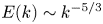$E(k)\sim k^{-5/3}$ for $k< k_{d}$ and a pseudo-turbulence scaling $E(k) \sim k^{-3}$ for $k>k_{d}$. In figure 7 we plot the compensated spectrum to highlight the region showing $-5/3$ and $-3$ scaling. Note that none of the scaling ranges are large enough to make possible an accurate determination of the scaling exponent.

Figure 6. Log–log plot of the kinetic energy spectrum $E(k)$ versus $k/k_{d}$ for (a) $b=0.35,\textit {Re}_{\lambda }=79$ (${\texttt {R1}}$) and (b) $b=0.13,\textit {Re}_{\lambda }=110$ (${\texttt {R3}}$).

Figure 7. Compensated plot of the kinetic energy spectrum highlighting the (a) $-5/3$ and (b) $-3$ scaling ranges. Horizontal dashed line and the shaded region indicate the scaling range.

3.6. Scale-by-scale energy budget and flux

To lay bare the mechanism by which bubbly turbulence emerges we study the scale-by-scale energy budget. Following Pope (Reference Pope2012) we define a low-pass-filtered velocity field coarse-grained at scale $\ell =2{\rm \pi} /K$ as

(3.4)\begin{equation} \boldsymbol{u}^{<}_{K}(\boldsymbol{x}) \equiv \int\exp(\textrm{i}\boldsymbol{q}\boldsymbol{\cdot}\boldsymbol{x}) G_{K}(\boldsymbol{q})\hat{\boldsymbol{u}}(\boldsymbol{q})\,\textrm{d}\boldsymbol{q} ,\quad \textrm{with} \ G_{K}(\boldsymbol{q}) \equiv \exp\left(-\frac{{\rm \pi}^2q^2}{24 K^2}\right) . \end{equation}

Note that Frisch (Reference Frisch1997) and Pandey et al. (Reference Pandey, Ramadugu and Perlekar2020) use a sharp stepdown function as a filter: $G_{K}(\boldsymbol {q}) = 1$ for $\mid \boldsymbol {q}\mid \leqslant K$ and zero otherwise. In contrast, we use a smooth Gaussian filter (Pope Reference Pope2012). In what follows, we use the symbol $\left (\boldsymbol {\cdot }\right )^{<}_{ K}$ to denote the filtering operation (Frisch Reference Frisch1997). In real space, this corresponds to

(3.5)\begin{align} \boldsymbol{u}^{<}_{K}(\boldsymbol{x}) \!=\! \int G_\ell({\boldsymbol{r}})\boldsymbol{u}(\boldsymbol{x} - {\boldsymbol{r}})\,\textrm{d}{\boldsymbol{r}},\quad \textrm{with}\ G_\ell({\boldsymbol{r}})\!=\! \left(\frac{6}{{\rm \pi}\ell^2}\right)^{1/2}\exp\left(-\frac{6r^2}{\ell^2}\right)\quad \textrm{{and}}\quad \ell \equiv\! 2{\rm \pi}/K. \end{align}

Using the filtered velocity field, we obtain the following scale-by-scale energy budget equation from (2.1a,b):

(3.6)\begin{equation} \varPi_K + {\mathscr{F}}^{\sigma}_{K} ={-} {\mathscr{D}}_{K} + {\mathscr{F}}^{g}_{K} + {\mathscr{F}}^{s}_{K}.\end{equation}

Here 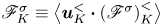${\mathscr {F}}^{\sigma }_{K} \equiv \left \langle \boldsymbol {u}^{<}_{K} \boldsymbol {\cdot } \left (\mathscr {F}^{\sigma }\right )_{K}^{<}\right \rangle$ is the contribution from surface tension forces, 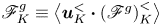${\mathscr {F}}^{g}_{K} \equiv \left \langle {\boldsymbol {u}^{<}_{K} \boldsymbol {\cdot } \left (\mathscr {F}^{g}\right )_{K}^{<}}\right \rangle$ is the contribution from buoyancy and 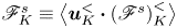${\mathscr {F}}^{s}_{K} \equiv \left \langle {\boldsymbol {u}_K^{<}\boldsymbol {\cdot } \left (\mathscr {F}^{s}\right )_K^{<}}\right \rangle$ is the contribution due to large-scale forcing. To obtain the contribution from the nonlinear term and viscous dissipation, following Eyink (Reference Eyink1995), Borue & Orszag (Reference Borue and Orszag1998) and Pope (Reference Pope2012), we define a filtered version of the Reynolds stress tensor

(3.7)\begin{equation} \boldsymbol{\mathsf{T}}^{\alpha\beta}_{ K}({\boldsymbol{x}}) \equiv \left(u^{\alpha}u^{\beta}\right)^{<}_{K} - \left(u^{\alpha}\right)^{<}_{K}\left(u^{\beta}\right)^{<}_{K}, \end{equation}

the rate-of-strain tensor

(3.8)\begin{equation} \boldsymbol{\mathsf{S}}_{K}^{\alpha\beta}({\boldsymbol{x}}) \equiv \tfrac{1}{2}\left[\left(\partial_{\alpha}u^{\beta}\right)^{<}_{K}+\left(\partial_{\beta}u^{\alpha}\right)^{<}_{K} \right] \end{equation}

and the local nonlinear energy flux

(3.9)\begin{equation} {\rm \pi}_{K}({\boldsymbol{x}}) \equiv{-}\boldsymbol{\mathsf{T}}^{\alpha\beta}_{ K}\boldsymbol{\mathsf{S}}_{K}^{\alpha\beta} . \end{equation}

Using (3.4), (3.7), (3.8) and (3.9), we get the net nonlinear flux $\varPi _{K} \equiv \left \langle {\rm \pi}_{K}\right \rangle$, and the viscous contribution to the budget ${\mathscr {D}}_{K} \equiv 2\nu \left \langle {\boldsymbol{\mathsf{S}}_{K}^{\alpha \beta }\boldsymbol{\mathsf{S}}_{K}^{\alpha \beta }}\right \rangle$ which is always positive.

3.6.1. Scale-by-scale energy budget in the absence of bubbles ($b=0$)

In this case buoyancy makes no contribution to the fluxes and (3.6) simplifies to

(3.10)\begin{equation} \varPi_K ={-} {\mathscr{D}}_{K} + {\mathscr{F}}^{s}_{K} . \end{equation}

The plot in figure 8(a) shows the energy budget for $b=0$ ($\textit {Re}_{\lambda }=110$). Since the stirring force is limited to small Fourier modes $k\leqslant k_{inj}$, ${\mathscr {F}}^{s}_{K}=\varepsilon ^{s}$ is a constant for $K>k_{inj}$. The viscous contribution ${\mathscr {D}}_{K}$ is significant only for very large $K \geqslant k_{\eta }$. Hence, for intermediate values of $K$ in the inertial range ($k_{inj} < K < k_{\eta }$), the flux $\varPi _{K} = {\mathscr {F}}^{s}_{K}$ remains a constant. The four-fifths law of Kolmogorov and the Kolmogorov scaling, $E(k) \sim k^{-5/3}$, are a consequence of this constancy of flux (e.g. Frisch Reference Frisch1997, § 6.2). Because of the moderate $\textit {Re}_{\lambda }=110$ used by us, the range of wavenumbers over which the flux is constant is very small. A significant range of constant flux is observed in very-high-$\textit {Re}_{\lambda }$ and large-resolution DNS (Ishihara, Gotoh & Kaneda Reference Ishihara, Gotoh and Kaneda2009).

Figure 8. Scale-by-scale energy budget: plot of the energy flux $\varPi _K$, cumulative viscous dissipation ${\mathscr {D}}_{K}$, the surface tension contribution ${\mathscr {F}}^{\sigma }_{K}$, the cumulative energy injected due to buoyancy ${\mathscr {F}}^{g}_{K}$ and the energy injected due to turbulent forcing ${\mathscr {F}}^{s}_{K}$ for $b=0\ (\textit {Re}_{\lambda } = 110)$ (a), $b=\infty$ (b), $b=0.35$ (c) and $b=0.13$ (d). The black dashed line indicates $\log ({K})$ scaling. In (a–d) we normalize the ordinate by the viscous dissipation $\varepsilon ^{\nu }$. In (a,c,d) we mark the injection wavenumbers by a shaded region.

3.6.2. Scale-by-scale budget in the absence of stirring ($b=\infty$)

Next, in figure 8(b) we study the other extreme, $b=\infty$. Stirring makes no contribution here. Energy injection by buoyancy forces happens around the scale of the bubble diameters and the flux due to buoyancy ${\mathscr {F}}^{g}_{K}$ becomes almost a constant for $K \gg k_{d}$. Hence for $K \gg k_{d}$ we obtain

(3.11)\begin{equation} \varPi_{K} + {\mathscr{F}}^{\sigma}_{K} ={-} {\mathscr{D}}_{K} + {\mathscr{F}}^{g}_{K} , \end{equation}

with ${\mathscr {F}}^{g}_{K}$ approximately a constant. By taking a derivative of both sides of (3.11) with respect to $K$ at $K = k$ we obtain

(3.12)\begin{equation} \left.\frac{\textrm{d}(\varPi_{K}+{\mathscr{F}}^{\sigma}_{K})}{\textrm{d}K}\right\rvert_{K=k} = \nu k^2E(k). \end{equation}

Our DNS shows that the net production $\varPi _{K}+{\mathscr {F}}^{\sigma }_{K} \sim \log (K)$ (Lance & Bataille Reference Lance and Bataille1991; Pandey et al. Reference Pandey, Ramadugu and Perlekar2020). Although taking a derivative can enhance approximation errors, we directly confirm the scaling relation in figure 9. Generalizing the argument of Lance & Bataille (Reference Lance and Bataille1991), if we now assume locality of net transfer then by dimensional analysis $\textrm {d}(\varPi _K + {\mathscr {F}}^{\sigma }_{K})/\textrm {d} K\mid _{K=k} \sim k^{-1}$ follows. Substituting in (3.12) we obtain $E(k) \sim k^{-3}$ – the spectrum of pseudo-turbulence (Lance & Bataille Reference Lance and Bataille1991; Mercado et al. Reference Mercado, Gomez, Gils, Sun and Lohse2010; Prakash et al. Reference Prakash, Mercado, van Wijngaarden, Mancilla, Tagawa, Lohse and Sun2016; Almeras et al. Reference Almeras, Mathai, Lohse and Sun2017; Bunner & Tryggvason Reference Bunner and Tryggvason2002b; Roghair et al. Reference Roghair, Mercado, Annaland, Kuipers, Sun and Lohse2011; Pandey et al. Reference Pandey, Ramadugu and Perlekar2020; Ramadugu et al. Reference Ramadugu, Pandey and Perlekar2020). Risso (Reference Risso2011) has shown that the same $k^{-3}$ spectrum can be obtained, under certain conditions, as a sum of localized random, statistically independent, bursts, which comes from localized velocity disturbances caused by the bubbles.

Figure 9. Log–log plot of $(K/k_d) |\,\textrm {d}({\mathscr {F}}^{\sigma }_{K} + \varPi _K)/\textrm {d}K|$ versus $K/k_d$ for different values of the bubblance parameter $b$. Horizontal dashed lines represent $K^{-1}$ scaling.

3.6.4. Spatial distribution of the nonlinear energy flux ${\rm \pi} _{K}(x)$

For homogeneous and isotropic turbulence, for any $K$ in the inertial range, the net nonlinear flux $\varPi _{K}$ is positive, i.e. on average energy flows from small to large $K$ or from large to small spatial scales. Kraichnan (Reference Kraichnan1974) and Eyink (Reference Eyink1995) argued that the local nonlinear energy flux ${\rm \pi} _{K}$ (3.9) satisfies the refined similarity hypothesis. Using DNS, Chen et al. (Reference Chen, Chen, Eyink and Holm2003) verified this and showed that the scaling exponents of the flux show multiscaling. The multiscale analysis of the flux is also crucial to model subgrid-scale dissipation in large-eddy simulations (Meneveau & Katz Reference Meneveau and Katz2000).

To the best of our knowledge, the spatial distribution of local energy flux in bubbly flows remains unexplored. How does the sign of this flux correlate with the bubbles? For example, is the flux predominantly positive in the wake of a bubble? In the following discussion, we address this question by performing a multiscale analysis of the local nonlinear energy flux ${\rm \pi} _{K}(\boldsymbol {x})$ with varying filtering scale $\ell \sim 1/K$.

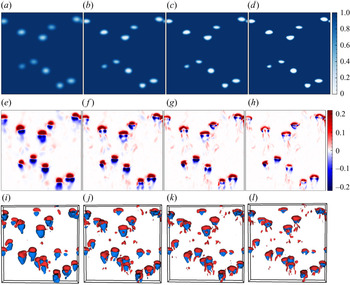
In figure 10, we show a typical snapshot from the run with no external stirring, $b=\infty$. The position of the bubbles is shown by plotting the indicator function in figure 10(a–d). In figure 10(e–l), we plot the local nonlinear flux ${\rm \pi} _{K}$. In each panel, we use four different values for the filtering wavenumber $K/k_{d} = 0.6$, 1.0, $1.4$ and $2.2$, from left to right. Note that we use a Gaussian filter; therefore, a proper distinction between liquid and bubble phase can be made only for $K>k_{d}$. We make the following observations:

1. (i) In the front of the bubble, the energy is primarily transferred downscale, i.e. to scales smaller than $\ell \sim 1/K$.

2. (ii) Depending on the filtering scale, we observe both upscale and downscale transfer of energy in the wake of the bubble. For large $K$ (small $\ell$), downscale transfer of energy dominates the wake region, but there are also regions of upscale transfer.

3. (iii) On reducing the filter wavenumber $K$ (large $\ell$), we observe that the region of upscale transfer is enhanced in the rear region of the bubble. For the smallest filtering wavenumber $K/k_{d}=0.6$, the front–rear region of the bubble has a similar structure but appears with opposite signs.

Figure 10. Buoyancy-driven flow in the absence of stirring ($b=\infty$, ${\texttt {R0}}$). The pseudo-colour plot of the filtered indicator function $c$ (a–d) and the local nonlinear flux ${\rm \pi} _{K}/\max ({\rm \pi} _{k_{d}})$ (e–h) in the $y=L/2$ plane. Constant-${\rm \pi} _{K}$ iso-surfaces for $|{\rm \pi} _{K}|=0.03 \max ({\rm \pi} _{k_{d}})$ in a slab $L \times 2d \times L$ around the $y=L/2$ plane (i–l). The filter wavenumber (scale) is increased (decreased) from left to right: $K/k_{d}=0.6$, 1.0, $1.4$ and $2.2$.

We can understand the fore–aft structure of the energy flux in the vicinity of a bubble in a straightforward manner. Consider a Stokesian spherical bubble with the same viscosity as ambient fluid rising in a quiescent flow; the stream function is given by the Hadamard–Rybczynski solution (Hadamard Reference Hadamard1911; Rybczynski Reference Rybczynski1911; Clift, Grace & Weber Reference Clift, Grace and Weber1978):

(3.13)\begin{equation} \varPsi(r,\theta) = \frac{V_0 r^2 \sin^2(\theta)}{2} \begin{cases} -\left(1 - \dfrac{5 d}{8r} + \dfrac{d^3}{32 r^3} \right) & \text{for}\ r\geqslant d/2,\\ \dfrac{1}{4}\left(1 - \dfrac{4 r^2}{d^2} \right) & \text{for}\ r< d/2. \end{cases} \end{equation}

The radial and angular components of the velocity field are $u_r=\partial _\theta \varPsi /r^2 \sin (\theta )$ and 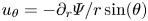$u_\theta =-\partial _r \varPsi /r \sin (\theta )$. Using (3.13), we calculate the nonlinear flux ${\rm \pi} _{K}$ and plot it in figure 11 for four different values of the filtering wavenumber $K/k_{d} = 0.6$, 1.0, 1.4 and $2.2$. There is a downscale energy transfer in the front and an upscale energy transfer at the back side of the bubble. Note that the net energy flux $\varPi _{K}$ is zero for the Hadamard–Rybczynski solution. Comparing figure 10 with figure 11, it seems that the spatial distribution of the energy flux comprises a Hadamard–Rybczynski-like solution superimposed with turbulent fluctuations generated in the wake region of a rising bubble. Thus our multiscale analysis of the spatial energy flux provides direct evidence that the net forward energy flux in figure 8(b) is due to the bubble wakes.

Figure 11. The space-dependent nonlinear flux ${\rm \pi} _{K}/\max ({\rm \pi} _{k_{d}})$ in the $y=L/2$ plane for the Hadamard–Rybczynski flow (3.13). The filter wavenumber (scale) is increased (decreased) from left to right: $K/k_{d}=$ (a) $0.6$, (b) 1.0, (c) 1.4 and (d) $2.2$. The green line represents the bubble interface.

The situation is more complex in the presence of stirring, as now both the large-scale forcing as well as the wake of the bubble creates complex spatio-temporal patterns for ${\rm \pi} _{K}(\boldsymbol {x})$ with regions of downscale and upscale transfer (see figure 12). In figure 13 we plot the p.d.f. of ${\rm \pi} _{K}(\boldsymbol {x})$ with $K=k_{d}$ for $b=0$, $b=0.13$ and $b=\infty$. For all the cases we observe that the p.d.f. is positively skewed confirming a net positive flux of energy. The skewness of the p.d.f. for $b=0$ is nearly $1.3$ times larger than that for $b=\infty$, indicating the presence of stronger inverse energy transfers in buoyancy-driven bubbly flows in comparison with homogeneous, isotropic turbulence. This is further verified by noting that the skewness for $b=0.13$, where both stirring and buoyancy-driven bubbles generate turbulence, is smaller than the case with $b=0$.

Figure 12. Buoyancy-driven flow in presence of stirring ($b=0.13$, ${\texttt {R3}}$). The pseudo-colour plot of the filtered indicator function $c$ (a–d) and the local nonlinear flux ${\rm \pi} _{K}/\max ({\rm \pi} _{k_{d}})$ (e–h) in the $y=L/2$ plane. Constant-${\rm \pi} _{K}$ iso-surfaces for $|{\rm \pi} _{K}|=0.03 \max ({\rm \pi} _{k_{d}})$ in a slab $L\times 2d\times L$ around the $y=L/2$ plane (i–l). The filter wavenumber (scale) is increased (decreased) from left to right: $K/k_{d}=0.6$, 1.0, 1.4 and $2.2$.

Figure 13. The p.d.f. of the scaled nonlinear flux ${\rm \pi} _{K}/\langle {\rm \pi}_{K}^2\rangle ^{1/2}$ for different values of $b$, and with $K=k_{d}$.

3.7. Total energy budget

Using (2.1a,b) we obtain the steady-state total energy budget equation as

(3.14)\begin{equation} \varepsilon^{g}+\varepsilon^{s}=\varepsilon^{\nu}, \end{equation}

i.e. energy injected by buoyancy and stirring is dissipated by viscosity. Using table 1, (3.14) is easily verified.

In this section, we study the contribution to the total budget from each of the phases. The two phases are characterized by the indicator function $c$ which takes value $1$ in the liquid phase, $0$ inside the bubble and an intermediate value at the interface. In a DNS of two-phase flows, usually the interface is diffused over 3–4 grid points. Thus, using $c$ to distinguish the phases implies that the interface region contributes to both the phases. In order to avoid this conundrum, we construct a new indicator function $c^{\prime }$ such that the interface points are included inside the bubble. To construct $c^\prime$ we first initialize it to be the same as $c$. The points that lie closest to $c^\prime =1/2$ contour are identified as bubble interface points. For points where $c^\prime <1/2$, $c^\prime$ is set to zero and it is unity outside. Next we set $c^\prime =0$ at all points that are within a distance of $0.16d$ from the interface points. This completes the procedure of generating an inflated region around each bubble.

Henceforth we use the term bubble to indicate the regions where $c^{\prime }=0$. Using $c^{\prime }$ we define the net injection and dissipation rates in the liquid as

(3.15a)\begin{gather} \varepsilon^{\nu}_{l} = 2 \nu\left\langle c^{\prime} \boldsymbol{\mathsf{S}} : \boldsymbol{\mathsf{S}} \right\rangle, \end{gather}

(3.15b)\begin{gather}\varepsilon^{g}_{l} = \left\langle c^{\prime}\boldsymbol{u} \boldsymbol{\cdot} \boldsymbol{F}^{g} \right\rangle, \end{gather}

(3.15c)\begin{gather}\varepsilon^{s}_{l} =\left\langle c^{\prime}\boldsymbol{u} \boldsymbol{\cdot} \boldsymbol{F}^{s} \right\rangle. \end{gather}

The contribution from the bubble phase can be obtained by subtracting the contribution from the liquid phase from the total. For instance, dissipation rate in the bubble phase is $\varepsilon ^{\nu }_{b} = \varepsilon ^{\nu } - \varepsilon ^{\nu }_{l}$.

In figure 14(a,b) we show the pseudo-colour plot of the local viscous dissipation 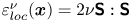$\varepsilon ^{\nu }_{loc}(\boldsymbol {x})=2 \nu \boldsymbol{\mathsf{S}}:\boldsymbol{\mathsf{S}}$. For the case with no stirring, $b=\infty$, the dissipation is strongly concentrated inside and in the wake of the bubbles, whereas when stirring is present, $b=0.13$, strong dissipation is also observed in the liquid phase away from the bubbles.

Figure 14. Pseudo-colour plot of the local dissipation $\varepsilon ^{\nu }_{loc}$ in $y=L/2$ plane for (a) $b=\infty$ (run ${\texttt {R0}}$) and (b) $b=0.13$ (run ${\texttt {R3}}$). The black line represents the bubble interface ($c=0$ contour) and the blue line indicates the contour $c'=0$.

In figure 15(a) we look at the balance between energy injection and dissipation in each phase for the case of no stirring, $b=\infty$. In the liquid phase, viscous dissipation $\varepsilon ^{\nu }_{l}$ far exceeds energy injected due to buoyancy $\varepsilon ^{g}_{l}$, whereas in the bubble phase the situation is reversed. Note that the overall viscous dissipation inside the bubble phase is larger than the overall dissipation in the liquid phase.

Figure 15. The dissipation and injection rates in the steady state evaluated in the liquid and bubble phases for (a) $b=\infty$ (run ${\texttt {R0}}$) and (b) $b=0.13$ (run ${\texttt {R3}}$). The ordinate in both panels is normalized by $\varepsilon ^{\nu }$.

We can now summarize the flow of energy completely for the case of no stirring, $b=\infty$. Buoyancy force injects energy at the scale of the bubbles, largely in the gas phase. A large fraction of this energy is dissipated within the bubble itself. The rest of it is transferred to the liquid phase by bubble–liquid interaction. Both the nonlinear flux and the flux due to the surface tension cascade this energy to smaller and smaller scales in the fluid. Energy dissipation happens in both the gas and liquid phases starting from the scale of the bubble down to the smallest scales.

We next plot the injection and dissipation rates obtained for different phases for the case $b=0.13$ in figure 15(b). Here, we find that dominant energy injection is due to the stirring. This appears largely in the liquid phase. The net energy dissipated in the liquid phase exceeds the energy injected by stirring due to the additional energy transfer from the bubble phase to the liquid phase. In the bubble phase, energy is injected by the buoyancy forces. Most of this energy is dissipated in the bubble phase, but as pointed out above, a part of it is also transferred to the liquid phase.