2.1.1 Analysis using Keras

In this section, we show how Keras can be used to fit several variations of the shallow neural network discussed in Noll et al. (Reference Noll, Salzmann and Wüthrich2018). At the outset, it is worth noting that the signal-to-noise ratio of claims frequency data is often relatively low (see Section 2.5.5 in Wüthrich and Buser (Reference Wüthrich and Buser2018)) and very flexible or high-dimensional models might not provide much extra accuracy with this type of data.

As noted above, neural networks learn representations of the features that are optimal for the problem they are optimised on, by stacking layers of neurons on top of each other. Each hidden layer can be thought of as a non-linear regression with a feature representation as the output. A neural network without any hidden layers (i.e. without representation learning) is simply equivalent to a regression model, and, therefore, for ease of exposition, we start with a GLM model in Keras, following the data processing steps in Noll et al. (Reference Noll, Salzmann and Wüthrich2018). As mentioned above, after noticing that the assumption of linearity was violated for some of the continuous feature variables, Noll et al. (Reference Noll, Salzmann and Wüthrich2018) apply some feature engineering by discretising these variables (for details, see the code accompanying that paper), thus, the GLM mentioned in this section allows for some non-linear relationships. A different approach would be to use a GAM, which relies on splines to model non-linear relationships between the features and the output ^{Footnote 3} .

Two points should be noted when trying to use Keras to fit a Poisson rate regression. Firstly, Keras includes a Poisson loss function, the minimisation of which is equivalent to minimising the Poisson Deviance; nonetheless, the values returned by this function are not equal to the Poisson Deviance. If the user wishes to track the Poisson Deviance during training, then this may be remedied by defining a custom Poisson Deviance loss function. Secondly, the model required is a Poisson rate regression, where the exposure measure is the time that a policy is in force, and the regression fits the rate of claim based on this exposure measure. To fit this model in Keras, the easiest option is to use the Keras Functional Application Programming Interface (API) to multiply the output of the neural network with the exposure to derive the expected number of claims. Since the rates of claim lie between 0 and 1, the output layer of the neural network was chosen to use a sigmoid activation, and therefore, the network learns the rates on a logit scale, which is slightly different from the log scale used by the GLM. This model is denoted GLM_Keras in Table 1, whereas the baseline GLM fit using the glm() function in R is denoted GLM. The code in R to accomplish this is

Table 1. Out-of-sample Poisson deviance for the French TPL dataset

\begin{equation*} \textit{dense}=\textit{NumInputs}\ \%{>}\% \end{equation*}

\begin{equation*} \textit{layer\_dense(units}=\textit{1}, \textit{activation} = \textit{``sigmoid'')} \end{equation*}

\begin{equation*} \textit{N} = \textit{layer\_multiply(list(dense,Exposure), name} = \textit{``N'')} \end{equation*}

The out-of-sample Poisson deviance in Table 1 for the GLM fit in Keras is close to that of the baseline GLM. Fitting a shallow neural network requires a single extra line of code:

\begin{equation*} \textit{dense}=\textit{NumInputs}\ \%{>}\% \end{equation*}

\begin{equation*} \textit{layer\_dense(units}=\textit{20}, \textit{activation} = \textit{``relu'')}\ \%{>}\% \end{equation*}

\begin{equation*} \textit{layer\_dense(units}=\textit{1}, \textit{activation} = \textit{``sigmoid'')} \end{equation*}

In this case, a hidden layer with 20 neurons was used, with the ReLu activation function. The same dataset used for the GLM that contained the categorical conversion of the numerical inputs was used as the data in this network, which performed on a par with the neural network model in Noll et al. (Reference Noll, Salzmann and Wüthrich2018) and is denoted NN_shallow in the table. However, this model is somewhat unsatisfying since it relies on manual feature engineering, that is, converting the numerical inputs to categorical values.

Therefore, another network (denoted NN_no_FE) was tried, but the out-of-sample performance was worse than the GLM, indicating that the network did not manage to fit continuous functions to the numerical inputs properly. To overcome this deficiency, the specialised embedding layer discussed above was added to the model for all of the numerical and categorical variables, with a hand-picked number of dimensions for each embedding. The intuition behind this is that the network might better be able to learn the highly non-linear functions mapping the numerical variables to frequency by learning a meaningful multi-dimensional vector for each category. To do this, the numerical variables were split into categories by the quantiles of the numerical variable, defined so as to produce a minimum of 10,000 observations per group. For example, the driver age variable was split into 49 groups, and a 12-dimensional embedding was estimated for each of the 49 groups. The results of this network, denoted NN_embed, were significantly better than all of the models considered to this point.

The learned embeddings for the driver age variable are shown in Figure 1, after applying the t-distributed Stochastic Neighbor Embedding (t-SNE) technique (Maaten & Hinton, Reference Maaten and Hinton2008) to the reduce the multi-dimensional embedding values (12 dimensions) down to two dimensions. In other words, to enable one to inspect what has been learned by the network, we have represented the 12-dimensional embeddings in a two-dimensional space using the t-SNE technique, allowing for some interpretation of the embeddings, which we discuss next.

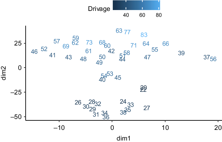
Figure 1. Driver age embedding reduced to two dimensions using the t-SNE technique.

The figure shows that the embeddings for the youngest age groups in the model (i.e. 20 and 22) cluster together, with two additional clusters relaying to the young adult and older adult ages apparent. Figure 2 shows the relationship of the embeddings (again in two dimensions derived using the t-SNE technique) to the driver age variable. The interpretation here is that the first dimension represents a schedule of claims rates according to age, with the rates starting off high at the youngest ages (i.e. above zero), dropping down in the middle ages mostly below zero) and then rising at the older ages (mostly above zero). The second dimension shows how the relationship between the claims rates at the younger and older ages might change by “twisting” the schedule of rates (i.e. if the rates at younger ages go down, those at older ages go up and vice versa). The embedding therefore seems to tie in with the intuition that the youngest and least experienced drivers will have similar high claims frequency experience, that more experienced but nonetheless young drivers will have the lowest claims rates and that the oldest drivers will again experience a rise in frequency.

Figure 2. Driver age embedding reduced to two dimensions using the t-SNE technique, plotted against the driver age variable.

That the learned embedding has an easy and useful interpretation was then shown by including the embedding in a simple GLM model in place of the categorical driver age variable, and this result is referred to in the table as GLM_embed. This application of transfer learning (i.e. reuse of a calibrated neural network component in another model) reduced the out-of-sample loss of the GLM relatively significantly, showing that the learned embedding has a meaning outside of the neural network, and, presumably, even better performance could be achieved by replacing all of the variables in the GLM with the corresponding embeddings. Since actuaries are more used to pricing personal lines business using GLMs, pre-training embeddings in a neural network which are then used within GLMs as additional parameter vectors seems like a promising strategy to be explored further.

A last illustration ^{Footnote 4} of the flexibility of neural networks builds upon the observation of Noll et al. (Reference Noll, Salzmann and Wüthrich2018) that including exposure as a feature component instead of a multiplicative constant results in a much more predictive model. The network denoted as NN_learned_embed implements this idea in two ways. Firstly, the exposure is input into the model via an embedding layer, in the same way as described above for the rest of the numerical features, by splitting the exposure variable into 46 groups, and estimating an 11-dimensional embedding for each of the 46 groups. Secondly, a secondary network is built (within the main network) to apply a multiplicative scaling factor to the policy exposure to produce a “learned exposure” which is used in place of the policy exposure to predict claims frequency. This network is shown in Figure 3.

Figure 3. Learned exposure network. A sub-network learns an exposure modifier factor, which is multiplied with the policy exposure to produce the learned exposure. The learned exposure is used in place of the policy exposure to predict claims frequencies.

Of the networks discussed, the learned exposure network by far outperforms the rest (note that including the exposure embedding but not the secondary network did not produce as optimal a result). To build some intuition, the average learned exposures are shown in Figure 4 plotted against the average exposures in the data, segmented by the number of claims. The figure shows that at the lowest level of exposures, the network has dramatically increased the level of exposure for those policies claiming at least once ^{Footnote 5} , as well as for multi-claimants, indicating that the time a policy spends in force is not an optimal exposure measure, and, indeed, a recent analysis of telematics data appears to indicate that distance travelled is a more optimal exposure measure (Boucher et al., Reference Boucher, Côté and Guillen2017).

Figure 4. Learned exposures, segmented by number of claims made, plotted against exposure.

2.2.1 Granular reserving using neural networks

IBNR reserves are generally calculated at the level of a line of business (LoB), which represents a homogenous portfolio with similar exposure to risk and types of claims. This high-level calculation is generally sufficient for solvency reporting and basic management information. However, a vexing problem in practice is the production of reserves for groupings of business lower than the LoB aggregation, since, on the one hand, these more granular calculations might reveal important information about the business such as particularly poorly performing segments, but on the other hand, the more granular data is often too sparse for the traditional chain-ladder calculations. One potential solution is the various credibility weighted extensions of the chain-ladder, see, for example, Bühlmann et al. (Reference Bühlmann, De Felice, Gisler, Moriconi and Wüthrich2009); Gisler and Wüthrich (Reference Gisler and Wüthrich2008); however, these have been developed only to the extent of a single level of disaggregation from the usual calculations.

A more recent approach is Wüthrich (Reference Wüthrich2018a) who extends the formulation of the chain-ladder as a regression model to incorporate features such as LoB, type of injury and age of the injured. The basic chain-ladder method uses the aggregated incurred or paid claims (or claim amounts) from accident period $i$ developed up to a point in time $j$ , ${C_{i,j}}$ , as the sole input feature into a regression model:

\begin{equation*}{\hat{C}}_{i,j+1}=f_j.C_{i,j}\end{equation*}

where ${\hat{C}}_{i,j+1}$ is the estimated claim amount for the next development period and ${f_j}$ is the so-called loss development factor (LDF) (after estimating ${\hat{C}}_{i,j+1}$ , the calculations are continued using the predicted value as the next feature for that accident year). This could be expressed in a functional form ${\hat{C}}_{i,j+1}=f(X).C_{i,j}$ , where $X$ is a feature vector containing only one feature, in this case, the development period $j$ . The insight of Wüthrich (Reference Wüthrich2018a) is to extend the feature space $X$ to include other components, namely, LoB, labour sector, accident quarter, age of the injured and body part injured, and then, to fit a neural network model to estimate the expanded function $f\!\left( X \right)$ . Once this function is estimated, it is used to derive LDFs at the level of granularity of the expanded feature vector $X$ , and the chain-ladder method can be applied as normal.

One complication is that as the data are disaggregated, the multiplicative structure of the model may fail if ${C_{i,j}}$ is zero (i.e. no claims have been incurred/paid in accident period $i$ up to a point in time, $j$ ). Two approaches are possible. A simpler approach is to calculate a second chain-ladder model, fit for each LoB separately, which projects the total aggregated ${C_{i,j}}$ to ultimate using modified LDFs that allow only for the development of claims from zero and a more complicated approach would allow for an intercept in the regression model that is only calculated if ${C_{i,j}}$ is zero, that is, $\smash{{\hat{C}}_{i,j+1}=f_j.C_{i,j}+1_{C_{i,j}=0}.g_j}$ , where ${1_{{C_{i,j}} = 0}}$ is an indicator function that takes the value of one when ${C_{i,j}} = 0$ and ${g_j}$ is an intercept term relating to development time $j$ .

The neural network used in Wüthrich (Reference Wüthrich2018a) had a single layer of 20 neurons and used the hyperbolic tangent activation function. Comparing the neural network and chain-ladder reserves to the true underlying dataset, it was found that the neural network reserves were almost perfectly accurate for three of the four LoBs considered, and more accurate than the chain-ladder reserves, while, on the fourth line, both the neural network and chain-ladder reserves were over-stated, the former more than the latter. The results of the neural network approach were also quite accurate at the level of age, injury code, and claims code, which, besides for allowing for a more detailed understanding of the aggregate IBNR requirements, also allows for the production of detailed management information, as well as input into pricing. To explain the outperformance of the neural network model, Wüthrich (Reference Wüthrich2018a) notes that the neural network is inherently a multivariate approach that leverages similar patterns in the data across LoBs, whereas the chain-ladder is applied to each LoB separately.

In summary, the neural network chain-ladder model is a combination of a traditional actuarial method with a machine learning method, and this paradigm of combining traditional techniques with neural networks will be noted throughout this section.

We refer the reader to the appendices in Wüthrich (Reference Wüthrich2018a) for code to fit the model in Keras.

2.2.2 Individual claims simulation machine

Gabrielli and Wüthrich (Reference Gabrielli and Wüthrich2018) make an important contribution by providing software to simulate individual claims for the purpose of testing individual claims reserving methods. Although the methodology used to simulate is not directly applicable to reserving in practice (since it focuses on modelling a claims dataset that has already fully developed), this research is mentioned here because it uses several neural networks to simulate the complicated individual claims data, and, more importantly, because the availability of test datasets appears to be an important step in advancing the state of the art in machine learning. Wüthrich (Reference Wüthrich2018a) contains code to simulate the claims data for the neural network chain-ladder model using the individual claims simulation machine.

2.2.3 DeepTriangle

A different approach to IBNR reserving appears in Kuo (Reference Kuo2018b), with an associated R package (Kuo, Reference Kuo2018a), who applies many of the concepts mentioned in Section 4 of Part 1 of this paper to a large triangle dataset provided by Meyers and Shi (Reference Meyers and Shi2011). This dataset, which is based on Schedule P submissions of many P&C companies in the USA and is available on the Casualty Actuary Society website, contains paid and incurred claims triangles covering the accident years 1988–1997, the development observed on those triangles in the subsequent years 1998–2006, and earned premiums relating to the accident years. For input to the DeepTriangle model, the incremental paid claims and total outstanding loss reserve triangles were normalised by earned premium, so, effectively, the model is fit to incremental paid and total outstanding loss ratios.

The proposed network combines embedding layers, for the company code categorical feature, and recurrent neural networks (RNNs, namely a gated recurrent unit or GRU, described in Chung et al. (Reference Chung, Gulcehre, Cho and Bengio2015), which is similar to an LSTM unit) for the variable length accident year development up to development period $j$ with fully connected layers and is amongst the most complicated of the architectures surveyed in this section ^{Footnote 6} . The network is a so-called multi-task variant on the single output networks seen until now, with the main goal of the network to predict unseen incremental paid claims, but with a secondary goal of predicting the outstanding reserve balances at each point. Multi-task networks often generalise better than single-task networks, since the shared parameters learned by the model are constrained towards good (i.e. predictive) values (Goodfellow et al., Reference Goodfellow, Bengio and Courville2016). The DeepTriangle model was fit to data from 50 companies in four lines of business, namely, Commercial and Private Auto, Workers Compensation and Other Liability. To fit the network, an initial training run was performed using the data of calendar year 1995 as a training set and 1996–1997 as a validation (out-of-sample) set. The number of epochs to produce the minimal validation set error was recorded, and the model was refit to the data of calendar year 1997 in a second training run. Each extra diagonal predicted by the model was added back to the triangle as input into the next prediction of the model, and the process was followed until the lower triangles were derived. These results show that DeepTriangle network outperforms the traditional Mack and GLM formulations of the chain-ladder on all lines, and is outperformed only on a single line, Commercial Auto, by one of the Bayesian models in Meyers (Reference Meyers2015).

The comparison of DeepTriangle to the traditional chain-ladder models is somewhat unfair, for two reasons. Firstly, actuaries in practise would not generally apply the chain-ladder model without carefully considering the potential for the LDFs to change over the accident years, and secondly, DeepTriangle is a multivariate model fit on 50 triangles of two variables each (paid and outstanding claims), whereas the chain-ladder is fit on a single triangle at a time. A more meaningful comparison would be to a multivariate extension of the chain-ladder, whether a traditional model such as Gisler and Wüthrich (Reference Gisler and Wüthrich2008) or a neural model such as Wüthrich (Reference Wüthrich2018a). Another practical issue to consider is that the model performance probably depends on the volume of data used (i.e. 50 triangles of claims paid and outstanding) and, in practice, only large multi-line insurers would have sufficient data to calibrate this type of network. However, having noted these concerns, the DeepTriangle network, and similar variants which are possible using different combinations of the neural network building blocks discussed in Section 3, represents an opportunity for greater accuracy in and automation of the loss reserving process.

Whereas DeepTriangle works on the level of aggregate claims triangles, a somewhat similar approach applied to individual claims is Zarkadoulas (Reference Zarkadoulas2017), who studies the use of neural networks to predict individual claims payments, using the time series of reserves and payments made to date on each individual claim as a feature vector fed into a shallow neural network. Separate networks are calibrated to estimate the $j - 1$ development periods through which an individual claim develops in a triangle. Since the feature vector relies on the time series of claims development to date, it would seem that the method can only be applied to claims already reported (i.e. to estimate Incurred But Not enough Reported) and the details of how this is extended to IBNR claims are unfortunately not clear. In any event, the results of the exercise are very similar to those of the chain-ladder that is also applied.

Code to apply the DeepTriangle model is available in Kuo (Reference Kuo2018a).

2.2.4 Uncertainty

In closing this section, we note that a key issue in the estimation of IBNR reserves is providing an estimate of the uncertainty of the reserve estimates, and we refer the reader to the seminal work of Mack (Reference Mack1993) and England and Verrall (Reference England and Verrall1999) for two foundational approaches to this problem. Within the neural network literature, which has focussed on “best estimate” approaches, relatively less attention has been given to the problem of uncertainty quantification and there does not appear to be a consensus on the most optimal method among the proposed approaches (for the interested reader, two noteworthy techniques appear in Gal and Ghahramani (Reference Gal and Ghahramani2016) and Lakshminarayanan et al. (Reference Lakshminarayanan, Pritzel and Blundell2017)). Perhaps for this reason, the papers covered in this survey do not discuss solutions to the problem of uncertainty estimation, which remains a key research issue that should be addressed by actuaries wishing to apply deep learning techniques practically.

2.3.1 v-a Heatmaps

Wüthrich (Reference Wüthrich2017) introduced the concept of so-called velocity–acceleration (“v-a”) heatmaps. An empirical global positioning system (GPS) location dataset, recorded at a 1-second frequency, of 1 753 drivers and 200 recorded trips was used to estimate the velocity and acceleration (i.e. change in average speed) of the driver at each time point. The various speed profiles were distributed into groups depending on the speed, for example, low speeds between 5–20 km/h and highway speeds between 80 and 130 km/h. Two-dimensional heatmaps, with the x-axis representing velocity in km/h and the y-axis representing acceleration in m/s² of the density of the empirical observations, were constructed (note that a discrete approach to building the heatmap was taken and another possible approach is two-dimensional kernel density estimation). An example heatmap generated using the code provided by Wüthrich (Reference Wüthrich2018b) is shown in Figure 5.

Figure 5. v-a heatmap generated using the code provided by Wüthrich (2018c). The x-axis is speed, the y-axis is acceleration and the coloured scale shows the empirical density at each point.

An important practical result is in Gao et al. (Reference Gao, Meng and Wüthrich2018), who provide a statistical analysis showing that around 300 minutes of telematics data is generally enough volume to build a stable v-a heatmap in the 5–20 km/h category.

Wüthrich (Reference Wüthrich2017) and Gao and Wüthrich (Reference Gao and Wüthrich2017) then apply several unsupervised learning methods to the v-a heatmaps. In Section 3 of Part 1 of this paper, unsupervised learning was defined as the task of finding meaningful patterns within feature vectors X, which can then be used to further understand the data. In this case, the v-a heatmap is the feature vector comprising the empirical density of observations for each velocity and acceleration group. Wüthrich (Reference Wüthrich2017) applied the k-means algorithm (see James et al. (Reference James, Witten, Hastie and Tibshirani2013) for details) to derive 10 discrete clusters into which the 1 753 v-a heatmaps were classified. Gao and Wüthrich (Reference Gao and Wüthrich2017) took a different approach and looked to derive low-dimensional continuous summaries of the v-a heatmaps using principal components analysis (PCA) and shallow and deep auto-encoder neural networks. PCA was applied to a matrix comprising a row for each driver and a column for each combination of velocity and acceleration, and it was found that relatively good summaries of the heatmaps could be formed using only two of the principal components. The shallow ^{Footnote 7} auto-encoder (called a bottleneck network in this study) consisted of a hidden layer of two neurons, with hyperbolic tangent activation functions and ending in a soft-max layer. The deep auto-encoder consisted of an extra layer of seven neurons before and after the two neuron layer. The auto-encoder was trained using greedy unsupervised learning (Goodfellow et al., Reference Goodfellow, Bengio and Courville2016, p. Chapter 15) (see Section 4 of Part 1 for more details). Both neural networks were trained using the Kullback–Leibler (K–L) loss function, which, in summary, measures how far apart two distributions are, and amounts to maximising the likelihood of a multinomial distribution on the data. On all the metrics considered, the deep auto-encoder network outperformed the shallow auto-encoder, which in turn outperformed the PCA.

Finally, Gao et al. (Reference Gao, Meng and Wüthrich2018) use the features extracted from the v-a heatmaps in a GAM of claim counts. The dataset considered in this study consists of 1 478 divers with 3 332 years of exposure and a relatively high claims frequency of 23.56%. All four methods described above for extracting features from the v-a heatmaps were applied to this new dataset. When applying the k-means algorithm, the number of clusters (i.e. means) were chosen using 10-fold cross-validation (see Friedman et al. (Reference Friedman, Hastie and Tibshirani2009, p. Chapter 7) for more details) to estimate the out-of-sample Poisson deviance. The continuous (PCA and auto-encoder) features were included directly in the GAM. In a stunning result (recall that the features were extracted in an unsupervised manner), the continuous features are not only highly predictive but, by themselves, produce a better out-of-sample deviance than the models including the traditional features of driver’s age and car’s age.

While Gao et al. (Reference Gao, Meng and Wüthrich2018) do not attempt to explain why the features estimated using unsupervised methods are highly predictive in a supervised context, some understanding is possible based on Goodfellow et al. (Reference Goodfellow, Bengio and Courville2016, p. Chapter 15), who are concerned, in Section 15.1, primarily with greedy unsupervised pre-training, and explain that “the basic idea is that some features that are useful for the unsupervised task may also be useful for the supervised learning task,” that is, the unsupervised representation that is learned may capture information about the problem that the supervised learning algorithm can access.

2.3.2 Analysis using Keras

We show in this section how the v-a heatmaps can be analysed using auto-encoders in Keras. For input data, 10,000 heatmaps were generated using the simulation machine of Wüthrich (Reference Wüthrich2018b). Since in any event the data are summarised in the parameters of the simulation machine, we do seek to add much insight in understanding these data, but rather to understand how auto-encoders can be applied.

Two different types of auto-encoder were applied – a basic fully connected auto-encoder, as well as a convolutional auto-encoder. The convolutional auto-encoder uses several layers of learned convolutional filters to derive the encoded heatmap, instead of fully connected layers, and rebuilds the output from the encoded heatmap using transposed convolutions, which are effectively the reverse operation. Both types of auto-encoders were applied with hyperbolic tangent activations. We show the choice of structure for these auto-encoders in Tables 2 and 3.

Table 2. Structure of fully connected auto-encoder applied to v-a heatmaps

Table 3. Structure of convolutional auto-encoder applied to v-a heatmaps. For definition of the terms used in this table, see Section 4.3.1 of Part 1

To train these, a process of greedy unsupervised learning was followed. First, the outer layers of each auto-encoder were trained. Then, the weights derived in the first step were held constant (i.e. frozen) and a new layer was added and trained. This process was followed until the dimensionality of the heatmap had been reduced to a 1 × 2 vector of codes. The fully connected auto-encoder used two hidden layers between the input and the encoding, whereas the convolutional auto-encoder used three layers of filters. The encoded heatmaps are shown in Figures 6 and 7, where the two-dimensional encoded values have been grouped according to the quantiles of the encoding distribution. Whereas the codes produced using the fully connected auto-encoder are relatively highly correlated, with a correlation coefficient of 0.85, the codes produced by the convolutional auto-encoder have a much lower correlation of 0.29, implying that the factors of variation describing the heatmap have been better disentangled by the convolutional auto-encoder. The mean heatmaps in each quantile group are shown in Figures 8 and 9. The interpretation of the learned codes is easier in the latter figure – moving from right to left in the encoded distribution shifts density to a higher velocity, and from bottom to top shifts probability density from a wide area to several key points – whereas in the former figure, it is harder to assign a definite interpretation. We conclude from this exercise that convolutional auto-encoders are a promising technique that should be explored further in the context of telematics data. In particular, it would be interesting to investigate the results of including the codes from the convolutional model in a claims frequency model, as done with the codes from a fully connected auto-encoder in the study of Gao et al. (Reference Gao, Meng and Wüthrich2018).

Figure 6. Heatmaps encoded using a fully connected auto-encoder and grouped by quantile of the encoded distribution.

Figure 7. Heatmaps encoded using a convolutional auto-encoder and grouped by quantile of the encoded distribution.

Figure 8. Mean heatmap for each group shown in Figure 6.

Figure 9. Mean heatmap for each group shown in Figure 7.

2.3.3 Other sources

To summarise the approach discussed to this point, the high-dimensional and high-frequency telematics data are first summarised in a v-a heatmap, which, compared to classical features in motor pricing, is itself a relatively high-dimensional feature. The v-a heatmap can be used as a feature in GLM rating models once the data have been summarised using dimensionality reduction techniques. During the (double) summarisation of the data, potentially some information is lost, and, therefore, with enough data, one might expect the application of RNNs to the GPS data, either raw or less summarised than the v-a heatmaps, to outperform approaches that rely on summarised data. Therefore, for completeness, in this section, we discuss several recent applications of neural networks to GPS or telematics data from outside the actuarial literature.

De Brébisson et al. (Reference De Brébisson, Simon, Auvolat, Vincent and Bengio2015) discuss several deep networks applied to the problem of predicting taxi destinations based on variable length GPS data, as well as meta-data describing driver, client and trip features, covering 1.7 million trip records of taxis in Portugal. These meta-data were modelled using embedding layers, while several approaches were taken to model the GPS data directly. The simplest approach (which won the competition) was to use a fixed amount of the GPS data as an input directly to a feed-forward network. More complicated models recognised that the variable length GPS data could be modelled using RNNs, and, therefore, RNN and LSTM networks were calibrated on the raw GPS data, with the output of these networks fed into the same network structure just mentioned (i.e. including embedding layers for the meta-data). A variant of these was the highest ranked model within the authors’ test set.

Dong et al. (Reference Dong, Li, Yao, Li, Yuan and Wang2016) find that deep learning applied directly to GPS data for the task of characterising driving styles does not perform well (whereas in De Brébisson et al. (Reference De Brébisson, Simon, Auvolat, Vincent and Bengio2015), the goal is to predict the destination, that is, the output is in the same domain as the input data). Thus, in a manner similar to Wüthrich (Reference Wüthrich2017), they rely on a data summary approach (which Dong et al. (Reference Dong, Li, Yao, Li, Yuan and Wang2016) refer to as a “double windowing” approach) to process the raw GPS data, which is applied in two steps. First, the raw GPS data are segmented into trip “windows,” meaning to say, that segments of length 256 seconds are selected out of the raw GPS data and, within those segments of 256 seconds of GPS data, the following basic features are calculated: speed and acceleration, and the change in each of these components over time, and angular momentum. Then, the segments of 256 seconds are further segmented into a second measurement “window” of 4 seconds, and within each measurement window, and for each of these basic features, summary statistics (the mean, standard deviation, minimum, maximum, median, and 25th and 75 th percentiles) are calculated. This approach thus leads to a matrix (or feature map) of basic movement statistics for each trip window, where each row represents a movement statistic, and each column represents time (i.e. a new observation window). Since driver behaviour manifests itself over time, one would expect that the movement statistics would have some sort of temporal structure, which is analysed using either convolutional neural networks (CNNs) or RNNs, with a detailed description of the application of both methods in the paper. Notably, cross-correlation between features is not allowed for in either of these models, and, given the performance of the v-a heatmaps discussed above, it would seem that this is an omission. The networks are trained on a dataset consisting of driver trips with the goal of classifying the driver correctly; in a first example, only 50 drivers from the dataset are used, and 1000 drivers are used in the second experiment. A variant of the RNN network outperformed all other approaches, including a machine learning baseline. Investigating the learned features, the study concludes that the network has automatically identified driving behaviour, such as slowing down for sharp turns, or high-speed driving on straight roads.

Dong et al. (Reference Dong, Yuan, Yang, Li and Zhang2017) extend the model of Dong et al. (Reference Dong, Li, Yao, Li, Yuan and Wang2016) in several ways, in a new network they call Autoencoder Regularized deep neural Network (ARNet). Their network design, applied to the same movement statistic feature matrix, relies exclusively on RNNs (specifically, the GRU of Chung et al. (Reference Chung, Gulcehre, Cho and Bengio2015)) for driver classification, in a similar setup to Dong et al. (Reference Dong, Li, Yao, Li, Yuan and Wang2016), but also includes an auto-encoder branch within the network that aims to reconstruct the (hidden) layer of the network that represents driving style. The idea of adding the auto-encoder to the classification model is explained as follows: the auto-encoder is regularised (i.e. the auto-encoder representation is shrunk towards zero), which should improve the generalisation of the classification branch of the network to unseen data, and the classification branch includes prior information about the driver within the network structure, which should improve the auto-encoder representation of driving style. ARNet outperforms on the two tasks tested in the research – driver classification and driver number estimation, compared to both the shallow and deep machine learning baselines also tested in that research.

Wijnands et al. (Reference Wijnands, Thompson, Aschwanden and Stevenson2018) use an LSTM network to predict whether a driver’s behaviour has changed, based on sequences of telematics data, containing, for each sequence, counts of acceleration, deceleration and speeding events. An LSTM is trained for each driver to classify these sequences of events as belonging to one of three benchmarks, one for safe driving, one for unsafe driving and one for the driver under consideration, where the benchmarks are themselves based on an insurer’s proprietary scoring algorithm. If driver behaviour changes, then the LSTM classification is shown to be able to classify the driver’s behaviour as arising from the benchmarks, and not as similar to the driver’s own previous driving style.

We refer the interested reader to the review in Ezzini et al. (Reference Ezzini, Berrada and Ghogho2018) for more references of applying machine learning and statistical techniques to these types of data.

2.4.1 Analysis using Keras

In this section, we attempt to produce similar results with Keras, noting that the relatively complicated genetic evolution optimisation scheme of Hainaut (Reference Hainaut2018a) is not supported within the Keras package, but only backpropagation and associated optimisers are supported. We also note that the network in the previous example benefits from substantial manual feature engineering, in that the network is fit only to the time-varying component of mortality, and, furthermore, the first hidden layer is only locally connected. The paradigm of representation learning would, however, seem to indicate that the network should be left to figure out these features by itself, and perhaps arrive at a more optimal solution in the process.

Therefore, a first attempt at the problem of mortality forecasting applied greedy unsupervised learning to train fully connected auto-encoders on mortality data (the central rate of mortality, ${m_x}$ ) from England and Wales in the period 1950–2016, covering the ages 0–99, sourced from the Human Mortality Database (HMD) (Wilmoth & Shkolnikov, Reference Wilmoth and Shkolnikov2010). The training dataset was taken as mortality in the period 1950–1999, and the test dataset was in the period 2000–2016, and the logarithm of ${m_x}$ was scaled so as to lie in the interval [0, 1]. The neural networks were fit exclusively on this scaled dataset and were compared to a baseline Lee–Carter model fit directly to the raw ${m_{x,t}}$ using the gnm package (Turner & Firth, Reference Turner and Firth2007), and forecast using exponential smoothing as implemented in the forecast package Hyndman et al. (Reference Hyndman, Athanasopoulos, Razbash, Schmidt, Zhou, Khan and Wang2015).

The auto-encoders used hyperbolic tangent activations, and each layer was fit for 50,000 epochs using the Adam optimiser (Kingma & Ba, Reference Kingma and Ba2014) implemented in Keras, with a learning rate schedule hand designed to minimise the training error. Table 4 shows the structure of the auto-encoder. The encoded mortality curves were forecast using a random walk with drift to produce forecasts for each of the years in the period 2000–2016. These results, referred to as Auto-encoder, as well as the Lee–Carter baseline are shown in Table 5. The auto-encoder forecasts outperform the baseline Lee–Carter model, showing that a viable auto-encoder model can be fit in Keras without too much manual feature engineering.

Table 4. Structure of fully connected auto-encoder applied to mortality data

Table 5. Mortality forecasting – out-of-sample mean squared error (MSE)

However, it is important to note that fitting the auto-encoders is difficult and computationally expensive, and the results produced on the out-of-sample data can be variable, with worse performance than reported in the table possible. One way of reducing the variability is to average the results of several deep models (Guo & Berkhahn, Reference Guo and Berkhahn2016), but a comparison of the resulting ensemble model to the Lee–Carter model would be unfair. Therefore, we also demonstrate a different approach using deep learning for mortality forecasting and, in the following, show how the Lee–Carter model could be fit and extended using embedding layers.

The Lee–Carter model can be expressed in functional form as

\begin{equation*}\ln ({\mu _{x,t}}) = f\left( {x,t} \right) = {a_x} + {\kappa _t}.{b_x}\end{equation*}

\hspace*{10pt}\begin{equation*}{a_x} = g\left( x \right)\left\{\!\! {\begin{array}{*{20}{c}}{{a_1},\ x = 1}\\{{a_2},\ x = 2}\\{...}\\{{a_n},\ x = n}\end{array}} \right.\hspace*{-15pt}\end{equation*}

up to a maximum age $n$ , and similarly for ${\kappa _t}$ and ${b_x}$ . Rather than specify this particular functional form, a neural network can be used to learn the function $f\left( {x,t} \right)$ directly, by using age and calendar year as predictors in a neural network that is then trained to predict mortality rates. This network was fit on the same dataset as the auto-encoders and consisted of an embedding layer for age and two hidden layers of 32 neurons with the ReLu activation (between each hidden layer, dropout (Srivastava et al., Reference Srivastava, Hinton, Krizhevsky, Sutskever and Salakhutdinov2014) was applied to regularise the network). The year variable was left as a numerical input to the network and is used to forecast future mortality rates. The structure of this network is shown in Table 6 and is referred to as Deep_reg in Table 5.

Table 6. Structure of neural network fit to the mortality data for England and Wales

A similar network was fit to the entire HMD dataset at once, with an embedding for the country to which the mortality rates relate. The structure of this network is shown in Table 7 and is referred to as Deep_reg_hmd in Table 5. It can be seen that of all the networks tested, Deep_reg outperforms the others, followed closely by Deep_reg_hmd. However, as discussed next, on the long-term forecast of rates in 2016 (forecast using data up to 1999), the Deep_reg_hmd network outperforms the other networks, followed closely by the auto-encoder.

Table 7. Structure of neural network fit to the mortality data for the HMD dataset

Figures 10 and 11 show the forecasts of mortality in 2000 (i.e. a one-year horizon) and 2016 (i.e. a 16-year horizon) produced using the models described in this section. All of the models are quite close to actual mortality in 2000, but some of the forecasts diverge compared to actual mortality in 2016. In 2016, the Deep_reg_hmd forecasts follow the actual mortality curve closely at almost all ages, while the Lee–Carter and auto-encoder forecasts appear too high in middle age. On closer inspection, the Deep_reg forecasts in 2000 are quite variable at some ages, and by 2016 have degraded over time and do not appear demographically reasonable, whereas the Deep_reg_hmd forecasts have remained demographically reasonable.

Figure 10. Forecasts of mortality in 2000 using the models described in this section, log scale.

Figure 11. Forecasts of mortality in 2016 using the models described in this section, log scale.

The learned embedding for age from the Deep_reg_hmd network is shown in Figure 12. The dimensionality of the embedding was reduced to 2 dimensions from 20 dimensions using PCA. The first dimension is immediately recognisable as the basic shape of a modern lifetable, which is effectively the function ${a_x}$ fit by the Lee–Carter model. The second dimension appears to describe the relationship between early childhood, young middle age, late middle age and old-age mortality, with early childhood and late middle age mortality steepening as young middle age and old-age mortality declines, and vice versa.

Figure 12. Age embedding from the Deep_reg_hmd model, with dimensionality reduced using PCA.

We conclude from this brief study of mortality that deep neural networks appear to be a promising approach for modelling and forecasting population mortality. The neural network model presented in this sub-section is discussed in detail in Richman and Wüthrich (Reference Richman and Wüthrich2018) ^{Footnote 9} .