


1. Introduction
Exploration and colonisation of the Martian environment have recently gained attention from many countries with multiple road maps for potential manned flights to Mars proposed (see e.g. Daniluk et al. Reference Daniluk, Klyushnikov, Kuznetsov and Osadchenko2015; Igritsky & Mayorova Reference Igritsky and Mayorova2021; Palmer Reference Palmer2021). To achieve this goal, a sustainable and efficient means of exploration is required to understand the landscape, terrain, climate and resources on Mars. Aerial vehicles are preferred since they are not inhibited by the ground terrain, and can provide broad perspective and sampling of the environment with a reasonable balance between manoeuvrability, data resolution, price and manufacture challenges (Liu, Aono & Tanaka Reference Liu, Aono and Tanaka2013).
Flight is challenging on Mars, primarily due to the low density, which is approximately 1 % of Earth's density (Seiff & Kirk Reference Seiff and Kirk1977; Barlow Reference Barlow2008; Munday et al. Reference Munday, Taira, Suwa, Numata and Asai2015), and consequently low operational Reynolds numbers (e.g.  $O(10^2\unicode{x2013}10^4$) for small-scale vehicles (Shrestha et al. Reference Shrestha, Benedict, Hrishikeshavan and Chopra2016; Bluman et al. Reference Bluman, Pohly, Sridhar, Kang, Landrum, Fahimi and Aono2018). As such, traditional rotor-wing and fixed-wing aircraft are impractical or require substantial resources to stay airborne for a long duration due to the low lift coefficient (Sullivan et al. Reference Sullivan, Greeley, Kraft, Wilson, Golombek, Herkenhoff, Murphy and Smith2000; Shrestha et al. Reference Shrestha, Benedict, Hrishikeshavan and Chopra2016; Eldredge & Jones Reference Eldredge and Jones2019; Pohly et al. Reference Pohly, Kang, Landrum, Bluman and Aono2021). For example, the Mars helicopter ‘Ingenuity’ uses rotor blades to achieve flight, but has a low flight duration of less than 3 minutes (Tzanetos et al. Reference Tzanetos2022). Bio-inspired flapping wings, on the other hand, have been identified as a potential solution, as insects and birds operate in the low Reynolds number regime on Earth, generating efficient lift relative to their sizes with which fixed-wing or rotatory-wing vehicles cannot compete (Pesavento & Wang Reference Pesavento and Wang2009; Shyy et al. Reference Shyy, Aono, Chimakurthi, Trizila, Kang, Cesnik and Liu2010; Eldredge & Jones Reference Eldredge and Jones2019), and potentially resulting in a longer flight duration.
One of the important features of bio-inspired flapping wings is their ability to generate high lift at low Reynolds numbers (Pesavento & Wang Reference Pesavento and Wang2009; Shyy et al. Reference Shyy, Aono, Chimakurthi, Trizila, Kang, Cesnik and Liu2010; Eldredge & Jones Reference Eldredge and Jones2019; Liu, Wang & Liu Reference Liu, Wang and Liu2024). The high lift is achieved by a few unsteady mechanisms, such as vortices around the wing (Dickinson, Lehmann & Sane Reference Dickinson, Lehmann and Sane1999; Shyy et al. Reference Shyy, Aono, Chimakurthi, Trizila, Kang, Cesnik and Liu2010), added mass (Sane & Dickinson Reference Sane and Dickinson2001; Chin & Lentink Reference Chin and Lentink2016), rapid pitching rotational circulation (Dickinson et al. Reference Dickinson, Lehmann and Sane1999; Shyy et al. Reference Shyy, Aono, Chimakurthi, Trizila, Kang, Cesnik and Liu2010; Chin & Lentink Reference Chin and Lentink2016), clap and fling (Weis-Fogh Reference Weis-Fogh1973; Shyy et al. Reference Shyy, Aono, Chimakurthi, Trizila, Kang, Cesnik and Liu2010; Chin & Lentink Reference Chin and Lentink2016), passive/active control through geometries and appendages (Carruthers et al. Reference Carruthers, Thomas, Walker and Taylor2010; Tian et al. Reference Tian, Tobing, Young, Lai, Walker, Taylor and Thomas2019; Duan & Wissa Reference Duan and Wissa2021; Othman et al. Reference Othman, Zekry, Saro-Cortes, Lee and Wissa2023), and a variety of synchronisations (Bomphrey et al. Reference Bomphrey, Nakata, Phillips and Walker2017; Huang et al. Reference Huang, Bhat, Yeo, Young, Lai, Tian and Ravi2023) and passive deformations (Nakata & Liu Reference Nakata and Liu2012; Kang & Shyy Reference Kang and Shyy2013; Tian et al. Reference Tian, Luo, Song and Lu2013; Shahzad et al. Reference Shahzad, Tian, Young and Lai2018a,Reference Shahzad, Tian, Young and Laib). The vortices include the leading-edge vortex (LEV), the trailing edge vortex, the tip/root vortex and the incoming/wake vortex. Among these vortices, the LEV is the most prominent flow structure. The LEV undergoes delayed stall or even absence of stall so that it remains attached to the leading edge during the middle stroke (Ellington et al. Reference Ellington, van den Berg, Willmott and Thomas1996; Liu et al. Reference Liu, Ellington, Kawachi, Van Den Berg and Willmott1998; Chin & Lentink Reference Chin and Lentink2016, Reference Chin and Lentink2019; Hawkes & Lentink Reference Hawkes and Lentink2016). The delayed stall and absence of stall are responsible for most of the lift generation during the translational phase of the wing (Chin & Lentink Reference Chin and Lentink2016). The tip vortex also contributes to the aerodynamic force as it creates a low-pressure area near the wing tip. It can interact with the LEV and generate a wake structure by the downward and radial movement of the tip vortex and the root vortex (Shyy et al. Reference Shyy, Aono, Chimakurthi, Trizila, Kang, Cesnik and Liu2010). Advanced wing rotation (pitching), with the wing flipping before stroke reversal, enhances lift generation by generating circulation in the surrounding fluid and stabilising the LEV with centripetal and Coriolis accelerations (Lentink & Dickinson Reference Lentink and Dickinson2009; Chin & Lentink Reference Chin and Lentink2016). The wake capture mechanism accounts for a large potion of the aerodynamic force during pitch reversal (Lua et al. Reference Lua, Lee, Lim and Yeo2017; Wang et al. Reference Wang, Han, Zhu, Liu, Deng and Dong2018). The clap and fling mechanism produces lift through generating jet flows where the leading edges of the wings touch before the wings rotate around the leading edge, closing the gap between the wings and creating a downward jet; the wings then rotate around the trailing edge to achieve the fling open, generating a downward jet to fill the gap (Weis-Fogh Reference Weis-Fogh1973; Chin & Lentink Reference Chin and Lentink2016). There are vortices associated with the flap and fling mechanisms, as detailed in Chin & Lentink (Reference Chin and Lentink2016). The flexibility enhances the lift generation through increasing the effective pitching angle or adjusting the phase between pitching and stroke motions as results of the interplay between the inertia, aerodynamic and elastic forces (Dai, Luo & Doyle Reference Dai, Luo and Doyle2012; Tian et al. Reference Tian, Luo, Song and Lu2013; Huang et al. Reference Huang, Bhat, Yeo, Young, Lai, Tian and Ravi2023). The flow control strategies improve the flight performance by manipulating the vortex kinematics and dynamics around the wing through leading/trailing edge serrations, wing shape, appendages, slotted wing tips, surface structures, motions, etc. (e.g. Othman et al. Reference Othman, Zekry, Saro-Cortes, Lee and Wissa2023; Jin et al. Reference Jin, Wang, Ravi, Young, Lai and Tian2024). More details of the high lift generation and flow controls can be found in the aforementioned references. To summarise, the aerodynamic force generation of a flapping wing is highly dependent on a variety of factors, such as wing kinematics, geometries and structural parameters (see e.g. Ansari, Knowles & Zbikowski Reference Ansari, Knowles and Zbikowski2008; Nagai & Isogai Reference Nagai and Isogai2011; Taha, Hajj & Nayfeh Reference Taha, Hajj and Nayfeh2012; Shahzad et al. Reference Shahzad, Tian, Young and Lai2016).
The effects of compressibility have attracted the interest of researchers and engineers due to space exploration applications, especially UAV development for Martian flight due to the low density environment (see e.g. Liu et al. Reference Liu, Aono and Tanaka2013; Igritsky & Mayorova Reference Igritsky and Mayorova2021; Tzanetos et al. Reference Tzanetos2022). The lift force of a hovering wing,  $F_L$, can be written as
  $F_L=mg=0.5\rho _\infty U^2 A C_L$, where
  $m$ is the mass,
  $g$ is the gravitational constant,
  $\rho _\infty$ is the density of air,
  $A$ is the area of the wing,
  $U$ is the reference operating velocity, and
  $C_L$ is the lift coefficient. There are three important changes in the environment if the same wing (on Earth) is operated on Mars: the gravitational constant, the density of the atmosphere and the dynamic viscosity. Specifically, the gravitational constant, the air density and the dynamic viscosity on Mars are approximately
  $33\,\%$,
  $1\,\%$ and
  $73\,\%$ of those on Earth, respectively (Seiff & Kirk Reference Seiff and Kirk1977; Almeida et al. Reference Almeida, Parteli, Andrade and Herrmann2008; Barlow Reference Barlow2008; Munday et al. Reference Munday, Taira, Suwa, Numata and Asai2015). In order to support the same mass, on Mars the wing is required to operate at a velocity approximately six times greater than on Earth if
  $C_L$ is to remain the same. Another important consideration is the Reynolds number, which is defined as
  $Re = \rho _\infty U \bar {c}/\mu = 2 m g \bar {c}/(\mu A U C_L)$ or
  $\bar {c} \sqrt {2\rho _\infty mg}/(\mu \sqrt {A C_L})$, where
  $\bar {c}$ is the mean chord of the wing, and
  $\mu$ is the fluid viscosity. Therefore, scaling the force by increasing the velocity to compensate for the aerodynamic decrease due to the low-density environment ultimately decreases the Reynolds number. This is different from classical cases where increasing the velocity to increase the payload results in an increase in the Reynolds number. In addition, the flight endurance can be estimated by following Hawkes & Lentink (Reference Hawkes and Lentink2016) as
  $T_{en}=E_{in}\eta /(0.5\rho _\infty U^3 A C_{pow}) = E_{in}\eta C_L/(mg U C_{pow})$ or
  $E_{in}\eta C_L^{3/2}\sqrt {\rho _\infty A}/[\sqrt {2}(mg)^{3/2}C_{pow}]$, where
  $E_{in}$ is the total energy supply, including battery and other energies,
  $\eta$ is the compound efficiency of actuators, electronics and mechanical transmission mechanisms, and
  $C_{pow}$ is the aerodynamic power coefficient. From the perspective of aerodynamics, a lower-density environment means a lower endurance, which could be compensated by improving the lift coefficient and/or reducing the power coefficient. Therefore, the cumulative result of low density, high operating speed and low sound speed on Mars results in the wing operating at a lower Reynolds number where compressibility effects could be significant. Such operating conditions have been demonstrated by the Ingenuity helicopter, where the Mach number based on the blade-tip velocity reaches speeds up to
  $Ma = 0.7$ (Tzanetos et al. Reference Tzanetos2022).
Previous studies have indicated that bio-inspired flight is feasible for low-density environments, such as Mars, due to proven success in low Reynolds number regimes (Bluman et al. Reference Bluman, Pohly, Sridhar, Kang, Landrum, Fahimi and Aono2018; McCain et al. Reference McCain, Pohly, Sridhar, Kang, Landrum and Aono2020; Wang, Tian & Liu Reference Wang, Tian and Liu2022b). However, the effects of highly compressible flows on lift as well as the flow physics associated with compressibility have not been well understood. To gain a better understanding, it is necessary to analyse these effects using basic scaling laws, which have been used to analyse force production (see e.g. Dewey et al. Reference Dewey, Boschitsch, Moored, Stone and Smits2013; Quinn, Lauder & Smits Reference Quinn, Lauder and Smits2014; Lee, Choi & Kim Reference Lee, Choi and Kim2015; Floryan et al. Reference Floryan, Van Buren, Rowley and Smits2017; Ayancik et al. Reference Ayancik, Zhong, Quinn, Brandes, Bart-Smith and Moored2019) and sound (Wang & Tian Reference Wang and Tian2020) generated by flapping wings/foils. Recently, scaling laws have been extended to bio-inspired flyers on Mars, with the assumption of incompressible continuous flows while the low-density feature of Martian atmosphere is reflected in the dynamic pressure estimation (see e.g. Bluman et al. Reference Bluman, Pohly, Sridhar, Kang, Landrum, Fahimi and Aono2018; Xiao & Liu Reference Xiao and Liu2020; Pohly et al. Reference Pohly, Kang, Landrum, Bluman and Aono2021; Veismann et al. Reference Veismann, Dougherty, Rabinovitch, Quon and Gharib2021). Based on previous studies,  $C_{L}= \mathbb {F}(St, \alpha, r_1, \varPi _{1-N})$, where
  $St$ is the Strouhal number,
  $\alpha$ is the angle of attack (AoA),
  $r_1$ is the first moment of the wing area, and
  $\varPi _{1-N}$ reflects the effects of the characteristic elastic force, flexibility, passive deformation, LEV strength and leading/trailing edge velocity (Kang et al. Reference Kang, Aono, Cesnik and Shyy2011; Nakata & Liu Reference Nakata and Liu2012; Tian et al. Reference Tian, Luo, Song and Lu2013; Lee et al. Reference Lee, Choi and Kim2015; Floryan et al. Reference Floryan, Van Buren, Rowley and Smits2017; Shahzad et al. Reference Shahzad, Tian, Young and Lai2018a,Reference Shahzad, Tian, Young and Laib; Addo-Akoto, Han & Han Reference Addo-Akoto, Han and Han2022). Recently, it was found that the peak of the lift generated by a flexible hovering wing drops approximately 20 % when the Mach number increases from 0.2 to 0.6 (Wang et al. Reference Wang, Tian and Liu2022b), indicating that the compressibility has a significant effect on the force generation by a flapping wing. Therefore, it is necessary to consider the effect of compressibility on the scaling laws for the force generated by bio-inspired flapping wings in the low-density environments by rewriting the lift coefficient as
  $C_{L}= \hat {\mathbb {F}}(St, \alpha, r_1, Ma, \varPi _{1-N})$.
In previous studies using scaling laws, the viscous effect is normally ignored (see e.g. Kang et al. Reference Kang, Aono, Cesnik and Shyy2011; Bluman et al. Reference Bluman, Pohly, Sridhar, Kang, Landrum, Fahimi and Aono2018). However, Senturk & Smits (Reference Senturk and Smits2019) showed that the force coefficients of a pitching foil depend on the Reynolds number according to  $\sqrt {Re}$, indicating that the contribution of the friction force to the lift and the drag can be estimated by using the laminar boundary layer model. However, the application of this model needs to be further explored in three-dimensional flapping wings undergoing stroke and pitching motion.
Here, we aim to develop a scaling law for the lift of a bio-inspired wing hovering in low-density compressible flows to understand how the lift is influenced by the Reynolds and Mach numbers, as well as the associated flow physics. In order to achieve this aim, we perform numerical modelling of a three-dimensional rigid wing undergoing hovering kinematics (including stroke and pitching motion) using an immersed boundary method solver (Wang et al. Reference Wang, Currao, Han, Neely, Young and Tian2017, Reference Wang, Tian and Liu2022b; Wang, Young & Tian Reference Wang, Young and Tian2024). We investigate the force generations by varying the Reynolds number from 200 to 6000, and the average wing-tip Mach number from 0.2 to 1.4. The AoA of the wing during the middle stroke is also varied from  $30^{\circ }$ to
  $60^{\circ }$. Apart from the aerodynamic forces, we also investigate pressure distributions, vortex structures and shock waves. Most importantly, we propose a unique scaling law for the lift of the wing based on the flow physics of flapping-wing dynamics.
2. Physical problem and numerical method
2.1. Physical problem and governing equations
To develop a scaling law for the lift of a bio-inspired wing hovering in low-density compressible flows, two distinct wing planforms are considered, including a rectangular wing and a bumblebee wing (see figure 1), to discuss the geometric impacts on the scaling law analysis and to verify its effectiveness. As a generic geometry and the most simple approach, rectangular wings have been used extensively to study the fundamental aerodynamic principles associated with flapping wings (see e.g. Dai et al. Reference Dai, Luo and Doyle2012; Carr, Chen & Ringuette Reference Carr, Chen and Ringuette2013; Kruyt et al. Reference Kruyt, van Heijst, Altshuler and Lentink2015). The bumblebee wing geometry was defined by Dudley & Ellington (Reference Dudley and Ellington1990) and has been utilised extensively in previous studies (see e.g. Sun & Xiong Reference Sun and Xiong2005; Tobing, Young & Lai Reference Tobing, Young and Lai2013, Reference Tobing, Young and Lai2017). These wings have span length  $R$, and average chord
  $\bar {c}$. The aspect ratio (
 $\varLambda$) of the wing is
  $\varLambda = R/\bar {c}$. Here,
  $\varLambda =2$ is considered for the rectangular wing cases, while
  $\varLambda =3.3$ is utilised for the bumblebee wing to maintain similarity to previous studies (Tobing et al. Reference Tobing, Young and Lai2013, Reference Tobing, Young and Lai2017). It is noted that
  $\varLambda$ of typical insect wings clusters around value 3.0 (Lentink & Dickinson Reference Lentink and Dickinson2009). Here, a lower
  $\varLambda$ is used for the rectangular wing due to the lower computational expense and higher power economy compared to wings of larger
  $\varLambda$ (Shahzad et al. Reference Shahzad, Tian, Young and Lai2016), while a bumblebee wing of higher
  $\varLambda$ is selected for testing the effectiveness of the scaling law for other wings. While we acknowledge that
  $\varLambda$ has significant effects on the LEV, as detailed in previous studies (see e.g. Carr et al. Reference Carr, Chen and Ringuette2013; Kruyt et al. Reference Kruyt, van Heijst, Altshuler and Lentink2015; Phillips, Knowles & Bomphrey Reference Phillips, Knowles and Bomphrey2015), it would not significantly affect the scaling laws based on the LEV estimation (see e.g. Lee et al. Reference Lee, Choi and Kim2015). The wing undergoes hovering kinematics, including both stroke motion in the horizontal plane about a pivot axis located
  $0.1\bar {c}$ away from its root – referred as wing cutout (Schlueter et al. Reference Schlueter, Jones, Granlund and Ol2014) or petiolation (Phillips, Knowles & Bomphrey Reference Phillips, Knowles and Bomphrey2017) – and pitching motion around its leading edge, according to Dai et al. (Reference Dai, Luo and Doyle2012):
 \begin{equation} \phi = \frac{A_\phi}{2}\sin \left(\omega t + \frac{\rm \pi}{2}\right),\quad \theta = \frac{A_\theta}{2}\sin(\omega t), \end{equation}
where  $\phi$ is the stroke angle,
  $\theta$ is the pitching angle, defined as the angle between the vertical plane and the wing platform,
  $\omega = 2{\rm \pi} f$, with
  $f$ being the flapping frequency, and
  $A_\phi$ and
  $A_\theta$ are respectively the stroke and pitching peak-to-peak amplitudes. A wing cutoff
  $0.1\bar {c}$ is used following Dai et al. (Reference Dai, Luo and Doyle2012) and Shahzad et al. (Reference Shahzad, Tian, Young and Lai2016) because the lift is similar for the wing cutoff up to
  $2.5\bar {c}$ (Schlueter et al. Reference Schlueter, Jones, Granlund and Ol2014), and a lower cutoff requires lower computational power. More details of the effects of the wing cutoff on the lift and the LEV can be found in previous studies (e.g. Carr et al. Reference Carr, Chen and Ringuette2013; Schlueter et al. Reference Schlueter, Jones, Granlund and Ol2014; Phillips et al. Reference Phillips, Knowles and Bomphrey2017). To facilitate discussions, it is necessary to define the AoA during the middle stroke as
  $\alpha ={\rm \pi} /2-A_\theta /2$, and the mean wing-tip (reference) velocity as
  $U=2A_\phi (R+0.1\bar {c})f$. To further verify the effectiveness of the scaling law, additional cases will be studied utilising the kinematics defined by Shahzad et al. (Reference Shahzad, Tian, Young and Lai2016). In this model, the stroke angle is the same as that in (2.1a,b), while the pitching angle is defined as
 \begin{align} \theta &= 90 - (89.11 + 16.04 \cos(\omega t_a) + 46.22 \sin(\omega t_a) - 0.05795 \cos(2\omega t_a) \nonumber\\ &\quad - 0.0983 \sin(2\omega t_a) + 5.035 \cos(3\omega t_a) + 0.4004 \sin(3\omega t_a) - 0.1042 \cos(4\omega t_a) \nonumber\\ &\quad - 0.1359 \sin(4\omega t_a) - 0.441 \cos(5\omega t_a) - 0.5349 \sin(5\omega t_a)), \end{align}
where  $t_a=t-0.5$. The differences of the kinematic angle variations are shown in figure 1. This study utilises stroke angle
  $A_{\phi } = 120^{\circ }$ and will focus primarily on
  $\alpha = 45^{\circ }$, as that is the optimum for many flapping-wing configurations. However, cases either side of this optimum (
 $\alpha = 30^{\circ }$ and
  $\alpha = 60^{\circ }$) will also be considered, to analyse the compressibility effects at different AoA and to better inform the scaling law development. For convenience, we refer to the above kinematics as the first kinematics and the second kinematics.

Figure 1. Wing kinematics and planforms. (a) Definition of kinematic angles. (b) Variation of the pitch and stroke angle over two flapping cycles. (c) The two wing planforms considered, including the basic rectangular wing geometry (left) and the bumblebee wing planform (right). In (b),  $\theta _1$ and
  $\theta _2$ are respectively for the first and second kinematics.
Here, we consider compressible flows, which are governed by the three-dimensional compressible Navier–Stokes (NS) equations. In order to non-dimensionalise the NS equations, the following reference quantities are used: mean wing chord width  $\bar {c}$, mean wing-tip velocity
  $U$, far-field density
  $\rho _{\infty }$, far-field temperature
  $T_\infty$, and far-field pressure
  $P_\infty$. In addition, the far-field viscosity is denoted as
  $\mu _\infty$. Therefore, the non-dimensional NS equations can be written as (Anderson Reference Anderson2011),
 \begin{gather} \left.\begin{gathered} \frac{\partial Q}{\partial t} + \frac{\partial F}{\partial x} + \frac{\partial G}{\partial y} + \frac{\partial H}{\partial z} - \frac{1}{Re} \left(\frac{\partial F_u}{\partial x} + \frac{\partial G_v}{\partial y} + \frac{\partial H_w}{\partial z}\right) = S, \\ Q = [\rho, \rho u, \rho v, \rho w, E]^{\rm T},\\ F = [\rho u, {\rho u^2+P}, \rho uv, \rho uw, (E+P)u]^{\rm T}, \\ G = [\rho v, \rho uv, {\rho v^2+P}, \rho vw, (E+P)v]^{\rm T}, \\ H = [\rho w, \rho uw, \rho vw, \rho w^2 + P, (E+P)w]^{\rm T}, \\ F_u=[0,\tau_{xx},\tau_{xy},\tau_{xz},b_x]^{\rm T},\ G_v=[0,\tau_{xy},\tau_{yy}, \tau_{yz},b_y]^{\rm T},\ H_w=[0,\tau_{xz},\tau_{yz},\tau_{zz},b_z]^{\rm T},\\ b_x = u\tau_{xx} + v\tau_{xy} + w\tau_{xz} - q_x,\\ b_y = u\tau_{xy} + v\tau_{yy} + w\tau_{yz} - q_y, \\ b_z = u\tau_{xz} + v\tau_{yz} + w\tau_{zz} - q_z, \end{gathered}\right\} \end{gather}
where  $\rho$ is the density,
  $(u,v,w)$ is the velocity,
  $P$ is the total pressure,
  $E$ is the total energy,
  $S$ is the source term,
  $Re=\rho _\infty U \bar {c}/\mu _\infty$ is the Reynolds number,
  $(q_x, q_y, q_z)$ is the heat flux, and
  $(\tau _{xx}, \tau _{xy}, \tau _{xz}, \tau _{yy}, \tau _{yz}, \tau _{zz})$ is the stress tensor. The heat flux is determined by Fourier's law according to
 \begin{equation} (q_x, q_y, q_z) ={-}\frac{\mu}{Pr\,(\gamma-1)\,Re\,Ma^2}\left(\frac{\partial T}{\partial x}, \frac{\partial T}{\partial y}, \frac{\partial T}{\partial z}\right), \end{equation}
where  $\gamma$ is the adiabatic coefficient,
  $Pr$ is the Prandtl number (set as 0.71 in this study),
  $T$ is the temperature, and
  $Ma$ is the Mach number, defined as
  $Ma=U/a_s$, with
  $U$ being the average wing-tip velocity, and
  $a_s$ being the speed of sound given as
  $\sqrt {\gamma P_{\infty }/\rho _\infty }$. In this work,
  $T$ and
  $E$ are given as
 \begin{equation} T = \frac{\gamma P}{\rho (\gamma-1)c_p},\quad E = \frac{P}{\gamma-1} + \frac{1}{2}\rho (u^2 + v^2 +w^2), \end{equation}
where  $c_p$ is the specific heat coefficient.
2.2. Numerical method
Equations (2.3)–(2.5a,b) are solved by using an immersed boundary method based on the finite difference method. As this method has been documented in our previous works (see e.g. Wang et al. Reference Wang, Currao, Han, Neely, Young and Tian2017, Reference Wang, Young and Tian2024; Wang & Tian Reference Wang and Tian2020; Wang, Tang & Zhang Reference Wang, Tang and Zhang2022a), only a brief introduction is given here. A fifth-order weighted/targeted essentially non-oscillatory scheme (Liu, Osher & Chan Reference Liu, Osher and Chan1994; Fu, Hu & Adams Reference Fu, Hu and Adams2016) is used for spatial discretisation of the convective term, while a fourth-order central difference method is utilised to discretise the spatial derivatives in the viscous terms. A third-order Runge–Kutta method is implemented for the time discretisation. The boundary condition at the wing–fluid interface is implemented through the feedback immersed boundary method (Huang & Tian Reference Huang and Tian2019) according to
 \begin{equation} \left.\begin{gathered} \boldsymbol{F}_f = \alpha_{ib}\int_{0}^{t} (\boldsymbol{U}_{ib} - \boldsymbol{U})\,{\rm d} t + \beta_{ib}(\boldsymbol{U}_{ib} - \boldsymbol{U}), \\ \boldsymbol{U}_{ib}(s,t) = \int_{\varOmega} \boldsymbol{u}(\boldsymbol{x},t)\,\delta_h(\boldsymbol{X}(s,t) - \boldsymbol{x} ) \,{\rm d}\kern0.07em\boldsymbol{x}, \\ \boldsymbol{f}(\boldsymbol{x},t) = \int_{\varGamma} \boldsymbol{F}_f(s,t)\,\delta_h(\boldsymbol{X}(s,t) - \boldsymbol{x} ) \,{\rm d} A, \end{gathered}\right\} \end{equation}
where  $\boldsymbol {U}_{ib}$ is the boundary velocity integrated from the flow around the boundary,
  $\boldsymbol {U}$ is the structure velocity,
  $\alpha _{ib}$ and
  $\beta _{ib}$ are feedback constants,
  $\boldsymbol {u}$ is the fluid velocity,
  $\boldsymbol {X}$ represents the structural position,
  $\textrm {d} A$ is the area element of the wing,
  $\boldsymbol {x}$ is the fluid node coordinates,
  $\varOmega$ and
  $\varGamma$ represent the fluid domain and structural domain, respectively,
  $\boldsymbol {f}$ is the force added as a source term to the NS equations, and
  $\delta _h$ is the Dirac delta function. Here, the four-point
  $\delta _h$ proposed by Peskin (Reference Peskin2002) is used. At the external boundaries, non-reflecting boundary conditions are applied.
Due to the unsteady nature of flapping-wing problems, the onset of turbulence could be much earlier than for fixed wings, e.g.  $Re \sim O(10^3{-}10^5)$ (Lee, Kim & Kim Reference Lee, Kim and Kim2006; Viieru et al. Reference Viieru, Tang, Lian, Liu and Shyy2006). Based on previous work (see e.g. Lee et al. Reference Lee, Kim and Kim2006), turbulence does not have a significant effect on the flapping foil in uniform flows. Here, the extension of this conclusion to the hovering wing will be examined by large eddy simulations (LES) implemented for moderate to high Reynolds numbers (e.g.
  ${\geq }2000$) as part of the parametric study. The Smagorinsky model is implemented to calculate the sub-grid kinematic viscosity (Garnier, Adams & Sagaut Reference Garnier, Adams and Sagaut2009), according to
 \begin{equation} \mu_{sgs} = (C_s \varDelta)^2 \sqrt{(2S_{ij}S_{ij})}, \end{equation}
where  $\mu _{sgs}$ is the turbulent sub-grid kinematic viscosity,
  $C_s$ is the Smagorinsky coefficient (defined as 0.1 for this study),
  $\varDelta$ is the filtering width of the LES filter, defined as
  $\sqrt [3]{\Delta x\,\Delta y\,\Delta z}$, and
  $S_{ij}$ is the component of the strain rate tensor. This
  $\mu _{sgs}$ is added to the dynamic viscosity in the Reynolds number term in (2.3) when the LES are activated.
To account for effects of compressible turbulence and heat transfer, the methodology defined by Vreman (Reference Vreman1995) and Garnier et al. (Reference Garnier, Adams and Sagaut2009) is implemented through an effective thermal conductivity coefficient. In this method, the sub-grid thermal conductivity coefficient is given as
 \begin{equation} k_{sgs} = \frac{\mu_{sgs}c_p}{Pr_{sgs}}, \end{equation}
where  $k_{sgs}$ is the sub-grid thermal conductivity coefficient, added to the thermal conductivity coefficient used to calculate the energy term in (2.3), and
  $Pr_{sgs}$ is the sub-grid Prandtl number, which is defined as 0.6 as detailed by Garnier et al. (Reference Garnier, Adams and Sagaut2009).
As the solver used in this work has been validated extensively and used for modelling flapping wings (see e.g. Wang et al. Reference Wang, Currao, Han, Neely, Young and Tian2017, Reference Wang, Tang and Zhang2022a, Reference Wang, Young and Tian2024; Wang & Tian Reference Wang and Tian2019, Reference Wang and Tian2020), validations for the majority of solver components are not included in this work. The turbulence model introduced into the solver for this study has been validated, with a validation study for turbulent flow over a rigid sphere presented in Appendix A. In addition, validation of modelling transonic flows is provided in Appendix B.
For hovering flight, the most important quantity measuring the flight performance is the lift coefficient  $C_L$:
 \begin{equation} C_L = \frac{2L}{\rho_\infty U^2 A}, \end{equation}
where  $L$ is the vertical (lift) force (also denoted as
  $F_z$), and
  $A$ is the area of the wing. The drag coefficient
  $C_D$ can be defined in a similar way by replacing the vertical lift force with the drag force. The average lift and drag coefficients (
 $\overline {C_L}$ and
  $\overline {C_D}$) are calculated over the last two cycles of the simulations, when the cycle-to-cycle variation in the force coefficients is negligible.
For the rectangular wing planform, the computational domain is  $8.5\bar {c} \times 10\bar {c} \times 8.5\bar {c}$, which is discretised by
  $189 \times 265 \times 189$ Cartesian nodes. In order to provide higher resolution near the wing, the grid is uniform in all three directions within an inner box
  $3\bar {c} \times 4.5\bar {c} \times 3\bar {c}$, where the wing is hovering. This inner, refined domain is increased to
  $5.5\bar {c} \times 5.5\bar {c} \times 3\bar {c}$ to house the higher-aspect-ratio bumblebee wing. The grid spacing in the inner box is
  $\Delta x = \Delta y = \Delta z = 0.02\bar {c}$, and it is stretched gradually towards the outer boundaries of the domain. A mesh convergence study was conducted for both a low Reynolds number case (
 $Re=200$, without turbulence models) and a high Reynolds number case (
 $Re=2000$, with turbulence models), to ensure that the results are independent of mesh at reasonable computational costs. For both of these convergence studies,
  $Ma = 0.8$,
  $A_\phi =120^{\circ }$ and
  $\alpha = 60^{\circ }$. Mesh sizes
  $\Delta x = 0.08\bar {c}$,
  $0.04\bar {c}$ and
  $0.02\bar {c}$ are considered. The error between the lift forces by
  $\Delta x=0.04\bar {c}$ and
  $\Delta x = 0.02\bar {c}$ is approximately
  $3\,\%$ for the low Reynolds number case, and negligible for the high Reynolds number case. In order to achieve moderate resolution of compressible flow structures, and to maintain a high degree of accuracy, a mesh size
  $\Delta x = 0.02\bar {c}$ is used for this study. The mesh size of the structure is half that of the uniform fluid region (i.e.
  $0.01\bar {c}$) to achieve the no-penetration condition. More details can be found in Appendix C.
3. Numerical results
Simulations have been conducted at three distinct Reynolds numbers (200, 2000 and 6000), reflective of the likely order of magnitude ( $O(10^3)$–
 $O(10^4)$) at which flapping-wing vehicles would be operated in the low-density Martian environment. The average wing-tip Mach number is varied from 0.2 to 1.4, and the AoA is varied from
  $\alpha = 30^{\circ }$ to
  $\alpha = 60^{\circ }$, with a focus on the optimal AoA
  $\alpha = 45^{\circ }$. The AoA variation is chosen to be in the range of the majority of flapping-wing insects (see e.g. Ellington Reference Ellington1984; Dickinson et al. Reference Dickinson, Lehmann and Sane1999; Shyy et al. Reference Shyy, Aono, Chimakurthi, Trizila, Kang, Cesnik and Liu2010). The ranges of these parameters allow a comprehensive analysis of a wide variety of cases and the flow physics associated with flapping wings in compressible flows. Due to the periodic stroke and pitching motion, the wing could experience subsonic and supersonic flows during a flapping cycle for a given Mach number. Simulations are conducted until the cycle-to-cycle variation in the force coefficients is negligible. In this section, we first discuss the force generation, and then discuss the flow fields. Due to the dominance of the LEV in lift generation of flapping wings, the flow field analysis will be focused on vortex structures and their variation across the considered cases, as well as the physical reasoning for the observed vortex structure variation.
3.1. Lift and drag
The average lift coefficients ( $\overline {C_L}$) are shown in figure 2, from which there are a few interesting observations. First, there is a critical Mach number,
  $Ma_{crit}\approx 0.6$, separating the cases into global subsonic and local supersonic regimes. In the global subsonic regime, the local Mach number is less than 1 during the whole hovering period, and
  $\overline {C_L}$ is not significantly affected by the Mach number. In the local supersonic regime, the local Mach number is beyond 1 near the wing tip during the middle stroke, and
  $\overline {C_L}$ decreases with the increase of the Mach number. Second, the Reynolds number affects the decreasing rates of
  $\overline {C_L}$ in the local supersonic regime. Specifically, a larger decay rate is observed for lower Reynolds numbers compared to higher Reynolds numbers. Third,
  $\overline {C_L}$ increases when the Reynolds number increases, and the viscous effect is negligible for
  $Re\ge 2000$. This can be explained by the negative contribution of the viscous stress to lift generation. Specifically, the flow travels from the leading edge to the trailing edge, leading to a viscous stress aligned with the wing in the same direction as the flow. Because the leading edge is always higher than the trailing edge, the viscous stress negatively contributes to lift, which decreases when the Reynolds number increases. This observation is consistent with the results reported by Shahzad et al. (Reference Shahzad, Tian, Young and Lai2016). Finally,
  $\overline {C_L}$ and its decay rate in the local supersonic regime are affected by the AoA. The maximum
  $\overline {C_L}$ occurs at
  $\alpha = 45^{\circ }$, which is consistent with previous studies (e.g. Sane & Dickinson Reference Sane and Dickinson2001; Wang, Goosen & van Keulen Reference Wang, Goosen and van Keulen2016; Huang et al. Reference Huang, Bhat, Yeo, Young, Lai, Tian and Ravi2023). In addition, the greatest decay rates are observed for
  $\alpha = 45^{\circ }$, with lower decay rates observed for higher and lower AoA. Note that
  $Ma_{crit}$ is dependent on the kinematics (e.g. stroke time history), geometries (such as aspect ratio and the first moment of area) and flexibility (e.g. the mass ratio and frequency ratio; Tian et al. Reference Tian, Luo, Song and Lu2013), which affect the ratio of the maximum velocity of the flow and the mean wing-tip (reference) velocity (Anderson Reference Anderson2011). For the two cases considered in this study,
  $Ma_{crit}$ does not vary significantly because the planform or the pitching motion does not significantly affect the local maximum velocity. More details about the effects of geometries and kinematics on the critical Mach number are given in Appendix D.

Figure 2. Average lift coefficients calculated over two flapping periods as a function of the Mach number. The vertical line represents the critical Mach number at which the flow near the wing tip exceeds the local speed of sound. Rectangular and bumblebee wing planforms are represented by R and BB, respectively.
For the convenience of scaling analysis later, it is useful to consider the dimensional lift force. As such, the dimensional lift forces as functions of the Mach number are shown in figure 3. Here,  $L=(0.5 \rho _\infty a_s^2 A)\,Ma^2\,C_L$. Gas properties of the Martian environment and the estimated lift area based on the Ingenuity blades are used in the aforementioned equation and subsequently in figure 3. Specifically,
  $\rho _\infty = 0.01680\,\textrm {kg}\,\textrm {m}^{-3}$ (Seiff & Kirk Reference Seiff and Kirk1977),
  $a_s=230\,\textrm {m}\,\textrm {s}^{-1}$ (Shrestha et al. Reference Shrestha, Benedict, Hrishikeshavan and Chopra2016), and
  $A=0.5\,\textrm {m}^2$ (estimated based on the Ingenuity blades; Tzanetos et al. Reference Tzanetos2022). As observed in figure 2, the lift coefficient does not vary significantly with increasing Mach number in the global subsonic regime. Consequently, the dimensional lift can be rewritten as
  $L = X\,Ma^2$, where
  $X=0.5 \rho _\infty a_s^2 A C_L$. In the global subsonic regime,
  $X$ is independent of
  $Ma$, because
  $C_L$ is a function of only
  $\alpha$ and
  $Re$. In the local supersonic regime, it is dependent on
  $Ma$, because
  $C_L$ is affected by
  $Ma$, as shown in figure 2. Following this, there is a parabolic relationship for each case where the force is a function of the square of the Mach number. Examples of these are shown in figure 3. Once
  $Ma$ exceeds
  $Ma_{crit}$, the lift force starts to deviate from this parabolic relationship for every case. As such, the current scaling parameters for this problem are insufficient and will be reconsidered by modifying
  $X$ to
  $X(a_s, A, \rho _\infty, C_L(Ma, \alpha, Re))$, which will be discussed in § 4. Here, it is useful to show a design case and compare it with the the Ingenuity. When
  $Ma$ ranges from 0.2 to 0.7,
  $L$ varies between approximately 5–50 N, which corresponds to 1.3–13.4 kg, and is consistent with the Ingenuity (1.8 kg).

Figure 3. Average lift forces over two periods as functions of Mach number. For  $Ma \le 0.6$, a parabolic relationship between force and Mach number is observed (
 $L = X\,Ma^2$). When the Mach number is increased beyond 0.6, this relationship fails, indicating that compressible flow structures impact the aerodynamic forces in ways that the current scaling and conventional aerodynamic theory do not consider.
The time histories of the lift coefficient over a stroke cycle are shown in figure 4. The peak of the lift coefficient occurs during the translational stage. The peak is reduced by approximately 40 % when the Mach number is increased from 0.4 to 1.4 for the case of  $Re = 200$, while for the higher Reynolds number case (
 $Re =2000$), the decrease of the peak lift is approximately 30 %. This is attributed to the secondary LEV structure observed at high Reynolds numbers, which will be discussed in § 3.2.

Figure 4. Time histories of the lift coefficient over a flapping period for a rectangular wing at  $\alpha = 45^{\circ }$: (a)
  $Re = 200$, and (b)
  $Re = 2000$. The peak
  $C_L$ can be seen to decay with increasing Mach number.
The drag coefficient is another important quantity in aerodynamic design. Figures 5 and 6 show the average drag coefficient and its time histories, respectively. In general, it is observed that an increase in average Mach number will slightly increase the average drag coefficient following the introduction of shock structures ( $Ma > 0.6$). The compressibility is observed to have two-edged effects. During the translational stage, it decreases the drag, similar to the lift. However, near the end of each stroke, a higher drag is observed for higher Mach number (see figure 6). This is expected due to the high horizontal pressure forces acting on the wing from the shock wave, with increasing shock strength resulting in increased drag coefficients. The behaviours in the subsonic and transonic regions are vastly different, depending on the wing kinematics and planform. The bumblebee wing exhibits the lowest average drag, while compressibility effects result in a drag decrease for the secondary kinematics until the wing becomes supersonic. This is an interesting observation that will need to be studied in future as part of aerodynamic optimisation for flapping-wing vehicles operating in compressible regimes.

Figure 5. Average drag coefficients calculated over two flapping periods as a function of the Mach number for different wing planforms and kinematics at  $\alpha = 45^{\circ }$.

Figure 6. Time histories of the drag coefficient over a flapping period at  $\alpha = 45^{\circ }$: (a)
  $Re = 200$, and (b)
  $Re = 2000$, for a rectangular wing planform.
3.2. Flow fields
In order to provide a further explanation for the force generation observed in § 3.1, flow fields including vortical structures, shock waves and pressure distribution are presented and discussed here.
3.2.1. Reynolds number 200
To provide a baseline for comparison, figure 7 shows the vortex structures at three typical instants for  $\alpha = 45^{\circ }$ in the global subsonic regime (
 $Ma = 0.4$), and figure 8 shows the vortex structures of the midstroke for different wing planforms, AoA and kinematics considered. The vortex structures are visualised by the Q-criterion (Jeong & Hussain Reference Jeong and Hussain1995; Tian et al. Reference Tian, Dai, Luo, Doyle and Rousseau2014), contoured at value
  $Q=2.5$, and coloured by the pressure coefficient calculated by
  $C_P = {(P-P_{ref})}/{(0.5\rho _\infty U^2)}$. First, a stable LEV attachment is observed, with spanwise flow of the vortex occurring throughout the stroke, with the LEV merging with the wing-tip vortex as it sheds into the wake (see figure 7). Within the LEV, there is a low-pressure core, responsible for the pressure differential over the wing resulting in a large force generation, as shown in figure 7. Second, the vortex structure detaches and another is formed on the other side of the wing as it reverses in stroke, which is similar to the observations presented in previous studies on flapping wings at medium/low Reynolds numbers (see e.g. Birch, Dickson & Dickinson Reference Birch, Dickson and Dickinson2004; Harbig, Sheridan & Thompson Reference Harbig, Sheridan and Thompson2013). Third, differences in the LEV size and formation in the midstroke are observed for various
  $\alpha$ and wing planforms, as shown in figure 8. The variations between different cases (including size and vortex stability) have a direct impact on the pressure distribution along the wing. However, the magnitude of this pressure remains similar across all cases, with the largest vertical pressure component occurring at
  $\alpha = 45^{\circ }$. The vortex structures are similar for the rectangular wing planform undergoing both sets of kinematics equations (as shown in figure 8). The bumblebee wing planform, due to its higher aspect ratio, shows that the LEV becomes unstable towards the wing tip, leading to the earlier detachment of tip vortex.

Figure 7. Top-down view of vortex structures at three typical instants contoured by the pressure coefficient for  $Re = 200$,
  $Ma = 0.4$ and
  $\alpha = 45^{\circ }$: (a)
  $t=T/8$, (b)
  $t=2T/8$ and (c)
  $t=3T/8$. The wing stroke is symmetrical, resulting in similar vortex structures in the back stroke. Here,
  $T$ represents the wing stroke period.

Figure 8. Vortex structures for  $Re=200$ and
  $Ma =0.4$ at
  $2T/4$ (midstroke) for a variety of cases and their associated wing pressure distributions: (a)
  $\alpha = 30^{\circ }$, (b)
  $\alpha = 45^{\circ }$, (c)
  $\alpha = 60^{\circ }$, (d)
  $\alpha = 45^{\circ }$ (second kinematics), and (e)
  $\alpha = 45^{\circ }$ (BB).
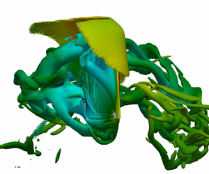
For high Mach number cases (e.g.  $Ma=1.4$), the major flow feature is the shock wave that is strongest in the midstroke. Figure 9 shows a top-down view of a rectangular wing at
  $Ma=1.4$ and
  $\alpha = 45^{\circ }$, in which a prevalent shock structure is present. It is observed that the spanwise flow of the LEV is heavily constrained as the spanwise flow inertia within the LEV is not great enough to overcome the resultant pressure differential across the shock wave generated near the wing tip. In addition, a large pressure gradient is observed along the leading edge of the wing. This raises the average pressure across the LEV. Despite this, a negative pressure coefficient is retained towards the end of the LEV in the chordwise direction, albeit smaller in magnitude compared to the subsonic cases. The wing slows down during pitch reversal, allowing the shock wave to propagate away from the wing and dissipate. When this occurs, the spanwise flow and the low pressure of the LEV are slightly recovered. Due to the higher pressure along the leading edge as a result of the shock front, coupled with the constrained spanwise flow, a substantial lift decrease is observed when compared to the lower Mach number cases. In addition to the degradation of the LEV, the wing-tip vortex goes from being a prominent flow structure in the low Mach number case (figure 7), to a substantially weaker flow structure in the high Mach number case (figure 9), further contributing to the decreased lift coefficient.

Figure 9. Vortex structures for  $Re = 200$,
  $Ma = 1.4$ and
  $\alpha = 45^{\circ }$ through a wing stroke: (a)
  $t=T/8$, (b)
  $t=2T/8$ and (c)
  $t=3T/8$. The shock wave is visible in the midstroke in (b), and propagates from the wing in (c). The shock wave is visualised by the Laplacian of density (
 $\boldsymbol {\nabla } \boldsymbol {\cdot }\boldsymbol {\nabla }\rho$) and is contoured by pressure coefficient. This shock wave stifles the spanwise flow of the LEV as observed in (b,c) when compared to the subsonic case. There is also a noticeable pressure rise of the LEV due to the shock wave.
Similar flow structures and vortex/shock interactions are observed when the AoA, wing kinematics and wing planforms are varied (figure 10). However, the decay rate of the coefficient of lift is a maximum for the rectangular wings at  $\alpha = 45^{\circ }$ (figure 2). Thus it is clear that the shock wave generated near the wing tip has a more detrimental effect on the aerodynamic force for cases experiencing larger lift. This is due to two distinct reasons. The first reason is that the appearance of the shock wave increases the average pressure of the LEV, with the largest variation occurring at the wing tip where the shock structure initially forms and is strongest. As such, the shock structure has a less detrimental effect for the cases that have less reliance on the region of the LEV towards the wing tip, such as high AoA cases, or cases of wings with a high aspect ratio (such as the bumblebee wing). Since there is less pressure and aerodynamic force contribution from vortex structures around the wing tip, and this is the region where the shock structure has the greatest impact, a lower decay rate is observed. The second reason is that for low AoA cases, the increased speed of the wing results in faster formation of the LEV. This allows for the LEV to form quickly just after stroke reversal before the shock structure forms, resulting in an increase in pressure difference across the wing earlier in the stroke.

Figure 10. Vortex structures in the midstroke for  $Re = 200$,
  $Ma = 1.4$ and
  $\alpha = 45^{\circ }$ for different wing planforms and kinematics: (a) rectangular wing undergoing the first kinematics; (b) rectangular wing undergoing the second kinematics; and (c) bumblebee wing undergoing the first kinematics. For all cases, the spanwise flow within LEV is constrained when compared to the subsonic cases. There is also a noticeable pressure rise of the LEV due to the shock wave.
The lack of spanwise flow of the LEV and the large pressure increase along the leading edge of the wing results in a degradation of the lift coefficient. A reduction of up to 45 % in the lift coefficient is observed between the low Mach number cases ( $Ma < 0.6$) and highest considered Mach number cases (
 $Ma = 1.4$).
3.2.2. Reynolds number 2000
As discussed in § 3.2.1, the shock wave limits the spanwise flow that could affect the stability of the LEV. Such effects could be strengthened at higher Reynolds numbers (e.g.  $Re=2000$). To discuss this effect, figure 11 shows the vortex structures at three typical instants for
  $\alpha = 45^{\circ }$ at
  $Re=2000$ and
  $Ma = 0.4$, and figure 12 shows the vortex structures at
  $2T/4$ for a variety of AoA, wing kinematics and wing planform cases. As shown in figure 11, the spanwise flow within the LEV and its stable attachment throughout the stroke for
  $\alpha = 45^{\circ }$ are similar to those at
  $Re=200$. The main difference between the two Reynolds number regimes is that the slight breakdown of the LEV near the wing tip is observed towards the end of the stroke for
  $Re=2000$. This has previously been observed for high Reynolds number flapping-wing cases (see e.g. Birch et al. Reference Birch, Dickson and Dickinson2004; Harbig et al. Reference Harbig, Sheridan and Thompson2013). When comparing this to higher AoA cases (such as
  $\alpha = 60^{\circ }$) at
  $Re = 2000$, the LEV exhibits increased instability towards the wing tip (as shown in figure 12).

Figure 11. Vortex structures for  $Re = 2000$,
  $Ma = 0.4$ and
  $\alpha = 45^{\circ }$ through the forward stroke: (a)
  $t=T/8$, (b)
  $t=2T/8$ and (c)
  $t=3T/8$.

Figure 12. Vortex structures for  $Re=2000$ and
  $Ma =0.4$ at
  $2T/4$ (midstroke) for a variety of cases and their associated wing pressure distribution: (a)
  $\alpha = 30^{\circ }$, (b)
  $\alpha = 45^{\circ }$, (c)
  $\alpha = 60^{\circ }$, (d)
  $\alpha = 45^{\circ }$ (second kinematics), and (e)
  $\alpha = 45^{\circ }$ (BB).
Figure 13 shows the vortex structures and shock wave at three typical instants for  $Re = 2000$,
  $Ma = 1.4$ and
  $\alpha = 45^{\circ }$. Figure 14 shows a top-down view of different wing planforms and wing kinematics without the shock wave to clearly visualise the LEV behaviours. At high Mach numbers (e.g.
  $Ma=1.4$), a significant difference in the flow structures is observed for the high Reynolds number cases when compared to the low Reynolds number cases. At approximately half the span length for the rectangular wing cases, and approximately one-quarter of the span length for the bumblebee wing planform, the LEV separates into two distinct vortex structures when a shock structure is present (figure 14). This is likely due to the higher spanwise velocity and inertia of the LEV when compared to lower Reynolds number flows. The second LEV structure reattaches to the wing tip or wing-tip vortex. The first LEV structure decays in a way similar to that of the LEV in the low Reynolds number case. A large pressure is once again observed along the leading edge, impacting the first LEV. This decreases the lift coefficient due to the average increase in the pressure of the LEV, in a way similar to that of the low Reynolds number case. The secondary vortex structure, however, retains a low pressure core, and its presence over the wing projects a negative pressure onto the top of the wing, resulting in some recovery of the decayed aerodynamic force, explaining why a smaller rate of decay in the lift coefficient is observed for higher Reynolds numbers, as demonstrated in figure 2.

Figure 13. Vortex structures and shock waves at three typical instants for  $Re = 2000$,
  $Ma = 1.4$ and
  $\alpha = 45^{\circ }$: (a)
  $t=T/8$, (b)
  $t=2T/8$ and (c)
  $t=3T/8$. The shock wave is visualised by the Laplacian of density (
 $\boldsymbol {\nabla }\boldsymbol {\cdot } \boldsymbol {\nabla } \rho$) and is contoured by the density gradient magnitude. The shock structures are shown as the concave structures around the wing tip. The shock generation in the midstroke, and its propagation and dissipation as the wing translates throughout the stroke, are the same as for the low Reynolds number case.

Figure 14. Each column corresponds to a different test case, each at  $Re = 2000$ and
  $Ma = 1.4$: (a) rectangular wing (
 $\alpha = 45^{\circ }$), (b) bumblebee wing (
 $\alpha = 45^{\circ }$), and (c) rectangular wing (
 $\alpha = 45^{\circ }$, 2nd kinematics). From top to bottom, for each case, the top-down views of vortex structures at four typical instants are considered (
 $T/8$,
  $2T/8$,
  $3T/8$ and
  $4T/8$). The shock structures have been removed from this figure to clearly observe the LEV. It can be seen that for each of these cases, the LEV splits into two distinct vortex structures at
  $2T/8$. This split occurs at approximately half the span length for the rectangular cases (a,c), and approximately one-quarter of the span length for the bumblebee case (b). At
  $3T/8$, partial recovery of the LEV is observed, while the LEV is fully recovered as the wing slows to subsonic speeds at
  $4T/8$.
Similar flow structures are observed for all cases considered in this study at  $Re=2000$ and
  $Ma=1.4$ (see figure 14), indicating the consistent flow physics, despite the variations in AoA, wing planform and kinematics. Once again, a smaller decay rate of the lift coefficient at higher AoA is observed as there is less contribution from the LEV near the wing tip to the aerodynamic lift when compared to lower AoA.
4. Scaling analysis
Lee et al. (Reference Lee, Choi and Kim2015) proposed a scaling law for hovering insects in incompressible flows through dimensional analysis based on real insect data. Based on the work by Lee et al. (Reference Lee, Choi and Kim2015), a correction factor is developed to account for compressibility and viscous effects to aid in engineering design and development for flapping-wing technology in highly compressible environments, such as Mars or very high altitudes on Earth. First, an approach similar to that of Lee et al. (Reference Lee, Choi and Kim2015) is used, with the LEV strength as a basis for aerodynamic force generation. Lee et al. (Reference Lee, Choi and Kim2015) stated that the strength of the LEV is scaled via circulation around the wing according to
 \begin{equation} \tau \sim \frac{U\bar{c}\varLambda\sin(\alpha)}{\varLambda+2}, \end{equation}
where  $\tau$ is the LEV strength,
  $U$ is the average wing tip velocity,
  $\bar {c}$ is the average chord length,
  $\varLambda$ is the aspect ratio, and
  $\alpha$ is the AoA of the wing. Following this, we can derive the reaction force (
 $F$) exerting on the wing as the changing rate of the vortical impulse (
 $I$) according to
 \begin{equation} F \sim \frac{\Delta I}{T} \sim \frac{\rho_\infty \tau R\bar{c}}{T}, \end{equation}
where  $\rho _\infty$ is the fluid density,
  $R$ is the span of the wing, and
  $T$ is the flapping period. In this study, the flapping period is defined as
 \begin{equation} T = \frac{2A_\phi(R + 0.1\bar{c})}{U}. \end{equation}
Substituting the flapping period (4.3) and the LEV strength (4.1) into the scaled force equation (4.2) results in
 \begin{equation} F \sim \frac{\rho_\infty R\bar{c}^2U^2\varLambda\sin(\alpha)}{2A_\phi(R + 0.1c)(\varLambda+2)}. \end{equation}
Recall that the force coefficient is defined as
 \begin{equation} C_F = \frac{2F}{\rho_\infty U^2 A}. \end{equation}
Since this is the total force coefficient, the vertical component (scaled coefficient of lift) is obtained by multiplying (4.5) by  $\cos (\alpha )$. Finally, combining this result with (4.4) yields the lift coefficient in terms of the flapping wing kinematics and geometric parameters:
 \begin{equation} C_L \sim \frac{\bar{c}\varLambda\sin(2\alpha)}{2A_\phi(R+0.1\bar{c})(\varLambda+2)}. \end{equation}
 In the results presented in figure 2, little variance with Mach number is observed in the global subsonic regime. However, there is a variation in  $C_L$ between different Reynolds numbers that is ignored in the previously derived equation. This variation of
  $C_L$ for different Reynolds numbers can be attributed to viscous forces that are not considered in the derived
  $C_L$ equation above. To account for this, the coefficient of lift can be separated into two distinct terms:
 \begin{equation} C_L = C_{LP} + C_{LV}, \end{equation}
where  $C_{LP}$ is the pressure contribution equivalent to
  $C_L$ in (4.6), and
  $C_{LV}$ is the viscous contribution to the dimensionless lift. Since (4.6) considers only the LEV, which is the pressure contribution of
  $C_L$, an additional viscous correction term must be added. This viscous correction term can be based on the work of Senturk & Smits (Reference Senturk and Smits2019) in the scaling law for the propulsive performance of a pitching aerofoil, where they observed a force coefficient dependency on the Reynolds number (
 $1/\sqrt {Re}$). By multiplying this by the normalised projected area of the wing (
 $({R\bar {c}}/{{c}^2})\sin (\alpha )$) relative to the direction of motion, an initial viscous correction factor (and coefficient of lift) can be defined as
 \begin{equation} \left.\begin{gathered} C_{LV} \sim{-}\frac{\varLambda\sin(\alpha)}{\sqrt{Re}}, \\ C_{L} \sim \frac{c\varLambda\sin(2\alpha)}{2A_\phi(R+0.1c)(\varLambda+2)} - \frac{\varLambda\sin(\alpha)}{\sqrt{Re}}. \end{gathered}\right\} \end{equation}
 This scaling law is valid when the wing is in the global subsonic regime. However, once the wing tip exceeds the speed of sound, the lift coefficient reduces with the increase of Mach number, and the reduction rate depends on both the Reynolds number and the AoA. Therefore, an additional correction factor is required for when shock structures are present. The decay of the lift coefficient with Mach number is approximately linear for all cases. This is different from the lift of stationary aerofoils in supersonic flows as predicted by the traditional theories (e.g. the linearised Ackeret and second-order Busemann theories; Cook Reference Cook2013). There are three potential reasons. First, supersonic flows occur only around the middle stroke, and subsonic and low speed flows occur at other stages (see figures 9 and 13). Second, the supersonic effect is effective only near the wing-tip region, as discussed in § 3.2. Third, here we consider only a limited range of Mach numbers (e.g. up to 1.4), thus the dependence of  $C_L$ on the Mach number may be linearised. Therefore, the correction factor takes the form
 \begin{equation} y = (mx\delta_c + b), \end{equation}
where  $y$ is the correction factor,
  $m$ is the rate of decay, and
  $\delta _c$ takes the value 1 when the wing is in the local supersonic regime, and 0 for the global subsonic regime. In this equation,
  $m$ is a function of Reynolds number and AoA, while
  $x$ is some Mach number value. The constant
  $b$ takes value 1 to ensure convergence to the globally subsonic solution for
  $C_L$ when
  $\delta _c = 0$.
The gradient of decay ( $m$) is effectively a weighting of the Reynolds number and AoA effect on the decay of
  $\overline {C_L}$. As observed by Chen et al. (Reference Chen, Wang, Zhou, Wu and Cheng2022), there is a limit in stable LEV intensity on revolving wings. Noting this Reynolds number effect, the gradient of decay can be mathematically defined as
 \begin{equation} m ={-}a/Re - b\sin(c\alpha). \end{equation}
 As the Reynolds number increases, the first term defining the decay rate trends to 0, implying the previously identified LEV intensity limit. Based on observations from data, the effects of the Reynolds number and AoA on decay rate at low Reynolds numbers are similar, while the AoA becomes the dominant factor when the Reynolds number increases to the LEV intensity limit. Since the greatest decay rate of the lift coefficient with increasing Mach number occurs at  $\alpha = 45^{\circ }$, and reduces similarly for lower and higher AoA, the coefficient
  $c$ is defined as
  $c = 2$. The coefficients
  $a$ and
  $b$ are scaling weights that will be added shortly, based on analysis of results. The
  $x$ value of the linear equation is a function of the Mach number, defined as the average Mach number of the wing tip, minus the critical average Mach number (when the wing tip becomes supersonic in the midstroke).
Based on these observations, the following scaling relationship is established:
 \begin{equation} C_{LP} \sim \frac{\bar{c}\varLambda\sin(2\alpha)}{2A_\phi(R+0.1\bar{c})(\varLambda+2)} \left[\left(\frac{1}{Re}-\sin(2\alpha)\right)(Ma - Ma_{crit})\delta_c+1\right]. \end{equation}
Using this scaled definition, applying weighted values for the scaled terms, considering the viscous force contribution and applying it to the vertical aerodynamic force, yields
 \begin{gather} L_P= \rho_\infty A_\phi R \bar{c}^2 f^2 (R+0.1\bar{c})\, \frac{\varLambda\sin(2\alpha)}{\varLambda+2} \left[\left(\frac{-40}{Re}-0.35\sin(2\alpha)\right)(Ma - Ma_{crit})\delta_c+1\right]. \end{gather}
Physically, this represents the lift force as a result of the LEV. The terms on the right-hand side of (4.12) before the square bracketed term are the geometric and kinematic parameter effects, while the square bracketed term represents the effects of compressibility on the LEV and total pressure lift.
The linear relationship of the above equation is shown in figure 15, where the pressure lift is taken as the total lift minus the viscous lift to facilitate the general aerodynamic force analysis. All numerical results follow this linear relationship at gradient 11.4, which is similar to the linear relationship identified by Lee et al. (Reference Lee, Choi and Kim2015), indicating that the scaling law derived in this paper holds for existing flapping-wing data, and provides a novel correction for flapping wings in highly compressible flows, providing a more general use of this scaling law for highly compressible environments.

Figure 15. Scaled lift relationship with compressibility corrections.
5. Conclusion
This paper presents a numerical study of the flow physics and aerodynamic performance of a three-dimensional hovering wing, focusing on the effects of compressibility and viscosity on the lift and subsequent scaling law. It is observed that the shock structures near the wing tip result in the limiting of the leading-edge vortex (LEV) spanwise flow. A degradation in the lift coefficient is observed due to this spanwise flow mitigation, coupled with the increase in average pressure of the LEV due to the shock front. At low Reynolds numbers, no lift coefficient recovery is observed for high Mach number cases, resulting in a high rate of decay with increasing shock strength. For high Reynolds numbers, a secondary LEV is identified that retains a low pressure core and is observed to reattach to either the wing tip or the wing-tip vortex. This results in some recovery of the lift coefficient. The rate of decay is observed to vary as a function of both Reynolds number and angle of attack. To quantify this change, a novel scaling law correction for the lift generation in highly compressible flows is proposed by considering the effects of compressibility and viscosity. This scaling law results in a linear relationship being observed between aerodynamic forces, LEV strength and its associated decay at high Mach numbers. Little deviation between the lift coefficient for constant Reynolds numbers when the wing is in the global subsonic flow regime is observed. Despite the decay in the lift coefficient with increasing Mach number, the increase in wing velocity still results in a higher lift achieved, indicating the ability of the flapping-wing flight mechanisms to maintain positive lift in highly compressible conditions. This study provides a basis for flapping wings in compressible flows inspired by the Martian atmospheric conditions.
This work is limited by the finite set of planforms, shapes and kinematics of wings. Further work is currently being undertaken to investigate additional factors that would impact the scaling law, such as wing shape, configuration, structural parameters and slip boundary conditions. While this study makes every effort to consider a wide variety of hovering flapping-wing cases, further studies are required to determine the optimal design for flapping wings in low-density environments, which will be considered in our future works.
Funding
This work was supported by the Australian Research Council (grant nos DP200101500 and DP240100294) and conducted with the assistance of computational resources from the National Computational Infrastructure, which is supported by the Australian Government.
Declaration of interests
The authors report no conflict of interest.
Appendix A. Validation of the solver – turbulence
In this appendix, the turbulence solver is validated by two cases for flow over a rigid sphere. This is due to the fact that the flow solver has two distinct sub-grid models as defined in the main paper. The first model is the Smagorinsky model to account for subgrid viscosity, and the second model accounts for turbulence compressibility effects and heat transfer. These models are validated independently to ensure that each model is accurate and cohesive.
The first case is a uniform flow over a sphere at Reynolds number 10 000 and Mach number 0.1 to test the Smagorinsky model without obvious compressibility. Table 1 shows the mean  $C_D$, the Strouhal number and the flow separation angle. It shows that the Strouhal number and separation angle have negligible variation when compared with the data obtained in the references. The coefficient of drag is within the range of presented by Constantinescu & Squires (Reference Constantinescu and Squires2004), and is within a deviation of 5 % compared with the results in the references.
Table 1. Validation study for flow over a rigid sphere at  $Re = 10\,000$ and
  $Ma = 0.1$ using the Smagorinsky model. In this table,
  $C_D$ is the drag coefficient,
  $St$ is the Strouhal number, and
  $\varphi_s$ is the flow separation angle from the sphere. The results of this study show good agreement with those in the literature.

The second case is a uniform flow over a rigid sphere at  $Re = 3700$ and
  $Ma = 0.6$, which is a well-studied case at the turbulent transition threshold. The Smagorinsky model is implemented alongside a thermal turbulence model defined in (2.8). The results of previous studies alongside this validation case are presented in table 2. This validation study provides excellent agreement with results published in the literature, with negligible deviation from those results presented by Rodríguez et al. (Reference Rodríguez, Lehmkuhl, Borrell and Oliva2013).
Table 2. Validation study for compressible flow over a rigid sphere at  $Re = 3700$ and
  $Ma = 0.6$. In this table,
  $C_D$ is the drag coefficient,
  $St$ is the Strouhal number, and
  $\varphi_s$ is the flow separation angle from the sphere. The results of this study show good agreement with those in the literature.

Finally, test cases for flapping wings (as considered in this study) are conducted with and without the LES model to ensure its accuracy and relevance. Figure 16 shows the lift coefficients for  $Re=2000$ and 6000. It is found that the difference in the forces predicted by the methods with and without LES is negligible, even at the highest Reynolds numbers considered. Based on the work by Lee et al. (Reference Lee, Kim and Kim2006), turbulence does not have a significant effect on the flapping foil in the uniform flow. Here, we further confirm that this conclusion applies to the flapping wing during hovering flight. This is because the flow considered is dominated by large, unsteady vortex structures. Turbulence would become more important for the cases involving acoustics or dynamics stall where the point of separation is sensitive to the viscosity.

Figure 16. Calculated lift force for (a)  $Re = 2000$ and (b)
  $Re = 6000$ with and without LES. Little force variation is observed, indicating that the LES model did not have significant effects on the results.
Figure 17 shows the vortical structures around the wing. It shows that the near-wing vortex structures are not significantly affected by the inclusion of LES. There is a variation in vortex structures further away from the wing as they break down, which is due to the nature of turbulence, but this does not have a significant effect on the force of the wing.

Figure 17. Vortex structures in the middle stroke for the case  $Re = 2000$,
  $Ma = 1.2$: (a) without LES and (b) with LES.
Appendix B. Validation of solver – transonic study
In this appendix, we consider the transonic cases  $Ma = 0.8$ and
  $0.95$ for a uniform flow over a rigid sphere at
  $Re = 300$, to ensure that the appropriate flow physics is captured in the transonic regime as it is a relevant regime for this study and can potentially result in numerical issues. This case is selected because it is numerically more challenging due to the sensitivity of the separation to the numerical set-up. The mean drag coefficient is shown in table 3, and the pressure coefficients around the sphere are shown in figure 18. It is found that our results show excellent agreement with the results by Nagata et al. (Reference Nagata, Nonomura, Takahashi and Fukuda2020). These successful validations, together with the fact that this solver has been used with success in previous studies involving transonic and supersonic flows, including prediction of force distribution along an aerofoil in transonic flows (Wang et al. Reference Wang, Tian and Liu2022b, Reference Wang, Young and Tian2024), provide confidence in its reliability in modelling the hovering wing considered in this work.
Table 3. Validation study for transonic flow over a rigid sphere at  $Re = 300$: the mean drag coefficients.


Figure 18. Validation study for a transonic flow over a sphere at  $Re = 300$: the pressure coefficients around the sphere.
Appendix C. Mesh convergence study
In this appendix, a mesh convergence study is conducted to ensure that the results reported in this work are independent of mesh at reasonable computational costs. For this mesh convergence study, two cases are considered. The first case is a hovering wing at  $Re = 200$,
  $Ma = 0.8$ (supersonic wing tip) and
  $\alpha = 60^{\circ }$ without a turbulence model, and the second case is a hovering wing at
  $Re = 2000$,
  $Ma = 0.8$ and
  $\alpha = 60^{\circ }$ with a compressible turbulence model. In this study, a non-uniform mesh is used. The grid is uniform in all three directions within an inner box
  $3\bar {c} \times 4.5\bar {c} \times 3\bar {c}$ where the wing motion occurs. The grid then gradually becomes coarser towards the outer boundaries where high flow structure resolution is not required for analysis of this problem, thereby reducing the computational cost. The uniform mesh region around the wing provides the basis for this mesh convergence study and is the location where the mesh size is varied. Mesh sizes
  $\Delta x = 0.08\bar {c}$,
  $0.04\bar {c}$ and
  $0.02\bar {c}$ are tested.
Figure 19 shows the lift coefficients for cases  $Re = 200$ and
  $2000$. For
  $Re=200$, mesh size
  $\Delta x = 0.08\bar {c}$ results in a 10 % offset in average lift coefficient when compared to
  $\Delta x = 0.02\bar {c}$, while there is a 3 % variation in
  $C_L$ between mesh sizes
  $\Delta x = 0.04\bar {c}$ and
  $0.02\bar {c}$. For
  $Re=2000$, mesh size
  $\Delta x = 0.08\bar {c}$ provides an approximately 3 % error in average lift coefficient when compared to
  $\Delta x = 0.02\bar {c}$, while there is negligible difference between mesh sizes
  $\Delta x = 0.04\bar {c}$ and
  $0.02\bar {c}$. Due to the computational resources required, coupled with the observation that there is minimal variation between
  $\Delta x = 0.04\bar {c}$ and
  $0.02\bar {c}$ for
  $Re = 2000$ (and an acceptable variation of 3 % for
  $Re = 200$), it was deemed unnecessary to reduce the mesh further.

Figure 19. Lift coefficient for (a)  $Re = 200$ and (b)
  $Re = 2000$, at
  $Ma = 0.8$ and
  $\alpha = 60^{\circ }$ at various mesh resolutions.
Based on these observations, mesh size  $\Delta x = 0.02\bar {c}$ is utilised for this study to ensure accuracy and consistency across all cases. This higher resolution mesh ensures that the shock interface is captured with a reasonable degree of clarity for flow field analysis.
Appendix D. Critical Mach number analysis
The effects of wing geometry and kinematic parameter on the critical Mach number are discussed. The wing geometry is defined by a general beta distribution function ( $B(p,q)$) as detailed by Ellington (Reference Ellington1984), in which the general shape of the majority of insect wings could be defined. According to this model, the wing shapes are defined by
 $$\begin{gather} \overline{r_1} = \int_0^1 \bar{c} \, \bar{r}\,{\rm d}\bar{r},\quad \overline{r_2} = 0.929\,\overline{r_1}^{0.732}, \end{gather}$$
 $$\begin{gather}p = \overline{r_1} \left(\frac{\overline{r_1}(1-\overline{r_1})}{\overline{r_2}^2 - \overline{r_1}^2} - 1 \right),\quad q = (1 - \overline{r_1}) \left(\frac{\overline{r_1}(1-\overline{r_1})}{\overline{r_2}^2 - \overline{r_1}^2} - 1 \right), \end{gather}$$
 $$\begin{gather}B(p,q) = \int_0^1 \bar{r}^{p-1} (1-\bar{r})^{q-1}\,{\rm d}\bar{r},\quad \bar{c} = \frac{\bar{r}^{p-1}(1-\bar{r}^{q-1}}{B(p,q)}, \end{gather}$$
where  $\bar {c}$ and
  $\bar {r}$ are respectively the chord length (normalised by the mean chord) and distance from the wing root in the spanwise direction (normalised by the wingspan), and
  $\overline {r_1}$ and
  $\overline {r_2}$ are the non-dimensional radii of first and second moments of area. Here, the same wing profiles as depicted by Shahzad et al. (Reference Shahzad, Tian, Young and Lai2016) are used. The values of
  $\overline {r_1}$ range from
  $0.43$ to
  $0.63$, and the aspect ratio
  $\varLambda$ ranges from
  $1.5$ to
  $6$. Finally, the midstroke pitching angles (
 $\theta$) ranging from
  $30^{\circ }$ to
  $60^{\circ }$ are considered.
Figure 20 shows the critical Mach number for wings of varying geometries and aspect ratios. While there is clearly an effect of wing geometry and motion on the critical Mach number, the wing profiles (excluding the extreme cases of high  $r_1$ and low aspect ratio) investigated here are close to
  $0.6$. The average critical Mach number of the rectangular wing is
  $Ma_{crit} = 0.62$. It ranges from 0.5 to 0.7 for all wings considered.

Figure 20. Critical Mach number analysis of various wing geometries and aspect ratios: (a) effect of wing geometry on Mach number; (b) critical Mach number as a function of  $\theta$.
Due to the large variable space of flapping-wing problems, and noting the limited availability of computational resources required to run these simulations, not all these wing geometries are considered here. However, based on the range of critical Mach numbers identified, generic rectangular and bumblebee wings provide a sufficient approximation of general flapping-wing aerodynamics for this study.


