


1. Introduction
In Natural Language Processing (NLP) tasks, text is either received as input or generated as output (e.g. machine translation, language modeling). In order to process text, it is common for neural networks applied to NLP tasks to split the original character string into a sequence of substrings, and to represent each substring as a discrete token. The granularity used to split the original text into substrings is part of the design of any NLP system.
Languages themselves offer information packaged at different natural granularity levels: sub-character information (e.g. radicals in Chinese characters), characters, morphemes, words, multi-word expressions, sentences and documents. Apart from the linguistically natural information packages, it is also possible to build synthetic partitions (e.g. statistically-discovered subwords Sennrich, Haddow, and Birch Reference Sennrich, Haddow and Birch2016, byte-level representations Costa-jussà, Escolano, and Fonollosa Reference Costa-jussà, Escolano and Fonollosa2017) as well as hybrid granularity levels (e.g. hybrid word-character representations Luong and Manning Reference Luong and Manning2016).
The representation granularity defines how to split a piece of text into a sequence of discrete tokens and is a key design aspect in any NLP system because it determines the type of information it can directly profit from. This way, a word-level system can profit from word-level information (e.g. semantics), while a character-level system does not have direct access to such a type of information.
The set of all possible tokens is referred to as vocabulary and, normally, the higher the representation granularity, the larger the size of the vocabulary. This way, the set of all possible words is larger than the set of all possible characters. Nevertheless, given the open nature of language, any finite size word-level vocabulary is to face the problem of words that are not part of the vocabulary and hence cannot be properly represented.
The selection of an appropriate granularity level is also influenced by the capability of the downstream NLP system to handle the resulting vocabulary. This way, while symbolic systems can handle very large vocabularies (i.e. several hundred thousand different tokens), current neural networks can only handle moderately large vocabularies (i.e. tens of thousand different tokens). This makes it desirable for Neural network-based NLP systems to keep the vocabulary size constrained while trying to maximize the representation ability.
The vocabulary is defined prior to the training of the neural network, normally by means of an algorithmic approach that “extracts” the possible tokens from the training data according to the chosen token granularity.
Character-level vocabularies define a token for each different character present in the training data. Their size ranges from tens to thousands of characters, depending on the language. In English, this would include all letters, both lowercase and uppercase, punctuation symbols, blanks, etc. A character-level vocabulary allows representing any text that contains the characters from the vocabulary, not only the words from the training data.
Word-level vocabularies define a token for each different word present in the training data. Given the huge amount of different words, only the N most frequent words are kept in the vocabulary, dropping the less frequent ones. The selection of hyperparameter N is driven by different factors, including hardware memory constraints, scaling limitations of the network architecture (e.g. softmax for network output) and the scarceness of lower frequency words in the training data (it is not useful to represent words whose frequency of appearance in the training data is not enough for the network to learn how to use them). A frequent default value is
 $N=32$
K tokens. A special token <UNK> is usually introduced in the vocabulary in order to represent words that are not part of the vocabulary (i.e. unknown words, or out-of-vocabulary (OOV) words).
$N=32$
K tokens. A special token <UNK> is usually introduced in the vocabulary in order to represent words that are not part of the vocabulary (i.e. unknown words, or out-of-vocabulary (OOV) words).
Multi-word level vocabularies extend word-based ones and try to find sequences of words that form a single lexical unit or are part of an idiomatic construct (Mikolov et al. Reference Mikolov, Sutskever, Chen, Corrado and Dean2013).
Subword vocabularies (Mikolov et al. Reference Mikolov, Sutskever, Deoras, Le, Kombrink and Cernocky2012) have word pieces as tokens, which are extracted statistically from the training data based on their frequency of appearance. For languages with regular morphology, extracted subwords may match morphological word parts, however, there is no guarantee of morphological soundness. Subword vocabularies normally do not have an <UNK> token because, apart from the multi-character subwords, there are usually single-character subwords that allow to represent any input text.
Despite their flexibility, character-level vocabularies delegate the learning of word formation to the network and the resulting token sequences are very long, which, for some tasks like machine translation (MT), leads to a decrease in the quality due to the model’s inability to handle long-range dependencies. On the other hand, word-level vocabularies relieve the network completely from learning word formation, but they frequently lead to OOV words and they aren’t aware of the connection of different forms of the same word, leading to worse training data utilization, especially for highly inflected languages and agglutinative languages. Subword vocabularies are a compromise between both, and are indeed used in the current state of the art of several NLP tasks, like MT.
Nevertheless, an asset of word-level vocabularies is that tokens can be associated with the word they represent, which can be key to certain tasks related to the meaning of the word or setups related to the word-level granularity (reuse of pretrained word embeddings for sentiment classification, induction of cross-lingual word embeddings); character and subword vocabularies lack such a trait and this makes them less suitable for such tasks.
1.1 Contribution
In this work, we propose the use of linguistic information to create vocabularies with the advantages of word-level and multiword-level representations and the flexibility of subword-level tokens. This work is in the line of recent efforts by the scientific communityFootnote a since our work focuses on the interpretability of the subword units that our NMT systems are using while profiting from the linguistic information available.
1.2 Manuscript organisation
In Section 2 we provide a review of the works in the area of incorporating linguistic information into neural NLP systems, especially for NMT. In Section 3 we describe in detail our proposed approach, while in Section 4 we describe the experimental setup used to evaluate it and explore the obtained results, followed by the discussion in Section 5. Finally, in Section 6 we draw the conclusions of this work. Appendix A provides information about the specific linguistic engine used as source for linguistic information used in this work and its relation to the proposed approach.
2. Related work
The first subword-based vocabularies were introduced by Schütze (Reference Schütze1993), while their first successful application to neural systems was with Byte-Pair Encoding (BPE) (Sennrich et al. Reference Sennrich, Haddow and Birch2016). This approach consists in taking all words from the training data and building subwords starting from a character-based vocabulary (with all characters present in the training data) and creating new tokens by iteractively merging the two tokens that appear together most frequently. BPE and some of its variants, such as word pieces (Wu et al. Reference Wu, Schuster, Chen, Le, Norouzi, Macherey, Krikun, Cao, Gao and Macherey2016), are the dominant subword vocabulary definition strategy in the state of the art neural machine translation (NMT) architectures.
Linguistic information was first introduced in a neural NLP system by Alexandrescu and Kirchhoff (Reference Alexandrescu and Kirchhoff2006), who proposed a language model (LM) where words are represented as a sequence of factors, that is, the word itself plus pieces of linguistic information associated with the word, like its POS tag or the its morphological characterization. Factors of different types are embedded in the same continuous space and the sequence of the previous
 $n-1$
embedded vectors is fed to the LM, which consists in a multilayer perceptron. The LM then generates the probability of the n-th token over the word space. In order to address the unknown word problem, they compute the average of all words belonging to the same POS tag; this way, if an unknown noun is to be fed to the network, all noun vectors in the embedded space would be averaged to compute the average noun vector.
$n-1$
embedded vectors is fed to the LM, which consists in a multilayer perceptron. The LM then generates the probability of the n-th token over the word space. In order to address the unknown word problem, they compute the average of all words belonging to the same POS tag; this way, if an unknown noun is to be fed to the network, all noun vectors in the embedded space would be averaged to compute the average noun vector.
Shaik et al. (Reference Shaik, Mousa, Schlüter and Ney2011) study different morphologically-grounded subword partition schemes applied to LM, including morpheme-based, syllable-based and grapheme-based, as well as their mix in the same vocabulary with word-based representations for the most frequent words. Vania and Lopez (Reference Vania and Lopez2017) study the effects of subword vocabularies in language models, including BPE and morphologically extracted subwords with Morfessor (Virpioja et al. Reference Virpioja, Smit, Grönroos and Kurimo2013). In their work, the predictions are normal words selected among the most frequent ones, but the input of the model are aggregations of subwords, either by mere addition or by means of biLSTMs.
The use of linguistic information was first introduced in NMT in the work by Sennrich and Haddow (Reference Sennrich and Haddow2016) (with precedents in SMT in the work by Ueffing and Ney Reference Ueffing and Ney2003 and Avramidis and Koehn Reference Avramidis and Koehn2008), who incorporate several linguistic features as input to the encoder of a standard sequence-to-sequence with attention model (Bahdanau, Cho, and Bengio Reference Bahdanau, Cho and Bengio2015). These features include the word’s lemma, POS tag and dependency type. The token granularity is subword level, making use of BPE to split low frequency words. Word-level features are copied to each of the subwords in the associated word. Both subword and linguistic features are encoded as discrete tokens from different representation spaces. Each token space is associated with a different embedded representation space, which a pre-defined dimensionality. At encoding time, the subword and the linguistic features are represented as their corresponding embedded vectors and then all vectors associated to a subword are concatenated together into the final representation.
Ponti et al. (Reference Ponti, Reichart and Korhonen2018) further refined the approach by Sennrich and Haddow (Reference Sennrich and Haddow2016) by injecting Universal Dependency tags (de Marneffe et al. Reference de Marneffe, Dozat, Silveira, Haverinen, Ginter, Nivre and Manning2014) as linguistic features and modifying the source analysis trees (e.g. by rearranging dependencies and introducing dummy nodes) to reduce the level of anisomorphism between source and target languages, directly affecting syntactic dependency tags. This improves translation quality, especially for typologically distant languages, as the linguistic information preprocessing reduces the gap between the structures of source and target languages.
In their work, Garcıa-Martınez et al. (Reference Garcıa-Martınez, Barrault and Bougares2016) proposed to modify the decoder part of a standard word-level sequence-to-sequence model to generate two elements per position of the output sentence: the first element is the lemma of the word, while the second element is the morphosyntactic information of the original word, which is referred to as factors. Each of the two outputs per position casts the probability over the lemma and factor space respectively. A similar approach was proposed by Song et al. (Reference Song, Zhang, Zhang and Luo2018) for the Russian language; they modify the decoder of a normal sequence-to-sequence with attention model to generate first the stem of the current word, and then its suffix based on the internal states and output of the decoder units, and then using a composite loss with separate terms for stems and for suffixes.
The generation of proper surface forms of morphologically rich languages has been studied in the literature, especially in transduction from morphologically simpler languages (e.g. English to German translation). With that purpose, Conforti et al. (Reference Conforti, Huck and Fraser2018) proposed to predict the morphological information of a morphologically rich language from merely the lemmas and word capitalization scheme.
Finally, Passban (Reference Passban2017) studies different word segmentation strategies and their influence over NMT translation quality. Some of the word segmentation approaches evaluated include leveraging Morfessor’s unsupervised morpheme discovery (Creutz and Lagus Reference Creutz and Lagus2002) and devising its own dynamic programming-based strategies.
3. Proposed approach
In this work we propose two different strategies that rely on linguistic information to provide morphologically sound vocabulary definitions for their use in neural networks applied to NMT.
In the following sections we describe both the vocabulary extraction phase and the token encoding phase for each of them, as illustrated in Figure 1. Note that the vocabulary extraction phase takes place before training the network and the token encoding phase takes place both at training time (to encode the training texts) and at inference time.
Figure 1. Vocabulary extraction and token encoding phases.
3.1 Morphological unit vocabulary
The goal of the Morphological Unit Vocabulary is to serve as a linguistically-grounded subword vocabulary. This vocabulary definition strategy relies on the morphological analysis of a sentence, which comprises a sequence of morphological units that may be lexical morphemes, multi-morpheme stems, separate inflectional morphemes or even fixed/semiflexible multi-word expressions, e.g. “in front of”.
During vocabulary extraction, all sentences in the training data are analyzed (see details about such an analysis in Appendix A) and their morphological units are used to elaborate the vocabulary, as shown in Figure 2. The specific information from the node that is incorporated as a token comprises the string associated with the node (being it a lexical morpheme, a word or a multi-word expression), together with its category, which is loosely analogous to the Part-of-Speech (POS) tag (e.g. noun stem (NST), verb stem(VST), noun flexion (N-FLEX)).

Figure 2. Morphological subword vocabulary extraction.
Figure 3. Token ID encoding process with the morphological unit vocabulary.
In order to encode a text into a sequence of tokens, the text is analyzed by means of a linguistic engine and the resulting morphological units are used as queries to find the associated token indexes from the vocabulary table, as shown in Figure 3.
Given the high amount of possible tokens and the practical size limitations of a vocabulary meant to be used with neural networks (described in Section 1), only the N most frequent tokens from the training data are selected to be part of the vocabulary.
If the analysis is driven by a lexicon, like in our case, this constrained vocabulary implies a mismatch with the unconstrained vocabulary used by the linguistic engine: when encoding the tokens of a text, the parse tree may contain terminal nodes that we cannot encode because they are not part of the vocabulary, either because they were not present in the training data or because their frequency of appearance was not enough to grant an entry in the final size-limited vocabulary. In order to eliminate such a vocabulary mismatch, once the Morphological Subword Vocabulary is extracted, the lexicon used by the linguistic engine (which drives the extraction of the morphological units) is pruned to remove any entry that is not part of the extracted vocabulary. These results in the removal of low-frequency words that, if encountered during the token encoding of a text, will be encoded as unknown words.
Words that are not part of the training data are marked in the analysis as unknown words. In order to cope with this OOV word situation, we can follow the approach by Luong and Manning (Reference Luong and Manning2016) and reserve some of the tokens in the vocabulary for character-based tokens. This way, any character found in the training data has its own token in the reserve character-based token range. As with subword vocabularies, this character-based subvocabulary makes <UNK> tokens not necessary for Mophologic Unit Vocabularies.
The resulting layout of the tokens table is outlined in Figure 4, with an initial range for special tokens like the end of sequence token or the padding token, an optional small range for character-level tokens, and finally the largest range for the morphological unit tokens.

Figure 4. Overall distribution of the morphological units vocabulary table.
Some examples of the resulting Mophological Unit tokenization are:
-
• The dogs are in the house: (the, DET), (dog, NST), (s, N-FLEX), (are, VST), (in, PREP), (the, DET), (house, NST),
 $\langle$
/s
$\rangle$
$\langle$
/s
$\rangle$
-
• My mom said I mustn’t tell lies: (my, DET), (mom, NST), (sai, VST), (d, V-FLEX), (I, PRN), (must, VST), (n’t, ADV), (tell, VST), (lie, NST), (s, N-FLEX)
$\langle$
/s
$\rangle$


3.2 Lemmatized vocabulary
The goal of the Lemmatized Vocabulary is to decouple meaning from morphological information in each word. For this, each word generates two tokens: one for the lemma and one for the relevant morphological traits of the word (e.g. gender, number, tense, case).
The source of linguistic information in this case is the morphosyntactic analysis of the sentence, which provides information for each word about its POS tag and its morphological features, such as gender, number, person, tense, case, etc. The presence of these features is language-dependent (e.g. some languages lack case or gender). Note that the morphological features do not contain information about the semantics of the word, but only about the morphological traits that, when added to the lemma, conform the specific surface form of the word.
During the vocabulary extraction phase, all sentences in the training data are analyzed and the resulting lemmas and morphological features are used to elaborate the vocabulary, as shown in Figure 5. For each word, the lemma is added to a lemma frequency counter, and the morphological features are added to an analogous morphological feature-set frequency counter.

Figure 5. Lemmatized Vocabulary extraction.
In order to encode a text into a sequence of tokens, the text is analyzed by means of the linguistic engine (see details about such an analysis in Appendix A). For each word, we obtain the lemma and the set of its morphological features (e.g. verb in present tense first person singular). For each lemma and for each morphological feature set we then query the vocabulary table for the appropriate token ID. This is illustrated in Figure 6, where the reuse of morphological feature set token IDs is highlighted in bold font.

Figure 6. Token encoding phase with the lemmatized vocabulary.
As in the Morphological Unit Vocabulary (see Section 3.1), the mismatch between the Lemmatized Vocabulary and the lexicon used for the morphosyntactic analysis is solved by pruning the latter to only contain elements from the former. The same way, unknown words are encoded by allocating a range of the token indexes for character-based tokens and using such character-based subvocabulary to encode any string that is marked as unknown. The distribution of the different elements present in a Lemmatized Vocabulary is illustrated in Figure 7.

Figure 7. Overall distribution of the lemmatized vocabulary table.
In order to cope with out-of-vocabulary words, we can reserve a range of tokens for character-level tokens so that any word or numeral can be encoded whether it was seen or not in the training data. The layout of the Lemmatized Vocabulary table is outlined in Figure 7, where we can see an initial range for special tokens, an optional range for character-based tokens, the largest range for the lemma tokens and the final range for every possible morphological feature set found in the training data. Note that another possibility to address the OOV words is to add the special token <UNK> to represent them and have a post-processing step to handle such a token; a frequent approach is to use the attention vector of sequence-to-sequence models to replace any <UNK> token at the output with the word from the input sentence with the highest attention value.
The nature of the linguistic engine we use gives us a morphosyntactic analysis with some deviations from the original sentence: first, the words in the sentence are rearranged to make turn its structure into a projective parse, if it was not projective already. This way, the English sentence “Who do you want me to talk to?” is rearranged as “You do want me to talk to who?”. A similar rearrangement occurs for other cases like separable phrasal verbs, which are rearranged so that the preposition sits next to the verb, and both form together a single multiword; this way “You let me down” would be rearranged into “You let down me”, and “let down” would be a single entity, with a single lemma and a single morphological feature set. This word rearrangements and aggregations favor a semantical interpretation of the sentence when used to represent the input to a neural system.
Given that the morphological information tokens always follow the lemma tokens, and that there are words in natural languages that do only admit one surface form, the lemmatized vocabulary can waste tokens that add no further information. In order to avoid such a situation, we only include the morphological information tokens if they are actually needed, that is, if the lemma they are associated to admits more than one surface form and hence can be subject to morphological variations.
Some examples of the resulting Lemmatized tokenization are:
-
• The dogs are in the house
lemma: the, morpho:(DET:(NU (PL SG))),
lemma: dog, morpho:(NST:(NU (PL) PS (3))),
lemma: be, morpho:(VST:(MD (IND) NU (PL) PF (FIN) PS (3)…)),
lemma: in, morpho:(PREP:()),
lemma: the, morpho:(DET:(NU (PL SG))),
lemma: house, morpho: (NST:(NU (SG) PS (3))),
$\langle$
/s
$\rangle$
-
• My mom said I mustn’t tell lies:
lemma: my, morpho: (DET:(NU (PL SG)),
lemma: mom, morpho: (NST:(NU (SG) PS (3)),
lemma: say, morpho: (VST:(MD (IND) NU (SG)…),
lemma: I, morpho: (PRN:(CA (S) NU (SG) PS (1))),
lemma: must, morpho:(VST:(MD (IND) NU (SG)…),
lemma: not,
lemma: tell, morpho:(VST:(MD (IND) NU (SG PL)…),
lemma: lie, morpho:(NST:(NU (PL) PS (3)),
$\langle$
/s
$\rangle$


4. Experiments
In order to evaluate the vocabulary definition strategies proposed in Section 3, we test them using machine translation as downstream task.
Table 1. Hyperparameters of the Transformer model for the NMT experiments
Neural Machine translation models compute the translation of a source sequence of tokens
 $x_1, \ldots, x_T$
by predicting token by token of the translation sequence
$x_1, \ldots, x_T$
by predicting token by token of the translation sequence
 $y_1,\ldots,y_{T'}$
, which has a potentially different length Tʹ:
$y_1,\ldots,y_{T'}$
, which has a potentially different length Tʹ:
 \begin{equation}p \left(y_1,\ldots,y_{T^{\prime}} | x_1, \ldots , x_T \right) = \prod _ {t=1}^{T^{\prime}} p \left(y_t| x, y_1, \ldots, y_{t-1} \right)\end{equation}
The currently dominant NMT architecture is the Transformer model (Vaswani et al. Reference Vaswani, Shazeer, Parmar, Uszkoreit, Jones, Gomez, Kaiser and Polosukhin2017), which surpasses in translation quality the original sequence to sequence models (Sutskever, Martens, and Hinton Reference Sutskever, Martens and Hinton2011; Cho et al. Reference Cho, van Merrienboer, Gulcehre, Bahdanau, Bougares, Schwenk and Bengio2014) and their variants with attention (Bahdanau et al. Reference Bahdanau, Cho and Bengio2015; Luong, Pham, and Manning Reference Luong, Pham and Manning2015). In our NMT experiments, we make use of the original implementation of the Transformer architecture by their authors, who released it as part of the tensor2tensor library. We use a standard configuration (transformer_base), with the hyperparameter configuration shown in Table 1, together with parameter averaging after convergence.
We performed experiments on English-German, French-English and Basque-Spanish datasets. The purpose of choosing those languages is to test the proposed vocabulary definition strategies both in morphologically rich languages (i.e. Basque, German) and in morphologically simpler ones (i.e. English).
German nouns are inflected for number (singular and plural), gender (masculine, feminine and neuter) and case (nominative, accusative, genitive and dative). French nouns are inflected for number (singular and plural) and gender (masculine and feminine). English nouns are only inflected for number (singular and plural) and case (nominative and genitive). Spanish nouns are inflected for number (singular and plural) and gender (masculine and feminine). Basque nouns are inflected (or rather they take suffixes for) number (singular, plural and “mugagabe”) and case (nominative, ergative, genitive, local genitive, dative, allative, inessive, partitive, etc.).
As far as verbs are concerned, German verbs have different inflections for 1st, 2nd and 3rd person singular and 1st/3rd persons and 2nd person plural in the present. French verbs are inflected for number and person, and gender in perfective compound tenses. English finite present tense verbal forms are only inflected in the 3rd person singular. Spanish verbs are inflected for person (1st, 2nd and 3rd), number (singular and plural), tense (present, past, future), aspect (perfective, punctual and progressive) and mood (indicative, subjunctive, conditional and imperative). Basque verbs take different forms for person (1st, 2nd and 3rd, not only for the subject but also for the direct and indirect objects), number (singular and plural), tense (present, past and future), aspect (progressive and perfect) and mood (indicative, subjunctive, conditional, potential and imperative).
Also, German presents compounds, that is, concatenation of words with no separation in between:
-
Übersetzungsqualität
$\rightarrow$
Übersetzung (translation) + s + Qualität (quality) -
Speicherverwaltung
$\rightarrow$
Speicher (memory) + Verwaltung (management)


For the English-German experiments, we make use of the WMT14 English-German news translation data.Footnote b The characteristics of the used training dataset are summarized in Table 2.
Table 2. Statistics of the German-English training data

For the French-English experiments, we make use of a combination of the News Commentary corpus and the Europarl corpus. The characteristics of the resulting training corpus are shown in Table 3
Table 3. Statistics of the French-English training data

For the Basque-Spanish experiments, we use the EiTB news corpus (Etchegoyhen, Azpeitia, and Pérez Reference Etchegoyhen, Azpeitia and Pérez2016). Its characteristics are shown in Table 4.
Table 4. Statistics of the Basque-Spanish training data

Table 5. German-English and English-German translation quality (case-insensitive BLEU score) with different source vocabulary strategies

*
 $p<0.05$
Table 6. French-English and English-French translation quality (case-insensitive BLEU score) with different source vocabulary strategies

*
 $p<0.05$
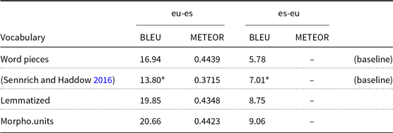
In order to evaluate the translation quality, we use BLEU (Papineni et al. Reference Papineni, Roukos, Ward and Zhu2002), which consists of an aggregation of n-gram matches together with a penalty for sentences shorter than the reference translations. The BLEU scores shown were computed by means of the sacrebleu tool (Post Reference Post2018) with the lower case setting. Given the known problems BLEU presents (Callison-Burch, Osborne, and Koehn Reference Callison-Burch, Osborne and Koehn2006), we also include the METEOR (Banerjee and Lavie Reference Banerjee and Lavie2005) scores, except for Basque, which is not supported by METEOR.
In Tables 5, 6 and 7 we can see the BLEU scores obtained by using different source vocabulary definition strategies, for German
 $\leftrightarrow$
English, English
$\leftrightarrow$
English, English
 $\leftrightarrow$
French and Basque
$\leftrightarrow$
French and Basque
 $\leftrightarrow$
Spanish respectively. As baselines, we used a word piece vocabulary (Wu et al. Reference Wu, Schuster, Chen, Le, Norouzi, Macherey, Krikun, Cao, Gao and Macherey2016) and the linguistic factored approach by Sennrich and Haddow (Reference Sennrich and Haddow2016). The word piece vocabulary was used for the original implementation of the Transformer model (Vaswani et al. Reference Vaswani, Shazeer, Parmar, Uszkoreit, Jones, Gomez, Kaiser and Polosukhin2017). The factored approach by Sennrich and Haddow (Reference Sennrich and Haddow2016) is the standard way for incorporating linguistic information; we used the same extra linguistic features as the authors, namely the lemma, POS tag and syntactic dependency label; as a subword vocabulary is used, each feature is copied to all subwords in the same word, and the position of the subword within the word (beginning, end, middle) is also added as feature; all feature embeddings are concatenated together with the token embedding to form the subword representation. In order to make this baseline comparable to the word piece baseline and to our own work, we added the linguistic features to the Transformer model instead of the original LSTM-based sequence-to-sequence with attention model from Sennrich and Haddow (Reference Sennrich and Haddow2016), keeping all the hyperparameters from the word piece baseline, while using the same linguistic feature-related hyperparamers from Sennrich and Haddow (Reference Sennrich and Haddow2016), namely the feature embedding dimensionalities.
$\leftrightarrow$
Spanish respectively. As baselines, we used a word piece vocabulary (Wu et al. Reference Wu, Schuster, Chen, Le, Norouzi, Macherey, Krikun, Cao, Gao and Macherey2016) and the linguistic factored approach by Sennrich and Haddow (Reference Sennrich and Haddow2016). The word piece vocabulary was used for the original implementation of the Transformer model (Vaswani et al. Reference Vaswani, Shazeer, Parmar, Uszkoreit, Jones, Gomez, Kaiser and Polosukhin2017). The factored approach by Sennrich and Haddow (Reference Sennrich and Haddow2016) is the standard way for incorporating linguistic information; we used the same extra linguistic features as the authors, namely the lemma, POS tag and syntactic dependency label; as a subword vocabulary is used, each feature is copied to all subwords in the same word, and the position of the subword within the word (beginning, end, middle) is also added as feature; all feature embeddings are concatenated together with the token embedding to form the subword representation. In order to make this baseline comparable to the word piece baseline and to our own work, we added the linguistic features to the Transformer model instead of the original LSTM-based sequence-to-sequence with attention model from Sennrich and Haddow (Reference Sennrich and Haddow2016), keeping all the hyperparameters from the word piece baseline, while using the same linguistic feature-related hyperparamers from Sennrich and Haddow (Reference Sennrich and Haddow2016), namely the feature embedding dimensionalities.
Table 7. Basque-Spanish and Spanish-Basque translation quality (case-insensitive BLEU score) with different source vocabulary strategies

*
 $p<0.05$
We used the implementation of the factored NMT Transformer from OpenNMT-py (Klein et al. Reference Klein, Kim, Deng, Senellart and Rush2017) with custom improvements in order to support specifying vocabulary sizes and embedding dimensions for the linguistic features. For the linguistic annotations we used Stanford’s corenlp (Manning et al. Reference Manning, Surdeanu, Bauer, Finkel, Bethard and McClosky2014) for English and French, ParZu (Sennrich et al. Reference Sennrich, Schneider, Volk and Warin2009; Sennrich, Volk, and Schneider Reference Sennrich, Volk and Schneider2013) for German, like in the original work by Sennrich and Haddow (Reference Sennrich and Haddow2016), LucyLT (Alonso and Thurmair Reference Alonso and Thurmair2003) for Basque and Spacy (Reference Honnibal and MontaniHonnibal and Montani to appear) for Spanish. Note that the Morphological Units and Lemmatized vocabularies include the character-level subvocabulary described in Section 3 to handle OOV words.
In all cases, the target language vocabulary strategy are word pieces in order to ensure a proper comparison.
As part of the experiments carried out, we also evaluate the influence of the proposed morphologically-based vocabularies on the translation quality for out of domain texts. For this, we use the WMT17 biomedical test sets, namely the English-German HimL test setFootnote c the French-German EDP test sets,Footnote d and a sample of 1000 sentences of the Open Data Euskadi IWSLT18 corpus (Jan et al. Reference Jan, Cattoni, Sebastian, Cettolo, Turchi and Federico2018), which contains documents from the Public Administration.
Given that these benchmarks are not included in sacrebleu, we used Moses’ multi-bleu.pl script, together with the standard tokenizer. The out-of-domain results are summarized in Tables 8, 9 and 10.
Table 8. German-English and English-German translation quality in out-of-domain text

*
 $p<0.05$
Table 9. French-English and English-French translation quality in out-of-domain text

*
 $p<0.05$
Table 10. Basque-Spanish and Spanish-Basque translation quality in out-of-domain text
*
 $p<0.05$
In order to assess the statistical significance of the differences between our proposed approaches and the word pieces baselines for the in-domain and out-of-domain test, we made use of the bootstrap resampling approach (Koehn Reference Koehn2004; Riezler and Maxwell Reference Riezler and Maxwell2005),Footnote e taking 95% as significance level (
 $p < 0.05$
). Statistical significance is reflected in the result tables with a * mark next to the BLEU score.
$p < 0.05$
). Statistical significance is reflected in the result tables with a * mark next to the BLEU score.
The obtained English
 $\leftrightarrow$
German results suggest that, while for the morphologically poor language (English) the translation quality is the same as the strong subwords baseline, the quality for the morphologically rich language (German) is improved in a statistically significant way. On the other hand, for English
$\leftrightarrow$
German results suggest that, while for the morphologically poor language (English) the translation quality is the same as the strong subwords baseline, the quality for the morphologically rich language (German) is improved in a statistically significant way. On the other hand, for English
 $\leftrightarrow$
French results are weaker in the case of the lemmatized vocabulary, while the morphological units vocabulary presents comparable performance to the word pieces baseline. For Basque and Spanish, we see a very large improvement of both lemmatized and morphological unit vocabulary, with to 3.5 BLEU points more than the word pieces baseline for Basque
$\leftrightarrow$
French results are weaker in the case of the lemmatized vocabulary, while the morphological units vocabulary presents comparable performance to the word pieces baseline. For Basque and Spanish, we see a very large improvement of both lemmatized and morphological unit vocabulary, with to 3.5 BLEU points more than the word pieces baseline for Basque
 $\rightarrow$
Spanish and 3.2 BLEU points for Spanish
$\rightarrow$
Spanish and 3.2 BLEU points for Spanish
 $\rightarrow$
Basque. We conclude that for the morphologically poor language, the use of linguistic vocabularies actually harms the translation quality for in-domain data, while for a morphologically rich language there is statistical evidence that the quality is higher than the strong subword baseline for out-of-domain data for German and comparable for French. This way, for the morphologically rich language with in-domain test data and for the morphologically poor language with out of domain data there is no statistical evidence to distinguish the quality of our proposed approaches from the strong subword baseline.
$\rightarrow$
Basque. We conclude that for the morphologically poor language, the use of linguistic vocabularies actually harms the translation quality for in-domain data, while for a morphologically rich language there is statistical evidence that the quality is higher than the strong subword baseline for out-of-domain data for German and comparable for French. This way, for the morphologically rich language with in-domain test data and for the morphologically poor language with out of domain data there is no statistical evidence to distinguish the quality of our proposed approaches from the strong subword baseline.
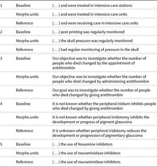
Table 11 shows some examples comparing the German-to-English outputs from out-of-domain text of the baseline and the Morphological Unit Vocabulary. The examples show that our linguistically-driven morphological segmentation has a clear impact on choosing more appropriate lexical units. Improvements come either from infrequent or specific words (e.g. glaucoma, irridotomy) or from generic words that are adequate for the particular context (e.g. units, administering).
Table 11. German-to-English out-of-domain examples
5. Discussion
The proposed linguistic knowledge-based vocabulary definition strategies offer a way to profit from morphosyntactic information for downstream tasks like MT. The two main differences with other approaches like factored NMT (Sennrich and Haddow Reference Sennrich and Haddow2016) derive from the use of a semantics-aware linguistic engine and from its non-aggregative management of linguistic information.
About the linguistic engine used, given that its ultimate goal is to perform rule-base translation, it needs to analyze the semantics of the input sentence, and uses it to disambiguate when multiple possible interpretations of a word are possible. When the disambiguation is not possible (e.g. when the subject of a sentence is not present and the verb conjugation admits more than one interpretation), the uncertainty is reflected in the analysis and our proposed vocabularies use such an information to compose the encoded representation. Another peculiarity of the used linguistic engine is that its analyses are driven by a lexicon. This makes it possible to adjust it to match the neural vocabulary in order to avoid mismatches between word and multi-word representations in both sides.
The non-aggregative encoding strategy makes it possible for the systems addressing the downstream tasks to directly use linguistic information, but also makes the resulting sequences longer. In order to further characterize the impact in sequence length, we computed the distribution of the ratio of the sequence lengths of both the Morphological Unit Vocabulary and the Lemmatized vocabulary with respect to a normal space and punctuation-based tokenization. The vocabularies are extracted from the training data, while the distribution is computed over a sample of 1000 sentences of the same dataset. We compute such a distribution for a configuration of our vocabularies where the OOV words are encoded as an <UNK> token and also where they are handled by a character-level subvocabulary, in order to understand the influence of this type of words over the final sequence length. The distribution of the same ratio for a word pieces vocabulary is also computed as reference. Figure 8 shows the distributions for the Morphological Unit Vocabulary, while Figure 9 shows it for the Lemmatized Vocabulary.

Figure 8. Distribution of the ratio of sequence length with the Morphological Unit Vocabulary and a standard word-based tokenization.

Figure 9. Distribution of the ratio of sequence length with the Lemmatized Vocabulary and a standard word-based tokenization.
As we can see in Figures 8 (Morphological Units) and 9 (Lemmatized), the sequence length with the proposed morphologically-grounded vocabularies with respect to the number of words in the sentence is higher than with word pieces (Wu et al. Reference Wu, Schuster, Chen, Le, Norouzi, Macherey, Krikun, Cao, Gao and Macherey2016), especially when the character-level subvocabulary is used to cope with the OOV words.
As shown in the figures, the differences in length depend on the morphological characteristics of the specific language. For English, with a simpler morphology, the ratio of sequence length with the proposed morphology-based vocabularies with respect to word pieces is higher than with German, French or Basque, which have richer morphology and hence needs also more word pieces for a single sentence.
This difference in length may affect the quality depending on the model’s ability to handle long-range dependencies. For instance, when multi-head attention mechanisms are known to be able to properly handle such type of dependencies, while RNNs present problems in that regard (Hochreiter Reference Hochreiter1991; Bengio, Simard, and Frasconi Reference Bengio, Simard and Frasconi1994).
The non-aggregative encoding strategy also allows using neural architectures without any modification, unlike the factored approaches like those by Sennrich and Haddow (Reference Sennrich and Haddow2016) and Garcıa-Martınez et al. (Reference Garcıa-Martınez, Barrault and Bougares2016), which need to account for the different representation spaces for lemmas and factors and keep separate embedding tables, which multiply the number of hyperparameters to tune, namely the vocabulary size and embedding dimensionality for each of the linguistic features. In this sense, the results obtained by factored approaches using the same hyperparameter configuration as Sennrich and Haddow (Reference Sennrich and Haddow2016) offer inferior translation quality compared to the word piece vocabulary; this can be attributed to the non optimality of the hyperparameters for our specific datasets and the usage of the Transformer architecture instead of the original LSTM sequence-to-sequence with attention model from Sennrich and Haddow (Reference Sennrich and Haddow2016).
Therefore, compared to word piece approaches and to the linguistic approach by Sennrich and Haddow (Reference Sennrich and Haddow2016), the mophological vocabularies approach is suitable for scenarios where the source language is a morphologically rich language like German, where the chosen neural architecture can handle long-range dependencies, like the Transformer model (in order to cope with the longer sequences), and where the available training data does not match the domain of the text the model is going to be fed as input at inference time.
6. Conclusion
Our experiments show that the proposed morphology-based vocabulary definition strategies provide improvements or maintain comparable quality in the translation of out-of-domain texts for languages that present a rich morphology like German and Basque. We also observe that no significant loss is suffered in translation quality for morphologically poor languages like English in that type of texts. Further work will consist of testing in other low-resourced NLP tasks which can benefit from more linguistic information.
Qualitatively, whenever we inject linguistic information in our neural systems, we are progressing in the interpretability of such systems. In this work we propose to do a linguistically-driven segmentation of our vocabulary, which enables morphologically-aware interpretation of the performance in downstream tasks. This is a line of research to be pursued in the future, especially in relation to the use of linguistic vocabularies for text generation, for instance, using the proposed vocabularies for the target side in NMT tasks.
Acknowledgements
This work is partially supported by Lucy Software/United Language Group (ULG) and the Catalan Agency for Management of University and Research Grants (AGAUR) through an Industrial PhD Grant. This work is also supported in part by the Spanish Ministerio de Economía y Competitividad, the European Regional Development Fund and the Agencia Estatal de Investigación, through the postdoctoral senior grant Ramón y Cajal, contract TEC2015-69266-P (MINECO/FEDER,EU) and contract PCIN-2017-079 (AEI/MINECO).
Appendix A. Rule-based machine translation as source for linguistic knowledge
In this work, we propose to make use of linguistic information to define vocabularies that confer certain desirable properties to the neural networks that use them.
There are multiple possible sources of linguistic information that could help define NMT vocabularies. Some options include using stemming algorithms, lemmatizers, POS-taggers and syntactic analyzers. While there exist several tools offering such capabilities, their availability is normally constrained to a single language, and their foundations are heterogeneous, including statistically-grounded, dictionary-based, or using machine learning approaches. In this work, we opt for the Rule-based Machine Translation (RBMT) Lucy LT system (Alonso and Thurmair Reference Alonso and Thurmair2003). This tool relies on knowledge distilled and formalized by human linguists in the form of lexicons and rules, and provides a consistent source of linguistic knowledge across several languages, including English, German, Spanish, French, Russian, Italian, Portuguese and Basque. Apart from translations, it provides linguistic analysis byproducts at different levels, which are used here as sources of linguistic information to devise the vocabularies proposed.
The Lucy RBMT system divides the translation process into three sequential stages: analysis, transfer and generation, as illustrated in Figure A1.
The analysis phase receives a sentence in the source language. After being tokenized, the sentence is morphologically analyzed, leveraging a monolingual lexicon to obtain all possible morphological readings of each word in the sentence. For instance, for the English word “works”, the two valid morphological readings are:
-
“work” (NST) + “s” (N-FLEX)
-
“work” (VST) + “s” (V-FLEX)
where NST stands for Noun Stem, N-FLEX for Nominal Inflectional Suffix, VST for Verb Stem and V-FLEX for Verbal Suffix.

Figure A1. Workflow of rule-based machine translation systems.
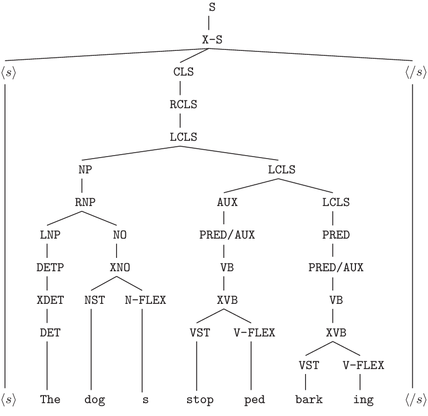
Figure A2. Parse tree for sentence “The dogs stopped barking”.
A chart parser together with an analysis grammar converts the sequence of valid morphological readings of the words comprising the sentence and outputs a parse tree. The terminal nodes of the parse tree (i.e. the leave nodes) depend on the monolingual lexicon used during the parse phase. Based on entries in such a lexicon, the parser tries to find inflectional and derivational constructions.
An example of parse tree is shown in Figure A2.
The terminal nodes of the parse tree are the source of the morphologic analysis used to create the Morphological Unit Vocabulary described in Section 3.1.
The parse tree is then applied a second set of rules that annotate, rearrange and mutate the original parse tree nodes, to output an analysis tree, which resembles a projective constituency tree (non projective constructs are rearranged into projective versions). In this tree, words are no longer separated into different nodes representing their morphological parts, but are assembled into a single node with features expressing its morphological traits (e.g. gender, number, verbal tense, person, case).
There is an extra post-processing sub-stage called mirification that performs the final retouches, outputting the MIR (Metal Interface RepresentationFootnote f) tree. An example of MIR tree is show in Figure A3. While there is a noticeable depth reduction in comparison with the parse tree for the same sentence shown in Figure A2, there are also other non-evident differences: flexions have been merged with their associated lemmas, and the morphological information has been condensed as node features, which are not show in these tree representations.

Figure A3. MIR tree for sentence “The dogs stopped barking”.
The whole analysis phase is only dependent on the source language and can therefore be reused for language pairs with the same source language. This phase relies in a monolingual lexicon that contains entries for words in the source language, together with metainformation that allows their inflection and morphological derivation. It also relies in an analysis grammar, that is, a set of declarative rules that are matched to the input tokens and structures and allow the iterative construction of the parse and analysis trees.
The terminal nodes (i.e. leaves) of the MIR tree are used as the source of the morphosyntactic analysis of the sentence used to create the Lemmatized Vocabulary described in Section 3.2. In the MIR tree, terminal nodes represent at least one word: during the analysis phase, any flexion node is merged with the main word node and such a node gets annotated with morphological features like gender, number, person, tense, case, etc. The presence of these features is language-dependent (e.g. some languages lack case or gender). The morphological features are disambiguated as much as possible taking information from other parts of the sentence (e.g. the person of a verbal form may be disambiguated by the sentence subject). Where not possible, the uncertainty is expressed (e.g. stating all the possible persons the verbal form can be in).
The Lucy analysis takes into account the presence of multi-word expressions (MWE) and handles them as a single element when they are included in the lexicon. This helps in capturing the semantics of such constructs during the translation process. This includes not only fixed MWEs (e.g. “in front of”), but also flexible MWEs. For instance, verbal constructions like “take into account” are identified and grouped into a single element.
In the transfer stage, the MIR tree is annotated and mutated into a transfer tree that is suitable as input for the generation phase. There are different types of transfer operations, such as language-pair dependent operations (e.g. mapping of idiomatic expressions), contextual transfer and lexical transfer.
The transfer stage is language-direction dependent. It relies on a bilingual lexicon that contains word and expression translations, together with their context-dependent applicability criteria. It also relies on a transfer grammar, that is, a set of imperative rules that implement the needed transformations and annotations.
The generation stage receives as input the transfer tree and generates the final translation, performing any needed reorderings and adaptations. This stage is only dependent on the target language (i.e. it can be reused for any source side language). It relies on a monolingual target language lexicon, together with a generation grammar, that is, a set of imperative rules to generate the output sentence.


