2. Geometry and governing equations

Let us consider an axisymmetric flow taking place in a cylindrical cavity of radius $R$ (see figure 1). As such, we focus exclusively on solutions that are invariant to rotations about the axis of the channel, i.e. $\partial _{{\it\theta}}=0$ . The domain is bounded by two no-slip horizontal walls located at $z=0$ and $z=h$ , and is filled with an electrically conducting fluid (typically a liquid metal such as Galinstan, of electrical conductivity ${\it\sigma}=3.4\times 10^{6}~\text{S}~\text{m}^{-1}$ , density ${\it\rho}=6400~\text{kg}~\text{m}^{-3}$ and viscosity ${\it\nu}=4\times 10^{-7}~\text{m}^{2}~\text{s}^{-1}$ ). A static and uniform magnetic field $B_{0}\,\boldsymbol{e}_{z}$ is applied vertically. The low-Rm approximation is assumed to hold, meaning that the magnetic field induced by the flow is negligible compared to the imposed magnetic field (Roberts Reference Roberts1967). Consequently, the total magnetic field $\boldsymbol{B}$ is uniform across the domain and follows $\boldsymbol{B}=B_{0}\,\boldsymbol{e}_{z}$ . In addition, the electric field $\boldsymbol{E}$ is derived from the electric potential ${\it\phi}$ according to $\boldsymbol{E}=-\boldsymbol{{\rm\nabla}}{\it\phi}$ . A flow is driven by injecting electric current through an electrode of radius ${\it\eta}$ located on the bottom plate. The top and bottom plates are perfectly electrically insulating otherwise, which forces the current to exit the channel through the sides. In anticipation of the upcoming calculations, the profile of injected current is assumed to be a smooth function, such as the Gaussian distribution:

(2.1) $$\begin{eqnarray}j_{z}^{w}(r)=\frac{I_{0}}{{\rm\pi}{\it\eta}^{2}}\exp \!\left[-(r/{\it\eta})^{2}\right],\end{eqnarray}$$

where $I_{0}$ is the total current injected inside the domain up to the correction factor $(1-\exp [-(R/{\it\eta})^{2}])$ , which is almost identical to 1 for $R/{\it\eta}>10$ . Given this configuration, the electric current is known to flow radially, interacting with the vertical magnetic field to induce a patch of vertical vorticity right above the bottom Hartmann layer.

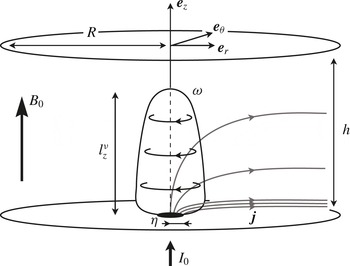
Figure 1. Sketch of the problem. An isolated vortex of height $l_{z}^{{\it\nu}}<h$ confined between two horizontal no-slip and electrically insulating walls a distance $h$ apart.

In the inertialess limit (Kalis & Kolesnikov Reference Kalis and Kolesnikov1980), the development of this patch of vorticity relies on the competition between two effects. On the one hand, the rotational part of the Lorentz force diffuses momentum along the magnetic field (Sommeria & Moreau Reference Sommeria and Moreau1982), hence leading to a vortex extending in the $z$ direction. On the other hand, viscous friction diffuses momentum isotropically, therefore opposing the growth of the vortex along $z$ . Calling $l_{z}^{{\it\nu}}$ the range of action of the Lorentz force, its diffusive effect takes place over the characteristic time ${\it\tau}_{2D}=({\it\rho}/{\it\sigma}B_{0}^{2})(l_{z}^{{\it\nu}}/{\it\eta})^{2}$ . Conversely, viscous dissipation takes place over the time ${\it\tau}_{{\it\nu}}={\it\eta}^{2}/{\it\nu}$ . Assuming a steady flow, the distance $l_{z}^{{\it\nu}}$ over which the Lorentz force is able to act before being balanced by viscous dissipation is derived by equating the two effects, yielding:

(2.2) $$\begin{eqnarray}\frac{l_{z}^{{\it\nu}}}{h}=\frac{{\it\eta}^{2}}{h^{2}}\,\mathit{Ha},\end{eqnarray}$$

where $\mathit{Ha}=B_{0}h\sqrt{{\it\sigma}/{\it\rho}{\it\nu}}$ is the Hartmann number based on the height of the channel. Asymptotically speaking, $l_{z}^{{\it\nu}}/h\ll 1$ means that the diffusive effect of the Lorentz force is balanced by viscous dissipation long before momentum can reach the top wall. In this case, the distance $l_{z}^{{\it\nu}}$ may be physically interpreted as the height of the vortex. In contrast, $l_{z}^{{\it\nu}}/h\gg 1$ means that momentum can be diffused far beyond the top wall. This process, however, is blocked by the presence of the no-slip top wall, which prevents the vortex from extending past it. The ratio $l_{z}^{{\it\nu}}/h$ has been identified by Pothérat & Klein (Reference Pothérat and Klein2014) as the non-dimensional parameter defining whether the structure is able to feel the presence of the top wall, hence controlling its dimensionality: 3D when $l_{z}^{{\it\nu}}/h\ll 1$ and quasi-2D when $l_{z}^{{\it\nu}}/h\gg 1$ .

From now on, let us use the dimensionless coordinates $\tilde{r}=r/{\it\eta}$ and $\tilde{z}=z/h$ , as well as the non-dimensional variables $\tilde{u} =u/U$ , $\tilde{{\it\omega}}={\it\omega}\,{\it\eta}/U$ , $\tilde{j}=j/{\it\sigma}UB_{0}$ and $\tilde{{\it\phi}}={\it\phi}/UB_{0}{\it\eta}$ . We also introduce the non-dimensional operator $\tilde{\boldsymbol{{\rm\nabla}}}$ defined as

(2.3) $$\begin{eqnarray}\tilde{\boldsymbol{{\rm\nabla}}}=\left(\frac{\partial }{\partial \tilde{r}},\frac{1}{\tilde{r}}\frac{\partial }{\partial {\it\theta}},\frac{{\it\eta}}{h}\frac{\partial }{\partial \tilde{z}}\right).\end{eqnarray}$$

The scaling for the velocity $U$ is derived from the linear theory of quasi-2D electrically driven vortices put forward by Sommeria (Reference Sommeria1988). It is estimated from $U=({\it\Gamma}/{\it\eta})\sqrt{l_{z}^{{\it\nu}}/h}$ , where ${\it\Gamma}=I_{0}/2{\rm\pi}\sqrt{{\it\sigma}{\it\rho}{\it\nu}}$ is the circulation induced right above a point-like electrode through which flows the current $I_{0}$ , when viscous friction in the horizontal plane is neglected. This scaling for $U$ is representative of the velocity at the edge of the vortex core, whose radius results from the competition between the Lorentz force and viscous dissipation. Hence the explicit dependence of $U$ on the ratio $l_{z}^{{\it\nu}}/h$ . The governing equations consist of the steady-state vorticity equation for $\tilde{{\bf\omega}}=\tilde{\boldsymbol{{\rm\nabla}}}\times \tilde{\boldsymbol{u}}$ ,

(2.4) $$\begin{eqnarray}\frac{1}{N}\left(\tilde{\boldsymbol{u}}\boldsymbol{\cdot }\tilde{\boldsymbol{{\rm\nabla}}}\tilde{{\bf\omega}}-\tilde{{\bf\omega}}\boldsymbol{\cdot }\tilde{\boldsymbol{{\rm\nabla}}}\tilde{\boldsymbol{u}}\right)=\frac{1}{\mathit{Ha}}\left(\frac{l_{z}^{{\it\nu}}}{h}\right)^{-1}\tilde{{\rm\Delta}}\tilde{{\bf\omega}}+\frac{1}{\sqrt{\mathit{Ha}}}\left(\frac{l_{z}^{{\it\nu}}}{h}\right)^{1/2}\frac{\partial \tilde{\boldsymbol{j}}}{\partial \tilde{z}},\end{eqnarray}$$

Ohm’s law

(2.5) $$\begin{eqnarray}\tilde{\boldsymbol{j}}=-\tilde{\boldsymbol{{\rm\nabla}}}\tilde{{\it\phi}}+\tilde{\boldsymbol{u}}\times \boldsymbol{e}_{z},\end{eqnarray}$$

the conservation of mass

(2.6) $$\begin{eqnarray}\tilde{\boldsymbol{{\rm\nabla}}}\boldsymbol{\cdot }\tilde{\boldsymbol{u}}=0\end{eqnarray}$$

and charge

(2.7) $$\begin{eqnarray}\tilde{\boldsymbol{{\rm\nabla}}}\boldsymbol{\cdot }\tilde{\boldsymbol{j}}=0.\end{eqnarray}$$

The problem at hand is governed by three non-dimensional parameters, namely the interaction parameter $N$ based on the width of the injection electrode ${\it\eta}$ , the Hartmann number $\mathit{Ha}$ based on the height of the channel $h$ and the ratio $l_{z}^{{\it\nu}}/h$ :

(2.8a−c ) $$\begin{eqnarray}N=\frac{{\it\sigma}B_{0}^{2}{\it\eta}}{{\it\rho}U},\quad \mathit{Ha}=B_{0}h\,\sqrt{\frac{{\it\sigma}}{{\it\rho}{\it\nu}}},\quad \frac{l_{z}^{{\it\nu}}}{h}=\frac{{\it\eta}^{2}}{h^{2}}\,\mathit{Ha}.\end{eqnarray}$$

The boundary conditions on the horizontal walls consist of no-slip boundaries

( i ) $$\begin{eqnarray}\tilde{\boldsymbol{u}}(\tilde{r},0)=\tilde{\boldsymbol{u}}(\tilde{r},1)=0,\end{eqnarray}$$

an imposed vertical current at the bottom wall

( i i ) $$\begin{eqnarray}\tilde{j}_{\tilde{z}}(\tilde{r},0)=\tilde{j}_{\tilde{z}}^{w}(\tilde{r})\end{eqnarray}$$

and a perfectly electrically insulating top wall

( i i i ) $$\begin{eqnarray}\tilde{j}_{\tilde{z}}(\tilde{r},1)=0.\end{eqnarray}$$

In addition, we impose a perfectly conducting and free-slip radial boundary

( i v ) $$\begin{eqnarray}\tilde{j}_{\tilde{z}}(\tilde{R},\tilde{z})=0\end{eqnarray}$$

and

( v ) $$\begin{eqnarray}\tilde{{\bf\tau}}_{\tilde{r}}(\tilde{R},\tilde{z})=0,\end{eqnarray}$$

where $\tilde{{\bf\tau}}_{\tilde{r}}$ represents the shear stress exerted on the wall whose normal vector is  $\boldsymbol{e}_{r}$ . These boundary conditions were chosen to match as closely as possible the experimental set-ups of Sommeria (Reference Sommeria1988) and Pothérat & Klein (Reference Pothérat and Klein2014), where a flow is driven by injecting a known amount of electric current $I_{0}$ . The free-slip and perfectly conducting radial boundary can be physically interpreted as a pseudo-wall made of liquid metal, and was preferred over a no-slip boundary condition as it does not introduce parallel layers along the radial boundary. Keeping the experimental analogy in mind, the model we propose here focuses on an elementary structure, which has been extracted from an array of vortices.

Considering the scaling that was chosen for $U$ , the normalized bottom boundary condition on the current $\tilde{j}_{z}^{w}$ is expressed as

(2.9) $$\begin{eqnarray}\tilde{j}_{\tilde{z}}^{w}(\tilde{r})=\frac{2}{\sqrt{\mathit{Ha}}}\left(\frac{l_{z}^{{\it\nu}}}{h}\right)^{-1}\exp \!\left(-\tilde{r}^{2}\right).\end{eqnarray}$$

In other words, for a given value of $\mathit{Ha}$ and $l_{z}^{{\it\nu}}/h$ , the intensity of the total injected current is adjusted so that the intensity of the resulting flow remains comparable throughout all cases investigated.

We shall now consider a weakly inertial flow in the limit $N\gg 1$ , and expand (2.4)–(2.7) using the regular perturbation series:

(2.10) $$\begin{eqnarray}\displaystyle & \tilde{\boldsymbol{j}}=\tilde{\boldsymbol{j}}^{_{0}}+N^{-1}\,\tilde{\boldsymbol{j}}^{_{1}}+N^{-2}\,\tilde{\boldsymbol{j}}^{_{2}}+O(N^{-3}), & \displaystyle\end{eqnarray}$$

(2.11) $$\begin{eqnarray}\displaystyle & \tilde{\boldsymbol{u}}=\tilde{\boldsymbol{u}}^{_{0}}+N^{-1}\,\tilde{\boldsymbol{u}}^{_{1}}+N^{-2}\,\tilde{\boldsymbol{u}}^{_{2}}+O(N^{-3}), & \displaystyle\end{eqnarray}$$

(2.12) $$\begin{eqnarray}\displaystyle & \tilde{{\bf\omega}}=\tilde{{\bf\omega}}^{_{0}}+N^{-1}\,\tilde{{\bf\omega}}^{_{1}}+N^{-2}\,\tilde{{\bf\omega}}^{_{2}}+O(N^{-3}). & \displaystyle\end{eqnarray}$$

3. Inertialess base flow

The equations governing the problem at leading order are

(3.1) $$\begin{eqnarray}\displaystyle & \displaystyle \tilde{{\rm\Delta}}\tilde{{\bf\omega}}^{_{0}}=-\sqrt{\mathit{Ha}}\,\left(\frac{l_{z}^{{\it\nu}}}{h}\right)^{3/2}~\frac{\partial \tilde{\boldsymbol{j}}^{_{0}}}{\partial \tilde{z}}, & \displaystyle\end{eqnarray}$$

(3.2) $$\begin{eqnarray}\displaystyle & \tilde{\boldsymbol{j}}^{_{0}}=-\tilde{\boldsymbol{{\rm\nabla}}}\tilde{{\it\phi}}^{_{0}}+\tilde{\boldsymbol{u}}^{_{0}}\times \boldsymbol{e}_{z}, & \displaystyle\end{eqnarray}$$

(3.3) $$\begin{eqnarray}\displaystyle & \tilde{\boldsymbol{{\rm\nabla}}}\boldsymbol{\cdot }\tilde{\boldsymbol{u}}^{_{0}}=0, & \displaystyle\end{eqnarray}$$

(3.4) $$\begin{eqnarray}\displaystyle & \tilde{\boldsymbol{{\rm\nabla}}}\boldsymbol{\cdot }\tilde{\boldsymbol{j}}^{_{0}}=0. & \displaystyle\end{eqnarray}$$

Solving $\tilde{{\bf\omega}}^{_{0}}$ and $\tilde{\boldsymbol{j}}^{_{0}}$ can be done separately by taking the Laplacian of the vorticity equation (2.4) on the one hand, and taking the Laplacian of twice the curl of Ohm’s law (2.5) on the other hand. Combining them yields the following set of equations:

(3.5) $$\begin{eqnarray}\tilde{{\rm\Delta}}^{2}\tilde{{\bf\omega}}^{_{0}}=\left(\frac{l_{z}^{{\it\nu}}}{h}\right)^{2}\frac{\partial ^{2}\tilde{{\bf\omega}}^{_{0}}}{\partial \tilde{z}^{2}}\end{eqnarray}$$

and

(3.6) $$\begin{eqnarray}\tilde{{\rm\Delta}}^{2}\tilde{\boldsymbol{j}}^{_{0}}=\left(\frac{l_{z}^{{\it\nu}}}{h}\right)^{2}\frac{\partial ^{2}\tilde{\boldsymbol{j}}^{_{0}}}{\partial \tilde{z}^{2}}.\end{eqnarray}$$

It is quite remarkable that (3.5) and (3.6) can be solved independently, and depend on the same and unique parameter $l_{z}^{{\it\nu}}/h$ . They remain nonetheless coupled via twice the curl of Ohm’s law:

(3.7) $$\begin{eqnarray}\tilde{{\rm\Delta}}\tilde{\boldsymbol{j}}^{_{0}}=-\frac{1}{\sqrt{\mathit{Ha}}}\left(\frac{l_{z}^{{\it\nu}}}{h}\right)^{1/2}\,\frac{\partial \tilde{{\bf\omega}}^{_{0}}}{\partial \tilde{z}}.\end{eqnarray}$$

Equations (3.5) and (3.6) admit a purely azimuthal solution for $\tilde{\boldsymbol{u}}^{_{0}}$ and a purely meridional solution for $\boldsymbol{j}^{_{0}}$ . Consequently, knowing either component $\tilde{{\it\omega}}_{\tilde{z}}^{_{0}}$ or $\tilde{{\it\omega}}_{\tilde{r}}^{_{0}}$ , and $\tilde{j}_{\tilde{r}}^{_{0}}$ or $\tilde{j}_{\tilde{z}}^{_{0}}$ is enough to completely derive the solution at leading order. The boundary conditions associated with the leading order read

( i ⁰ ) $$\begin{eqnarray}\tilde{{\it\omega}}_{\tilde{z}}^{_{0}}(\tilde{r},0)=\tilde{{\it\omega}}_{\tilde{z}}^{_{0}}(\tilde{r},1)=0,\end{eqnarray}$$

( i i ⁰ ) $$\begin{eqnarray}\tilde{j}_{\tilde{z}}^{_{0}}(\tilde{r},0)=\tilde{j}_{\tilde{z}}^{w}(\tilde{r}),\end{eqnarray}$$

( i i i ⁰ ) $$\begin{eqnarray}\tilde{j}_{\tilde{z}}^{_{0}}(\tilde{r},1)=0,\end{eqnarray}$$

( i v ⁰ ) $$\begin{eqnarray}\tilde{j}_{\tilde{z}}^{_{0}}(\tilde{R},\tilde{z})=0.\end{eqnarray}$$

In addition, we shall approximate boundary condition (v) by

( v ⁰ ) $$\begin{eqnarray}\tilde{{\it\omega}}_{\tilde{z}}^{_{0}}(\tilde{R},\tilde{z})=0.\end{eqnarray}$$

Boundary condition (v⁰ ) is not entirely equivalent to the free-slip boundary condition (v), which can be rewritten in terms of $\tilde{{\it\omega}}_{\tilde{z}}^{_{0}}$ as

(3.8) $$\begin{eqnarray}\tilde{{\it\omega}}_{\tilde{z}}^{_{0}}(\tilde{R},\tilde{z})=\frac{2}{\tilde{R}}~\tilde{u} _{{\it\theta}}^{_{0}}(\tilde{R},\tilde{z}).\end{eqnarray}$$

It is only in the limit $\tilde{R}\gg 1$ (since $\tilde{u} _{{\it\theta}}^{_{0}}$ is of order 1) that boundary condition (v) may be approximated by (v⁰ ). However, (v⁰ ) offers a much simpler numerical implementation. Indeed, not only does it remove any remaining dependency on $\tilde{u} _{{\it\theta}}^{_{0}}$ , it also naturally introduces an orthogonal basis of functions on which the solution can be projected. From a practical point of view, we ensured that the edge of the channel was sufficiently far from the injection area in order to minimize the impact of this approximation on the flow (see § 5).

Solutions with separated variables of (3.5) and (3.6), which satisfy the coupling (3.7), as well as boundary conditions (iv⁰ ) and (v⁰ ) are of the form

(3.9) $$\begin{eqnarray}\tilde{{\it\omega}}_{\tilde{z}}^{_{0}}=\mathop{\sum }_{n=1}^{\infty }\text{J}_{0}({\it\lambda}_{n}\,\tilde{r})~\mathop{\sum }_{i=1}^{4}A_{ni}\,\exp (s_{ni}\,\tilde{z})\end{eqnarray}$$

and

(3.10) $$\begin{eqnarray}\tilde{j}_{\tilde{z}}^{_{0}}=\mathop{\sum }_{n=1}^{\infty }\text{J}_{0}({\it\lambda}_{n}\,\tilde{r})~\mathop{\sum }_{i=1}^{4}B_{ni}\,\exp (s_{ni}\,\tilde{z}),\end{eqnarray}$$

where $\text{J}_{0}(\tilde{r})$ refers to the zeroth-order Bessel function of first kind, and ${\it\lambda}_{n}$ represents its $n$ th root normalized by $\tilde{R}$ . Note that solutions with separated variables that satisfy the coupling (3.7) and boundary condition (v⁰ ) alone automatically satisfy boundary condition (iv⁰ ), making the latter redundant and therefore unnecessary to close the problem. Conversely, a different set of boundary conditions at $\tilde{r}=\tilde{R}$ may not admit a solution with separated variables. The arguments for the exponentials $s_{ni}$ may be expressed in terms of $\mathit{Ha}$ and $l_{z}^{{\it\nu}}/h$ exclusively. They take four different values $s_{ni}=\pm s_{n\pm }$ , where $s_{n\pm }$ is defined by

(3.11) $$\begin{eqnarray}s_{n\pm }=\,\frac{\mathit{Ha}}{2}\,\left[1\pm \sqrt{1+\frac{4\,{\it\lambda}_{n}^{2}}{\mathit{Ha}}\left(\frac{l_{z}^{{\it\nu}}}{h}\right)^{-1}}\right].\end{eqnarray}$$

Restricting ourselves to cases that are relevant to MHD (i.e. cases where $\mathit{Ha}$ is sufficiently large), the parameter $\mathit{Ha}^{-1}(l_{z}^{{\it\nu}}/h)^{-1}$ is expected to be much less than 1. Under this assumption, the roots $s_{n\pm }$ are expected to scale as

(3.12a,b ) $$\begin{eqnarray}s_{n+}\sim \frac{h}{{\it\delta}}\quad \text{and}\quad s_{n-}\sim {\it\lambda}_{n}^{2}\,\frac{h}{l_{z}^{{\it\nu}}},\end{eqnarray}$$

where ${\it\delta}=h/\mathit{Ha}$ represents the thickness of the Hartmann boundary layer. That is to say, $s_{n+}$ scales as $1/{\it\delta}$ , and thus describes the boundary layers, while $s_{n-}$ scales as ${\it\lambda}_{n}^{2}/l_{z}^{{\it\nu}}$ , which is the diffusion length associated with Bessel mode $n$ . In this sense it represents the dimensionality of the bulk of the flow. From (3.7), coefficients $A_{ni}$ and $B_{ni}$ must satisfy

(3.13) $$\begin{eqnarray}B_{ni}=-A_{ni}\,\frac{s_{ni}}{{s_{ni}}^{2}{\it\kappa}-{{\it\lambda}_{n}}^{2}/{\it\kappa}},\end{eqnarray}$$

with ${\it\kappa}=\mathit{Ha}^{-1/2}(l_{z}^{{\it\nu}}/h)^{1/2}$ . The coefficients $A_{ni}$ are determined by solving the linear system stemming from the boundary conditions:

( S ⁰ ) $$\begin{eqnarray}\displaystyle \left.\begin{array}{@{}c@{}}\displaystyle \mathop{\sum }_{i=1}^{4}A_{ni}=0,\\ \displaystyle \mathop{\sum }_{i=1}^{4}A_{ni}\,\exp (s_{ni})=0,\\ \displaystyle \mathop{\sum }_{i=1}^{4}\,A_{ni}\;\frac{s_{ni}}{{s_{ni}}^{2}{\it\kappa}-{{\it\lambda}_{n}}^{2}/{\it\kappa}}=-{\it\alpha}_{n},\\ \displaystyle \mathop{\sum }_{i=1}^{4}\,A_{ni}\;\frac{s_{ni}}{{s_{ni}}^{2}{\it\kappa}-{{\it\lambda}_{n}}^{2}/{\it\kappa}}~\exp (s_{ni})=0,\end{array}\right\} & & \displaystyle\end{eqnarray}$$

where ${\it\alpha}_{n}$ results from the projection of $\tilde{j}_{\tilde{z}}^{w}(\tilde{r})$ on the basis of Bessel functions:

(3.14) $$\begin{eqnarray}{\it\alpha}_{n}=\frac{2/\tilde{R}^{2}}{\text{J}_{1}^{2}({\it\lambda}_{n}\,\tilde{R})}\int _{0}^{\tilde{R}}{\it\xi}\;\tilde{j}_{\tilde{z}}^{w}({\it\xi})\,\text{J}_{0}({\it\lambda}_{n}\,{\it\xi})\,\text{d}{\it\xi}.\end{eqnarray}$$

At this stage, the supplementary radial components $\tilde{{\it\omega}}_{\tilde{r}}^{_{0}}$ and $\tilde{j}_{\tilde{r}}^{_{0}}$ , as well as the velocity field $\tilde{\boldsymbol{u}}^{_{0}}=\tilde{u} _{{\it\theta}}^{_{0}}\,\boldsymbol{e}_{{\it\theta}}$ , can be readily determined by integrating $\tilde{\boldsymbol{{\rm\nabla}}}\boldsymbol{\cdot }\tilde{{\bf\omega}}^{_{0}}=0$ , $\tilde{\boldsymbol{{\rm\nabla}}}\boldsymbol{\cdot }\tilde{\boldsymbol{j}}^{_{0}}=0$ , and $\tilde{{\bf\omega}}^{_{0}}=\tilde{\boldsymbol{{\rm\nabla}}}\times \tilde{\boldsymbol{u}}^{_{0}}$ respectively.

4. Correction due to inertia

The equations governing the problem at first order are

(4.1) $$\begin{eqnarray}\displaystyle & \displaystyle \tilde{\boldsymbol{u}}^{_{0}}\boldsymbol{\cdot }\tilde{\boldsymbol{{\rm\nabla}}}\tilde{{\bf\omega}}^{_{0}}-\tilde{{\bf\omega}}^{_{0}}\boldsymbol{\cdot }\tilde{\boldsymbol{{\rm\nabla}}}\tilde{\boldsymbol{u}}^{_{0}}=\frac{1}{\mathit{Ha}}\left(\frac{l_{z}^{{\it\nu}}}{h}\right)^{-1}\tilde{{\rm\Delta}}\tilde{{\bf\omega}}^{_{1}}+\frac{1}{\sqrt{\mathit{Ha}}}\left(\frac{l_{z}^{{\it\nu}}}{h}\right)^{1/2}\frac{\partial \tilde{\boldsymbol{j}}^{_{1}}}{\partial \tilde{z}}, & \displaystyle\end{eqnarray}$$

(4.2) $$\begin{eqnarray}\displaystyle & \tilde{\boldsymbol{j}}^{_{1}}=-\tilde{\boldsymbol{{\rm\nabla}}}\tilde{{\it\phi}}^{_{1}}+\tilde{\boldsymbol{u}}^{_{1}}\times \boldsymbol{e}_{z}, & \displaystyle\end{eqnarray}$$

(4.3) $$\begin{eqnarray}\displaystyle & \tilde{\boldsymbol{{\rm\nabla}}}\boldsymbol{\cdot }\tilde{\boldsymbol{u}}^{_{1}}=0, & \displaystyle\end{eqnarray}$$

(4.4) $$\begin{eqnarray}\displaystyle & \tilde{\boldsymbol{{\rm\nabla}}}\boldsymbol{\cdot }\tilde{\boldsymbol{j}}^{_{1}}=0. & \displaystyle\end{eqnarray}$$

Unlike the leading order (which is forced electrically at the bottom wall), the first order is driven by an azimuthal inertial force stemming from the base flow. In other words, $\tilde{{\it\omega}}_{\tilde{z}}^{_{1}}$ and $\tilde{j}_{\tilde{z}}^{_{1}}$ must satisfy homogeneous boundary conditions all along the edges of the domain. As a consequence, $\tilde{{\it\omega}}_{\tilde{z}}^{_{1}}$ is strictly null and $\tilde{{\it\phi}}^{_{1}}$ is uniform across the channel. In order to have a non-divergent solution on the axis of the channel, $\tilde{{\it\omega}}_{\tilde{r}}^{_{1}}$ must also be null throughout the domain, meaning that the inertial correction to the base flow occurs in the meridional plane exclusively. In addition, the electric current becomes purely electromotive, since it is proportional to the velocity via Ohm’s law. These arguments simplify the problem greatly by removing all couplings between mechanical and electrical quantities at first order. In the end, the equations reduce to

(4.5) $$\begin{eqnarray}\tilde{F}_{{\it\theta}}^{_{0}}\,\boldsymbol{e}_{{\it\theta}}=\frac{1}{\mathit{Ha}}\left(\frac{l_{z}^{{\it\nu}}}{h}\right)^{-1}\tilde{{\rm\Delta}}\tilde{{\bf\omega}}^{_{1}}-\frac{1}{\sqrt{\mathit{Ha}}}\left(\frac{l_{z}^{{\it\nu}}}{h}\right)^{1/2}\frac{\partial \tilde{u} _{\tilde{r}}^{_{1}}}{\partial \tilde{z}}\,\boldsymbol{e}_{{\it\theta}},\end{eqnarray}$$

where $\tilde{F}_{{\it\theta}}^{_{0}}$ is the inertial forcing originating from the nonlinear terms of the base flow:

(4.6) $$\begin{eqnarray}\tilde{F}_{{\it\theta}}^{_{0}}=2\,\frac{\tilde{u} _{{\it\theta}}^{_{0}}\,\tilde{{\it\omega}}_{\tilde{r}}^{_{0}}}{\tilde{r}}.\end{eqnarray}$$

Owing to the previous arguments, (4.5) is non-trivial only in the $\boldsymbol{e}_{{\it\theta}}$ direction. It is solved by introducing the stream function $\tilde{{\it\psi}}^{_{1}}={\it\psi}^{_{1}}/U{\it\eta}$ such that $\tilde{\boldsymbol{u}}^{_{1}}=\tilde{\boldsymbol{{\rm\nabla}}}\times (\tilde{{\it\psi}}^{_{1}}\,\boldsymbol{e}_{{\it\theta}})$ and $\tilde{{\bf\omega}}^{_{1}}=\tilde{\boldsymbol{{\rm\nabla}}}\times \tilde{\boldsymbol{{\rm\nabla}}}\times (\tilde{{\it\psi}}^{_{1}}\,\boldsymbol{e}_{{\it\theta}})$ , yielding the following equation for $\tilde{{\it\psi}}^{_{1}}$ :

(4.7) $$\begin{eqnarray}\frac{l_{z}^{{\it\nu}}}{h}\,\mathit{Ha}\,\tilde{F}_{{\it\theta}}^{_{0}}=-\left[\tilde{{\it\Delta}}-\frac{1}{\tilde{r}^{2}}\right]^{2}\tilde{{\it\psi}}^{_{1}}+\left(\frac{l_{z}^{{\it\nu}}}{h}\right)^{2}\frac{\partial ^{2}\tilde{{\it\psi}}^{_{1}}}{\partial \tilde{z}^{2}},\end{eqnarray}$$

where $\tilde{{\it\Delta}}$ represents the scalar Laplace operator in cylindrical coordinates. Again, the intensity of the flow depends on the interaction parameter $N$ , while the topology of the first-order recirculations depends on $\mathit{Ha}$ and the ratio $l_{z}^{{\it\nu}}/h$ . Since mechanical and electrical quantities are decoupled at first order, the boundary conditions associated with this problem boil down to no-slip and non-penetrating boundaries at the top and bottom walls, and no shear stress at the radial boundary:

( i ¹ ₀ ) $$\begin{eqnarray}\left.\frac{\partial \tilde{{\it\psi}}^{_{1}}}{\partial \tilde{z}}\right|_{\tilde{r},0}=\left.\frac{\partial (\tilde{r}\tilde{{\it\psi}}^{_{1}})}{\partial \tilde{r}}\right|_{\tilde{r},0}=0,\end{eqnarray}$$

( i ¹ ₁ ) $$\begin{eqnarray}\left.\frac{\partial \tilde{{\it\psi}}^{_{1}}}{\partial \tilde{z}}\right|_{\tilde{r},1}=\left.\frac{\partial (\tilde{r}\tilde{{\it\psi}}^{_{1}})}{\partial \tilde{r}}\right|_{\tilde{r},1}=0,\end{eqnarray}$$

( v ¹ ) $$\begin{eqnarray}\frac{\partial }{\partial \tilde{r}}\left.\left(\frac{1}{\tilde{r}}\,\frac{\partial (\tilde{r}\tilde{{\it\psi}}^{_{1}})}{\partial \tilde{r}}\right)\right|_{\tilde{R},\tilde{z}}-\;\left.\frac{\partial ^{2}\tilde{{\it\psi}}^{_{1}}}{\partial \tilde{z}^{2}}\right|_{\tilde{R},\tilde{z}}=0.\end{eqnarray}$$

Solutions of (4.7) are sought as the sum of a homogeneous solution $\tilde{{\it\psi}}_{h}^{_{1}}(\tilde{r},\tilde{z})$ and a particular solution of the problem with inertial forcing $\tilde{{\it\psi}}_{f}^{_{1}}(\tilde{r},\tilde{z})$ . The homogeneous problem is very similar to the one solved earlier and reads

(4.8) $$\begin{eqnarray}\tilde{{\it\psi}}_{h}^{_{1}}(\tilde{r},\tilde{z})=\mathop{\sum }_{n=1}^{\infty }\text{J}_{1}({\it\mu}_{n}\,\tilde{r})~\mathop{\sum }_{i=1}^{4}C_{ni}\,\exp (p_{ni}\,\tilde{z}),\end{eqnarray}$$

where $\text{J}_{1}(\tilde{r})$ is the first-order Bessel function of the first kind and ${\it\mu}_{n}$ represents its $n$ th root normalized by $\tilde{R}$ . As for the leading order, the roots $p_{ni}$ are defined as

(4.9) $$\begin{eqnarray}p_{n\pm }=\,\frac{\mathit{Ha}}{2}\,\left[1\pm \sqrt{1+\frac{4{\it\mu}_{n}^{2}}{\mathit{Ha}}\left(\frac{l_{z}^{{\it\nu}}}{h}\right)^{-1}}\right].\end{eqnarray}$$

The particular solution ${\it\psi}_{f}^{_{1}}$ is found by expanding $\tilde{F}_{{\it\theta}}^{0}$ as a Fourier–Bessel series of $\text{J}_{1}({\it\mu}_{n}\,\tilde{r})$ :

(4.10) $$\begin{eqnarray}\tilde{F}_{{\it\theta}}^{_{0}}(\tilde{r},\tilde{z})=\mathop{\sum }_{n=1}^{\infty }\,\text{J}_{1}({\it\mu}_{n}\,\tilde{r})~{\it\varphi}_{n}(\tilde{z}),\end{eqnarray}$$

with

(4.11) $$\begin{eqnarray}{\it\varphi}_{n}(\tilde{z})=-2\,{\it\kappa}\mathop{\sum }_{i,j=1\,}^{\infty }\mathop{\sum }_{\,k,l=1}^{4}\,{\it\beta}_{nij}~\frac{A_{ik}\,A_{jl}\,s_{jl}}{{\it\lambda}_{i}\,{\it\lambda}_{j}}~\exp [(s_{ik}+s_{jl})\,\tilde{z}],\end{eqnarray}$$

where

(4.12) $$\begin{eqnarray}{\it\beta}_{nij}=\frac{2/\tilde{R}^{2}}{J_{2}^{2}({\it\mu}_{n}\,\tilde{R})}\int _{0}^{\tilde{R}}{\it\xi}\,\text{J}_{1}({\it\lambda}_{i}\,{\it\xi})\,\text{J}_{1}({\it\lambda}_{j}\,{\it\xi})\,\text{J}_{1}({\it\mu}_{n}\,{\it\xi})\,\text{d}{\it\xi}.\end{eqnarray}$$

The response of the flow to the forcing is therefore

(4.13) $$\begin{eqnarray}\tilde{{\it\psi}}_{f}^{_{1}}(\tilde{r},\tilde{z})=\mathop{\sum }_{n=1}^{\infty }\text{J}_{1}({\it\mu}_{n}\,\tilde{r})\,\mathop{\sum }_{i,j,k,l}K_{nijkl}\exp [(s_{ik}+s_{jl})\,\tilde{z}],\end{eqnarray}$$

where

(4.14) $$\begin{eqnarray}K_{nijkl}=\frac{2\displaystyle \frac{{\it\beta}_{nij}}{{\it\kappa}}\left(\frac{l_{z}^{{\it\nu}}}{h}\right)^{2}\frac{A_{ik}\,A_{jl}\,s_{jl}}{{\it\lambda}_{i}\,{\it\lambda}_{j}}}{{\it\mu}_{n}^{4}-\displaystyle \left[\left(\frac{l_{z}^{{\it\nu}}}{h}\right)^{2}+2({\it\mu}_{n}\,{\it\kappa})^{2}\right](s_{ik}+s_{jl})^{2}+[{\it\kappa}(s_{ik}+s_{jl})]^{4}}.\end{eqnarray}$$

Note that at this stage the value of $K_{nijkl}$ is fully determined, since it depends only on quantities resulting from the base flow. Finally,

(4.15) $$\begin{eqnarray}\tilde{{\it\psi}}^{_{1}}=\mathop{\sum }_{n=1}^{\infty }\text{J}_{1}({\it\mu}_{n}\,\tilde{r})\;\left(\mathop{\sum }_{i=1}^{4}C_{ni}\,\exp (p_{ni}\,\tilde{z})+\mathop{\sum }_{i,j,k,l}K_{nijkl}\exp [(s_{ik}+s_{jl})\tilde{z}]\right),\end{eqnarray}$$

where the integration constants $C_{ni}$ are determined from the boundary conditions:

( S ¹ ) $$\begin{eqnarray}\displaystyle \left.\begin{array}{@{}c@{}}\displaystyle \mathop{\sum }_{i=1}^{4}C_{ni}=-\mathop{\sum }_{i,j,k,l}K_{nijkl},\\ \displaystyle \mathop{\sum }_{i=1}^{4}\,C_{ni}\,p_{ni}=-\mathop{\sum }_{i,j,k,l}K_{nijkl}(s_{ik}+s_{jl}),\\ \displaystyle \mathop{\sum }_{i=1}^{4}C_{ni}\exp (p_{ni})=-\mathop{\sum }_{i,j,k,l}K_{nijkl}\exp (s_{ik}+s_{jl}),\\ \displaystyle \mathop{\sum }_{i=1}^{4}\,C_{ni}\,p_{ni}\exp (p_{ni})=-\mathop{\sum }_{i,j,k,l}K_{nijkl}(s_{ik}+s_{jl})\exp (s_{ik}+s_{jl}).\end{array}\right\} & & \displaystyle\end{eqnarray}$$

To summarize, (3.9), (3.10) and (4.15) provide a complete solution for the flow at order $O(N^{-1})$ in the limit $N\gg 1$ , and for any arbitrary value of $\mathit{Ha}$ or $l_{z}^{{\it\nu}}/h$ . This solution is shown to be exclusively governed by three non-dimensional parameters: $N$ , which determines the intensity of the flow (as in the theory of Pothérat, Sommeria & Moreau Reference Pothérat, Sommeria and Moreau2000); $\mathit{Ha}$ , which controls the thickness of the boundary layers (as in the classical theory); and $l_{z}^{{\it\nu}}/h$ , which defines the dimensionality of the flow. With such a formulation of the problem, one can clearly see that the geometrical aspect ratio ${\it\eta}/h$ is not the most appropriate parameter to precisely describe the dimensionality of the base flow. However, $l_{z}^{{\it\nu}}/h$ is. This may explain why the height-to-width aspect ratio of the vortex can be seen as a ‘confusing parameter’ (Satijn et al. Reference Satijn, Cense, Verzicco, Clercx and van Heijst2001). It is also worth noting that the even orders correspond to the azimuthal component of the flow, while the odd orders give corrections in the meridional plane. This behaviour was also found in the analogous configuration described by Davoust, Achard & Drazek (Reference Davoust, Achard and Drazek2015), which consists of an annular channel with a rotating bottom. We shall now numerically evaluate this solution to find how the topological dimensionality of the base flow impacts the secondary recirculations.

5. Numerical methods

5.2. Convergence test

In this section, we evaluate the number of terms necessary to accurately represent infinite sums. To this end, let us introduce ${\it\epsilon}^{_{n}}$ , the relative error at order $n$ respectively defined by

(5.1) $$\begin{eqnarray}{\it\epsilon}^{_{0}}(N_{mode})=\frac{\Vert \tilde{u} _{{\it\theta}}^{_{0}}(N_{mode})-\tilde{u} _{{\it\theta}}^{_{0}}(N_{max})\Vert _{2}}{\Vert \tilde{u} _{{\it\theta}}^{_{0}}(N_{max})\Vert _{2}}\end{eqnarray}$$

and

(5.2) $$\begin{eqnarray}{\it\epsilon}^{_{1}}(N_{mode})=\frac{\Vert \tilde{{\it\psi}}^{_{1}}(N_{mode})-\tilde{{\it\psi}}^{_{1}}(N_{max})\Vert _{2}}{\Vert \tilde{{\it\psi}}^{_{1}}(N_{max})\Vert _{2}},\end{eqnarray}$$

where $\Vert \boldsymbol{\cdot }\Vert _{2}$ represents the classically defined $\mathscr{L}^{2}$ -norm. ${\it\epsilon}^{n}$ compares the difference between a run computed with the number of modes $N_{mode}$ and the reference case computed with the highest number of modes $N_{max}$ . For all cases, $N_{max}$ was set to 80. The convergence tests were conducted for three different channel radii $\tilde{R}=5$ , 10 and 20, since this parameter was expected to impact the accuracy of the solution. According to figure 2, the number of modes required to achieve a given relative error unsurprisingly increases with $\tilde{R}$ . Indeed, the vortex becomes thinner with respect to the total width of the channel, meaning that modes of smaller wavelengths are required to capture it precisely.

Figure 2. Convergence test. (a) Leading order, (b) first order. Legend in (b) same as for (a).

At leading order, increasing the number of modes with $\tilde{R}=10$ and $\tilde{R}=20$ steadily improves the accuracy of the solution until ${\it\epsilon}^{0}$ eventually reaches double precision. The behaviour of ${\it\epsilon}^{0}$ for $\tilde{R}=5$ is completely different: fast convergence is observed at first, followed by a region where accuracy hardly improves with $N_{mode}$ . This effect is first evidence that the radial wall is too intrusive for $\tilde{R}=5$ .

At first-order, ${\it\epsilon}^{1}$ follows a similar behaviour regardless of the position of the radial wall: increasing the number of modes improves the residual error before it levels off. This behaviour comes from the discrepancy that exists between the real inertial forcing $F_{{\it\theta}}^{_{0}}$ (which is only approximately null at the edge due to the simplified boundary condition) and its Fourier–Bessel expansion, which is strictly null by definition of $\text{J}_{1}({\it\mu}_{n}\tilde{R})$ . This discrepancy introduces Gibbs phenomena close to the edge of the channel. It is, however, important to note that the oscillations are confined to a region close to the edge. Additionally, they become less and less an issue as $R$ is increased, since $F_{{\it\theta}}^{_{0}}$ naturally vanishes away from the core of the vortex.

The conclusion of this convergence analysis is that $\tilde{R}$ must be as large as possible to prevent numerical artefacts. The operating point chosen was $\tilde{R}=20$ and $N_{mode}=50$ , which gave us a good compromise between accuracy and computational time (proportional to $N_{mode}^{3}$ ). With these settings, the solution at leading order is reliable up to eight significant digits, and the relative accuracy of the first order is better than 0.01 %.

5.3. Validity of the radial boundary condition

Figure 3 shows the radial profiles of azimuthal velocity evaluated at the middle of the channel for different radial wall distances. In the case at hand, $l_{z}^{{\it\nu}}/h=1000$ , meaning that the base flow is already quasi-2D. According to figure 3, the azimuthal velocity follows a $1/\tilde{r}$ decay law outside the core of the vortex. This behaviour is in agreement with the quasi-2D theory developed by Sommeria (Reference Sommeria1988) for a vortex driven by injecting current through a point-like electrode. This suggests that the radial distribution of injected current plays a minor role in determining the actual shape of the vortex, and that a Gaussian distribution provides a very good representation of a thin current injection electrode (at least when the flow is quasi-2D). This point will be further studied in the following section.

Figure 3. Velocity profile at the middle of the channel, obtained for $\mathit{Ha}=456$ and $l_{z}^{{\it\nu}}/h=1000$ . The inset highlights how the azimuthal velocity decays as $1/\tilde{r}$ away from the core of the vortex.

Table 1 gives an estimation of the leading-order shear stress at the edge of the domain,

(5.3) $$\begin{eqnarray}\tilde{{\it\tau}}_{r{\it\theta}}^{_{0}}=\tilde{r}\left.\frac{\partial }{\partial \tilde{r}}\left(\frac{\tilde{u} _{{\it\theta}}^{_{0}}}{\tilde{r}}\right)\right|_{\tilde{R},\tilde{z}},\end{eqnarray}$$

for different positions of the radial wall. It gives an a posteriori confirmation that the simplified radial boundary condition $(v^{\,0})$ tends towards a free-slip boundary condition when $\tilde{R}$ is increased. Furthermore, we find that $\tilde{{\it\tau}}_{r{\it\theta}}^{_{0}}$ scales as $1/\tilde{R}^{2}$ to a very good precision. This provides supplementary evidence that the solution is reliable, since $\tilde{u} _{{\it\theta}}^{_{0}}(\tilde{R})$ is expected to scale as $1/\tilde{R}$ for quasi-2D structures. In 3D flows, $\tilde{u} _{{\it\theta}}^{_{0}}(\tilde{R})$ is expected to be lower, and so should be $\tilde{{\it\tau}}_{r{\it\theta}}^{_{0}}$ . For $\tilde{R}=20$ , the order of magnitude of the shear stress at the wall is $10^{-3}$ .

Table 1. Shear stress at the radial boundary.

5.4. Sensitivity to the injection profile and relevance to experiments

Let us now investigate the sensitivity of the base flow to the bottom electric boundary condition. This question is all the more legitimate as the very existence of the flow relies on the injection of electric current at the bottom. The spatial distribution of current density can thus be expected to shape the resulting flow. In order to quantify the relevance of our model to describing electrically driven vortices, we shall compare the flow induced by two different injection profiles:

(5.4) $$\begin{eqnarray}j_{z}^{w}(r)=\frac{I_{0}}{{\rm\pi}{\it\eta}^{2}}\exp \!\left[-(r/{\it\eta})^{2}\right]\end{eqnarray}$$

and

(5.5) $$\begin{eqnarray}j_{z}^{w}(r)=\frac{I_{0}}{{\rm\pi}{\it\eta}^{2}}[H(r)-H(r-{\it\eta})],\end{eqnarray}$$

where $H(r)$ refers to the Heaviside step function. These two particular profiles were chosen so that the typical width of the electrode remained ${\it\eta}$ and the total amount of electric current injected in the domain was $I_{0}$ . For both cases $\mathit{Ha}$ and $l_{z}^{{\it\nu}}/h$ were set to $\mathit{Ha}=456$ and $l_{z}^{{\it\nu}}/h=1000$ . Furthermore, the number of modes used to expand the Gaussian distribution was $N_{mode}=50$ (in agreement with § 5.2), while $N_{mode}=200$ was imposed to expand the step distribution. A much higher number of modes is obviously necessary for the latter profile since it is singular at $\tilde{r}=1$ .

Figure 4 shows the leading order azimuthal velocity along $\tilde{r}$ , right above the bottom Hartmann layer ( $\tilde{z}=5/\mathit{Ha}$ ) for both current distributions. The associated current profiles are displayed in the inset. The first striking feature of figure 4 is that both velocity profiles follow the same asymptotic behaviour whether close to the axis of the vortex or away from its core. This behaviour comes from the fact that the lateral diffusion of momentum is driven by viscous dissipation, and is therefore independent of the injected electric current. As already discussed in § 5.3, both vortices follow a $1/\tilde{r}$ decay law away from their core, which is expected for quasi-2D structures. The velocity peak is found at $\tilde{r}=1$ in both cases, which corresponds to the outer edge of the electrode. The main difference between the two profiles, however, is the value of the peak, which is approximately twice as large for the step distribution. As a result, we can expect the Gaussian distribution to slightly underestimate the magnitude of the inertial terms. However, since the shape of the flow is identical in both cases, the mechanisms driving the first-order recirculations will be unchanged (recall that the inertial forcing stems from mechanical quantities only).

Figure 4. Velocity profile right above the Hartmann layer induced by two different radial distributions of electric current. $\cdot \cdot \cdot \,\cdot$  : flow resulting from a Gaussian distribution of current.  

: flow resulting from a step distribution of current. The inset shows the respective current profiles at the bottom wall $\tilde{j}_{\tilde{z}}^{0}(\tilde{r},0)$ .

As in experiments on electrically driven flows, the intensity of the vortex is controlled by the total imposed current through the electrode (Sommeria Reference Sommeria1988; Messadek & Moreau Reference Messadek and Moreau2002; Klein & Pothérat Reference Klein and Pothérat2010; Pothérat & Klein Reference Pothérat and Klein2014). Nevertheless, it is also possible to impose a fixed voltage between electrodes, or between the injection electrode and the side wall. Kalis & Kolesnikov (Reference Kalis and Kolesnikov1980) showed that imposing a uniform current density or uniform voltage at the electrode was essentially equivalent as far as the topology of the base flow was concerned. We can therefore assert that our model is a faithful representation of electrically driven vortices in experiments, even if a Gaussian distribution of current is imposed at the bottom.

It is also worth noting that although high-frequency oscillations exist in the expansion of the step distribution (such oscillations are unavoidable regardless of the number of modes taken into account, as a result of its singular nature), they do not appear in the induced flow. This effect comes from the analytical approach that was used, and more specifically from the systematic use of dot products to build the solution. This provides supplementary evidence that our model is reliable and robust, since it is insensitive to numerical artefacts.