I. INTRODUCTION
Null steering in radars and communications for interference cancellation, and multi-path mitigation has been a focus of research for decades [Reference Irteza, Schäfer, Stephan and Hornbostel1]. In literature, various null steering techniques have been deployed so far in phased-array radars (PAR) systems [Reference Mehmood, Khan, Zaman and Shoaib2–Reference Karaboga, Güney and Akdagli7]. When it comes to the localization of signal sources, PAR systems are limited to provide only angle localization. This limits the performance of PAR system to mitigate undesirable range-dependent interferences. Moreover, if we want to focus the transmit energy in the directions with different ranges multiple antennas or a multi-beam antenna should be employed [Reference Wang, Shao and Cai8]. Above all the phase shifters used for beam and null steering are very expensive amounting to almost half the budget. The “range–angle”-dependent beampattern of frequency diverse array (FDA) localizes the targets in two dimensions i.e. in terms of slant ranges and elevation angles and therefore provides potential solution to suppress range–angle-dependent clutter and interference [Reference Wang9]. Linear frequency diverse array (LFDA) radar finds potential utility in the areas of range–angle localization of targets [Reference Wang and Shao10], range and angle estimation of targets using transmit subaperturing [Reference Wang11], two-dimensional (2D) range–angle imaging [Reference Wang12], etc. On the other hand, cognition, a phenomenon beyond “adaptivity” [Reference Haykin13], on part of a radar system encompasses three basic capabilities [Reference Zhang and Cui14] – firstly, continuous and intelligent interaction of the transmitter and receiver with the environment; secondly, a closed feedback loop between transmitter, receiver, and environment; and thirdly, memory system that preserves the information received in the form of radar returns.
In this paper, a novel concept of cognitive null steering technique is developed using frequency diverse arrays (FDA). To the best of authors’ knowledge, null steering in FDA in a cognitive radar scenario has not been exploited as it has been in this paper. In our proposed system, we have assumed only a single-point target and a single-point interference source in a clutter-free environment. Both the target and the interference source are non-stationary. The main objective of the cognitive radar system is to place and maintain the deepest null of the pattern at the location of the interferer. Since a frequency offset selection-based null steering scheme is presented, the target could be illuminated by any level of radiation (which may or may not be a maximum). It has been assumed that the system has a prior knowledge of signal source classification as an interferer. Some of the modern target classification techniques have been listed in [Reference Ince, Ercan Topuz, Erdal Panayirci and Cevdet Isik15, Reference Kouemou16]. The radar system scheme presented not only estimates the direction of arrival of the interferer, but also predicts the next possible locations with the result that the system is able to maintain the null at the interferer location. The proposed null steering technique localizes the null at the interference not only in angle but also in range, and hence outsmarts other existing null steering techniques in PAR. Moreover, the lengthy iterative method-based techniques such as recursive least squares, least mean square, minimum variance distortion-less response, etc. have been replaced by a simple and fast frequency offset selection-based scheme. Above all, the element of cognition in the proposed methodology makes it best suited for practical radar environments, where the sources are non-stationary requiring prediction of the next location. The proposed scheme is suitable for the future needs of surveillance radar systems, where the system has to make decisions of interest on possible target and unwanted sources, cognitively. The proposed system can find its utility both in military as well as civil surveillance radar systems that support air traffic control.
Rest of the paper is organized as follows. Section II presents the System Model. In Section III, simulation results are presented, and finally Section IV concludes the paper with future dimensions.
II. SYSTEM MODEL
Complete flow chart of the proposed system model is shown in the block diagram of Fig. 1. The proposed cognitive radar system has an FDA transmitter and a conventional PAR receiver. The transmitter selects the desired frequency off set cognitively, based on the feedback information provided by the receiver, such that the deepest null of the pattern is placed at interference source. The signal-processing unit at the receiver localizes the interference source, described by (range, elevation angle) tuple, i.e. (R, θ). Direction of arrival (DOA) is estimated using Multiple Signal Classification (MUSIC) algorithm which is well known for its precision and high-resolution capability. However, range estimation is carried out by the conventional propagation delay technique. Knowledge obtained from the previous illuminations is arranged in a time series manner and fed into “one step ahead neural network (NN) predictor” to predict the next location, i.e. (R, θ) of interference source. This information is fed back to the transmitter-processing unit, where the selector unit again cognitively selects the required frequency offset and precisely places the null at the estimated position of interference source, thus promising effective interference suppression. In this way, the cognitive loop keeps on estimating, predicting the interference source location, and succeeds in maintaining a deep null at the desired location. This interference mitigation obviously enhances signal-to-interference-plus-noise ratio (SINR) of the system.

Fig. 1. Block diagram of FDA radar for cognitive null steering.
Block diagram of Fig. 1, consists of three parts: the radar environment, transmitter processing unit, and receiver-processing unit. We will describe each part in detail.
A) Transmitter-processing unit
The transmitter-processing unit consists of an FDA and a frequency offset selector.
1) FDA TRANSMITTED SIGNAL MODEL
Transmitter consists of an N-element array with d inter-element spacing as shown in Fig. 2. With f 0 being the radar operating frequency, a progressive frequency shift of Δf is employed along the length of the array, such that the frequency at the nth element is given by:
 $$f_n = f_0 + n\Delta f.$$

Fig. 2. FDA transmitter.
Taking the zeroth element as reference as shown in Fig. 2, the path length difference between the waves of nth element and reference element is given by:
 $$R_n = R_{\rm 0} - nd{\rm sin}\theta. $$
Let the signal transmitted by nth element be expressed as:
 $$S_n (t) = a_0 (t)exp\left\{ { - j2\pi f_n t} \right\},$$
where a 0(t) is a complex weight representing propagation and transmission effects and is neglected here, i.e. a 0(t) = 1. Overall signal arriving at far-field point (R 0, θ 0) can be expressed as:
 $$S_T \left( t \right) = \mathop \sum \limits_{n = 0}^{N - 1} exp\left\{ { - j2\pi f_n \left( {t - \displaystyle{{R_n} \over c}} \right)} \right\}. $$
Putting in the values of f n and R n ,
 $$S_T \left( t \right) = \mathop \sum \limits_{n = 0}^{N - 1} exp\left\{ { - j2\pi \left( {f_0 + n\Delta f} \right)\left( {t - \displaystyle{{(R_0 - nd{\rm sin}\theta _0 )} \over c}} \right)} \right\}.$$
Making plane wave assumption: R 0 ≫ (N − 1)d and narrowband FDA assumption (N − 1)Δf ≪ f 0, the expression reduces to:
 $$S_T \left( t \right) = exp\left[ {j2\pi f_{\rm 0} \left( {t - \displaystyle{{R_0} \over c}} \right)} \right]\mathop \sum \limits_{n = 0}^{N - 1} e^{jn\psi}, $$
where
 $$\psi = 2\pi \Delta ft + \displaystyle{{2\pi f_0} \over c}d{\rm sin}\theta - \displaystyle{{2\pi \Delta fR_0} \over c}.$$
Arriving at closed-form expression, the array factor of the FDA is:
 $$AF_n = \displaystyle{{\left \vert {{{\sin N\psi} / 2}} \right \vert} \over {\left \vert {{{\sin N\psi} / 2}} \right \vert}}. $$
2) FREQUENCY OFFSET SELECTOR
In [Reference Secmen, Demir, Hizal and Eker17], the propagation time of peak signal from transmit array to a target at some point is found by equating the phase of field to 2 mπ. But in order to create nulls, AF n = 0 or equivalently
 $${\rm sin}\left( {\displaystyle{{N\psi} \over 2}} \right) = 0.$$
This leads to:
 $$\eqalign{\psi & = 2\pi \Delta ft \cr & + \displaystyle{{2\pi f_0} \over c}d{\rm sin}\theta - \displaystyle{{2\pi \Delta f} \over c}R_0 = \displaystyle{{ \pm 2n\pi} \over N},\;{\rm for}\;N \gt n \gt - N.}$$
Thus for the location of interferer at (R i−1, θ i−1), the time of propagation of null of the field pattern from the transmit array to the interferer location, can be calculated by (10) as:
 $$t_{i - 1} = \displaystyle{{R_{i - 1}} \over c} + \displaystyle{1 \over {\Delta f_{i - 1}}} \left( {\displaystyle{n \over N} - \displaystyle{d \over {\lambda _0}} {\rm sin}\theta _{i - 1}} \right).$$
Similarly for the location of interferer at (R i , θ i ), the time of propagation of field null from the transmit array to the interferer location is given by:
 $$t_i = \displaystyle{{R_i} \over c} + \displaystyle{1 \over {\Delta f_i}} \left( {\displaystyle{n \over N} - \displaystyle{d \over {\lambda _{\rm 0}}} {\rm sin}\theta} \right)_i. $$
Now from above expressions it is clear that the time of propagation of null of the field pattern from the transmit array to the interferer location depends upon corresponding offset Δf. So if we equate time of null propagation from the transmit array to the interferer location, at instants i and i − 1, i.e.
 $$t_{i - 1} = t_i. $$
Then we can calculate the required frequency off set Δf i which when applied in a progressive incremental fashion to the FDA, places null at desired location (R i , θ i ).
 $$\Delta f_i = \displaystyle{{(n/N) - (d/\!\lambda _0 ){\rm sin}\theta _i} \over {\left( {(R_{i - 1} /c) - (R_i /c)} \right) + (1/\Delta f_{i - 1} )((n/N) - (d/\lambda _0 ){\rm sin}\theta _{i - 1} )}}. $$
B) Radar environment
Figure 3 depicts the assumed trajectory of the interferer in the far field. As mentioned earlier the radar environment has a non-stationary target and a non-stationary interference source. Since the proposed scheme estimates, predicts, and maintains deepest nulls at the interference source, only trajectory of the interference source is considered. Target is not being considered for the time being.

Fig. 3. Range–angle plot of the assumed trajectory.
C) Receiver-processing unit
Receiver array is a conventional phased array of M elements, such that M = N, with inter element spacing d. The processing unit has two main parts – DOA estimator and NN predictor for the next location (R, θ).
1) DOA ESTIMATOR
DOA encompasses angle (θ) and range (R) estimation.
The MUSIC algorithm has been used for angle of arrival estimation. The MUSIC algorithm is counted amongst super resolution DOA estimation techniques as it can resolve multiple signals simultaneously with much lesser computational time [Reference Osman, Sfar and Gharsallah18].
Receiver signal model
Consider a general uniform linear phased-array configuration of M elements with d inter-element spacing. Let θ i be the angle of the source to be detected, with range R i , as measured from the reference element, i.e. the first element in our case. The signal received by the first element is:
 $$r\left( t \right) = S_T \left( {t - \displaystyle{{R_i} \over c}} \right). $$
Similarly signal received by the second element is
 $$r_2 \left( t \right) = S_T \left( {t - \displaystyle{{R_i} \over c}} \right)exp\left( {j2\pi \displaystyle{{f_0} \over c}d{\rm sin}\theta _i} \right),$$
where the additional phase is introduced due to the path length difference between the two elements. Thus, the input signal vector at the receiver array:
 $${\rm \bf x}\left( t \right) = r\left( t \right)\; \; {\bi a}\left( \Phi \right) + {\bi n}\left( t \right)\;, $$
where
 $${\bi a}{\rm (\Phi )} = \left[ {\matrix{ {exp{\rm (} - j2\pi (f_0 /c)d{\rm sin}\theta _i {\rm )}} \cr \vdots \cr {exp{\rm (} - jM2\pi (f_0 /c)d{\rm sin}\theta _i {\rm )}} \cr}} \right]$$
is the steering vector and
 $${\bi n}{\rm (}t{\rm )} = \left[ {\matrix{ {n_1 (t)} \cr \vdots \cr {n_M (t)} \cr}} \right]$$
is the white Gaussian noise vector with variance
 $\sigma _n ^2 $
.
$\sigma _n ^2 $
.
For L signals arriving at this array, the output of the array is the linear combination of L incident waveforms.
 $${\rm \bf U} = {\rm \bf A}r\left( t \right) + {\rm \bf n}(t),$$
where A is M × L array steering vector of the form
 $${\bi A} = \left[ {\matrix{ {\exp \left( - j2\pi \displaystyle{{{f_o}} \over c}d\sin {\theta _1} \right)} & {\exp \left( - j2\pi \displaystyle{{{f_o}} \over c}d\sin {\theta _2}\right)} & \quad \quad \quad & {\exp \left( - j2\pi \displaystyle{{{f_o}} \over c}d\sin {\theta _L}\right)} \cr \vdots & \vdots & \ldots \ldots & \vdots \cr {\exp \left( - jM2\pi \displaystyle{{{f_o}} \over c}d\sin {\theta _1}\right)} & {\exp \left( - jM2\pi \displaystyle{{{f_o}} \over c}d\sin {\theta _2}\right)} & \quad \quad \quad & {\exp \left( - jM2\pi \displaystyle{{{f_o}} \over c}d\sin {\theta _L}\right)} \cr } }\right].$$
Input covariance matrix is given as
 $${\rm \bf R}_u = {\rm \bf AR}_r {\rm \bf A}^H + {\rm \sigma} _n ^2 {\rm \bf I}\;. $$
If λ
1 ≥ λ
2 ≥ λ
3, …, λ
M
be the eigenvalues of R
u
,
q
1,
q
2,
q
3, …,
q
M
be the eigenvectors of R
u
, v
1 ≥ v
2 ≥ v
3, …, v
L
be the eigenvalues of
 ${\rm \bf AR}_r {\rm \bf A}^{\rm H} $
, then
${\rm \bf AR}_r {\rm \bf A}^{\rm H} $
, then
 $$\lambda _i = \left\{ {\matrix{ {v_i + \sigma _n ^2 \; \; \; \; \; \; \; \; \; \; \; \; i = 1,2, \ldots, L,} \cr {\sigma _n ^2 \; \; \; \; \; \; \; \; \; \; \; \; i = L + 1,M.} \cr}} \right.\; $$
The eigenvector associated with a particular eigenvalue, is the vector such that,
 $${\rm \bf R}_u - \lambda _i I = 0\;.$$
For eigenvectors associated with smallest eigenvalues, we have
 $${\rm \bf AR}_r {\rm \bf A}^H {\bi q}_i = 0,$$
Since A has full rank and R
r
is non-singular, this shows that
 ${\rm \bf A}^H {\bi q}_i = 0$
or equivalently
${\rm \bf A}^H {\bi q}_i = 0$
or equivalently
 $$a_k ^H \left( \Phi \right)q_i = 0,\;i = L + 1, \ldots, M\; {\rm and}\; k = 1, \ldots, L.$$
This means that the eigenvectors associated with the M–L smallest eigenvalues are orthogonal to the steering vectors that make up A. Thus by finding the steering vectors orthogonal to the eigenvectors associated with the eigenvalues of R u , one can estimate the steering vectors of received signals.
Range estimation. Range is calculated by the conventional propagation delay method. As calculated in (12), null takes t i time to reach the interference source at location (R i , θ i ). Now from the interference source to the receiver time taken is R i /c. So the total delay between the wave departure from transmitter to the arrival at the receiver is given by T i , i.e. T i = t i + (R i /c), where
 $$T_i = \displaystyle{{2R_i} \over c} + \displaystyle{1 \over {\Delta f_i}} \left( {\displaystyle{n \over N} - \displaystyle{d \over {\lambda _0}} {\rm sin}\theta _i} \right).$$
The range R i can be calculated as:
 $$R_i = \displaystyle{c \over 2}\left( {T_i - \displaystyle{1 \over {\Delta f_i}} \left( {\displaystyle{n \over N} - \displaystyle{d \over {\lambda _0}} {\rm sin}\theta} \right)} \right)_i. $$
2) NN PREDICTOR
Once the interference source is localized, the next step is predictor. Prediction is claiming future value of a function depending upon the past values. When dealing with the predictions in real time, it is necessary that the technique used for the prediction of the next outcome should neither be too complex nor much time consuming that the predicted event occurs before the prediction. We have employed, for the prediction of location (R i , θ i ), NNs as a time series predictor.
NNs are a good choice for prediction for two basic reasons. They behave as a non-linear and non-parametric approach to approximate any continuous function to high degree of accuracy [Reference Islam19]. NNs are preferred here because they are simpler to implement and outsmart other prediction techniques when the functional relationship between independent and dependent variables are unknown [Reference Raji and Athappilly20]. Unlike the extended Kalman filters implementation, NNs do not require a model of the system [Reference Bashi and Kaminsky21].
In the beginning of the setup, consecutive interference source locations are noted down and arranged in a form of time series sequence of “range” and “angle” independently. This input sequence is given to NN which then adjusts its weights and trains itself to give a best fit until the performance criterion is met. The network takes in previous input and output values and continues to give required step ahead prediction by keeping the performance criterion as a constraint and keeps on readjusting its weight in case of errors between the actual outcomes and its estimates. In our case, we have used the NN time series tool in MATLAB. The model employed is non-linear autoregressive with exogenous inputs (NARX). The NARX model describes any non-linear model very conveniently [Reference Awadz, Yassin, Rahiman, Taib, Zabidi and Abu Hassan22], where non-linear mapping is generally approximated by a standard multilayer perceptron network [Reference Xie, Tang and Liao23]. Figure 4 explains the architecture and working of the NARX model.

Fig. 4. Architecture and working of the NARX model.
The standard NARX is a two-layer feedforward network. The hidden layer uses sigmoid function as transfer function, while the output layer uses a linear transfer function. NARX time series predictor predicts y(t + 1), given “p” past values of y(t) and the input series u(t), i.e. y(t + 1) = f [u(t), u(t − 1),…, u(t − p), y(t), y(t − 1),…, y(t − p)]. For storing the past values of the u(t) and y(t) sequences, the NARX uses tapped delay lines. Performance criterion is MSE which is defined as the squared difference between actual and estimated outcome. This is the most common criterion of estimators and is given by:
 $$MSE = \left \vert {Actual - Estimated} \right \vert ^2. $$
III. SIMULATIONS AND RESULTS
In this section, the simulation results of the proposed system are presented. It is assumed that the transmitter and receiver arrays are of 10 elements each, with uniform spacing of half-wavelength. The operating frequency selected is 10 GHz.
A) NN predictor results
Time series sequences of successive range and angle locations of interference sources are loaded into NN time series tool in MATLAB. NARX model is selected. The number of hidden neurons is set to 8 and the number of tapped delay lines is 4. Default Levenberg–Marquardt back propagation algorithm is used for training the network. System performance criterion is MSE. The input autocorrelation curves for the range and angle time series prediction are shown in Figs 5(a) and 5(b), respectively. It relates prediction errors in time. Value of autocorrelation function at zero lag is basically representing MSE, which is 0.01 and 0.02 for range and angle prediction, respectively. Secondly all the other correlations are within the tolerance boundary, so the system is performing adequately.

Fig. 5. Input autocorrelation curve for (a) range time series prediction, and (b) angle time series prediction.
Performance plots are shown in Figs 6(a) and 6(b) for range and angle time series prediction, respectively. These plots show that all errors (testing, validation, and training) are decreasing until best validation is met and so there is no overfitting, i.e. errors are continuously being reduced with every iteration and predicted values are getting closer to the original values. Thus, the NN is predicting the next location of the interferer more and more precisely.

Fig. 6. Validation performance for (a) range time series prediction, and (b) angle time series prediction.
Prediction plots are shown in Figs 7(a) and 7(b) for range and angle time series, respectively. This plot shows the prediction performance of NARX predictor.

Fig. 7. Prediction performance plot for (a) range time series prediction, and (b) angle time series prediction.
B) Null steering results
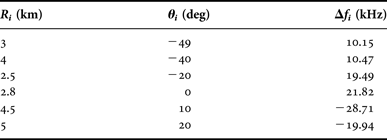
For the simulation purpose, we have considered a 10 GHz FDA, consisting of ten elements with λ/2 inter-element spacing and an initial frequency offset of 10 kHz. As can be inferred from Fig. 4, few locations of the interference source are given below. In Table 1, for every location, the frequency offset so obtained from (14) has also been mentioned.
Table 1. Locations of the interference source and the frequency offsets so obtained.

Figure 8(a) shows nulls of the beampattern in angle keeping range fixed, whereas Fig. 8(b) shows null placement in range keeping angle fixed. Sharp nulls of the order of −300 dB in all the cases validate the proposed methodology and also show the versatility of the proposed formulation, which can cast nulls at any combination of (R, θ). Due to the periodic nature of the FDA beampattern, one can notice periodic nulls at different (R, θ) pairs. However, deepest nulls appear only at the specified locations of the interferer as obtained by the proposed methodology. In order to present a clear view of the nulls, position of the interferer with coordinates (3 km −49°) is considered. In Fig. 9(a), clear nulls at locations other than the desired locations can be witnessed, of the order of −40 to −50 dB. Periodicity of the null in LFDA beampattern is c/NΔf, as deduced from (10). For Δf of 10.15 kHz and 10 element array, nulls are repeated every 3 km. This can be verified from Fig. 9. So not only other nulls are appearing but are also periodic. In Fig. 9(b), three-dimensional (3D) absolute field representation also verifies nulls at other range–angle pairs, as shown by the data tips.

Fig. 8. (a) Field versus angle with time and range fixed. (b) Field versus range with time and angle fixed.

Fig. 9. Periodicity of nulls (a) 2D representation, (b) 3D representation.
Figures 10(a)–10(f) show 3D range angle-dependent beampatterns for null placement at all the six selected locations of the interferer. For clarity of the figure, absolute values of the field are plotted which show sharp nulls with extremely low values.

Fig. 10. Range–angle beampattern of FDA with the proposed offset for (a) (−49°, 3 km), (b) (−40°, 4 km), (c) (−20°, 2.5 km), (d) (0°, 2.8 km), (e) (10°, 4.5 km), and (f) (20°, 5 km).
IV. CONCLUSIONS AND FUTURE WORK
This paper has provided an implementable cognitive null steering solution in FDA radars. As shown through simulations, frequency diversity provides extra maneuverability and higher degree of freedom for precise null placement i.e. null placement in angle as well as in range, which is seldom possible with PAR. The MUSIC estimation method provides the exact DOA estimation. The NN used as time series predictor for the next location (range, angle) of interference source behaves adequately with minimum errors and helps keeping a track of the interference source. Precise and deepest nulls are placed at the estimated next positions of the interference source, thus minimizing the returns from interferer, which can potentially enhance system performance in terms of SINR. Simultaneous placement of beam maximum at the target and null at the interference source is one of our future aims. Similarly multiple null steering methods for the suppression of multiple interferers is an avenue still to be explored in FDA radars.
ACKNOWLEDGEMENT
We want to thank our peers and administration for their valuable support.
 Sarah Saeed is a Ph.D. Scholar at Air University and is also acting as an Assistant Professor in Electrical Engineering Department in the same university since 2007. Her main research interests are design and optimization of radar systems.
 Ijaz Mansoor Qureshi is a full Professor in the Department of Electrical Engineering, Air University. He has about 300 publications technical. His main research interests are array signal processing, communication systems, radars systems, and adaptive beamforming.
 Abdul Basit is a Ph.D. Scholar at International Islamic University, Islamabad and is also acting as a Lecturer in Electrical Engineering Department in the same university since 2007. His main research interests are cognitive radar systems.
 Ayesha Salman is a Ph.D. Scholar at Air University, Islamabad and is also acting as a Lecturer in Electrical Engineering Department in the same university since 2006. Her main research interests are cognitive radio networks.
 Waseem Khan is a Ph.D. Scholar at Air University and is also acting as an Assistant Professor in Electrical Engineering Department in the same university since 2009. His main research interests are radar systems and signal processing.