3.1.1 Variable physical properties beyond OB approximation

Figure 1 shows that dynamic viscosity ${\it\mu}$ , conductivity $k$ and also Prandtl number $Pr$ vary with temperature. ${\it\mu}$ and $k$ are computed with (2.4). As shown in figure 1(a), ${\it\mu}$ and $k$ vary greatly with $T$ in the NOB case. For example, ${\it\mu}$ is reduced by more than 50 % near the cold wall and increased by approximately 40 % near the hot wall when ${\it\epsilon}=0.6$ . It is also observed that $k$ varies with $T$ a bit faster than ${\it\mu}$ . In figure 1(b), $Pr$ also varies with temperature because of the asynchronous changes of ${\it\mu}$ and $k$ . The red solid vertical line helps to reveal that for the reference state and OB case $Pr=0.71$ . Compared with the OB approximation, the Prandtl number increases near the cold top wall and decreases near the hot bottom wall. Even with ${\it\epsilon}=0.6$ , the Prandtl number is approximately 0.8 which is still less than unity, and thus the viscous BL is always nested in the thermal one. Since the change of thermal pressure is relatively small (Le Quéré et al. Reference Le Quéré, Weisman, Paillère, Vierendeels, Dick, Becker, Braack and Locke2005) and perfect gas is used as the working fluid, ${\it\rho}=p/T$ becomes larger near the cold wall and smaller near the hot wall. Thus near the cold wall, kinematic viscosity ${\it\nu}={\it\mu}/{\it\rho}$ becomes smaller and similarly for the thermal diffusivity ${\it\kappa}=k/{\it\rho}c_{p}=k/{\it\rho}$ . Near the hot wall, ${\it\nu}$ and ${\it\kappa}$ are increased. As regards the thermal isobaric expansion coefficient, clearly ${\it\alpha}=1/T$ becomes larger in magnitude near the cold wall.

Figure 2. Log–log plots of $Nu$ as a function of $Ra$ for various temperature differentials. (a) OB approximation, (b) ${\it\epsilon}=0.2$ , (c) ${\it\epsilon}=0.4$ , (d) ${\it\epsilon}=0.6$ . Grey square symbols are flow pattern $P_{11}$ . Grey triangular symbols are flow pattern $P_{12}$ . Grey circle symbols are specially mixed patterns with both $P_{11}$ with definite period and $P_{12}$ with random period in the process of flow reversals. Red symbols ‘ $+$ ’ represent where there exist flow reversals and the dashed lines denote that the growth of corner rolls is observed only once and $P_{12}$ is achieved in the end.

3.1.2 New flow reversals

Figure 2 shows plots of $Nu$ as a function of $Ra$ for various temperature differentials and the phenomenon of the co-existence of multiple solutions is identified. In general, two flow patterns $P_{11}$ and $P_{12}$ are identified where $P_{11}$ has one dominant cavity-sizable roll with two diagonally arranged secondary rolls and $P_{12}$ has two vertically stacked dominant rolls. Under the OB approximation, pattern $P_{11}$ is unchanged in the full Rayleigh number range. When the temperature differential increases, with ${\it\epsilon}\geqslant 0.2$ , we observed the corner roll growth at Rayleigh numbers denoted by dashed lines and symbols ‘ $+$ ’, and the symbols ‘ $+$ ’ in particular show cases of flow reversals. Phenomenally, flow reversal is caused by corner roll growth. However, corner roll growth does not always result in flow reversal. Dashed lines mean that the corner roll in pattern $P_{11}$ grows in size but ends up with pattern $P_{12}$ . It is conjectured that sometimes, in the phase space the trajectory of pairs of $P_{11}$ passes by the stable pattern $P_{12}$ and is attracted by the stationary point or limiting cycle of $P_{12}$ . In figure 2(d), it is noteworthy that with strong NOB effects two counter-rotating flow patterns $P_{11}$ could switch back and forth with an unstable intermediate pattern $P_{12}$ in $3\times 10^{6}\leqslant Ra\leqslant 4\times 10^{6}$ . In short, as ${\it\epsilon}\geqslant 0.2$ , we could observe the growth of the cold corner roll at a large range of Rayleigh numbers, for some of which cession-led flow reversals are clearly found. To some extent, the newly found flow reversals may be related to the tendency for symmetry restoration of an asymmetric system.

Currently, the vertical velocity component $w$ at $y=0.1$ and $z=0.5$ is selected as an indicator of flow reversal, since the flow field is well organized by LSC, corner rolls and BLs rather than plumes (Breuer & Hansen Reference Breuer and Hansen2009; Chandra & Verma Reference Chandra and Verma2011). Figure 3(a,b) shows the time evolution of $w$ at $Ra=7\times 10^{5}$ and $10^{7}$ , in which flow reversals can be clearly found. At $Ra=7\times 10^{5}$ , the flow is laminar and the period of reversal is definite. At $Ra=10^{7}$ , the flow is chaotic or turbulent with random periods of reversal. As shown by the inset closeups, at $Ra=7\times 10^{5}$ , the flow reversals only include pattern $P_{11}$ which circulates clockwise, counter-clockwise and back (Sugiyama et al. Reference Sugiyama, Ni, Stevens, Chan, Zhou, Xi, Sun, Grossmann, Xia and Lohse2010; Chandra & Verma Reference Chandra and Verma2013). At $Ra=10^{7}$ , flow pattern $P_{12}$ sometimes appears, which has been recently reported by Podvin & Sergent (Reference Podvin and Sergent2015). In other words, the process of flow reversals in this case contains two flow patterns $P_{11}$ and $P_{12}$ .

Figure 3. Time evolution of vertical velocity component at 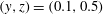$(y,z)=(0.1,0.5)$ . (a) $Ra=7\times 10^{5}$ , ${\it\epsilon}=0.4$ ; (b) $Ra=10^{7}$ , ${\it\epsilon}=0.4$ . Green solid diamonds correspond to the closeups near them. In (a), times for the two closeups are 1560 and 3270. In (b), times for the three closeups are 1250, 6250 and 18 750. Corresponding flow animations are shown in supplementary movies 1 and 2, available at http://dx.doi.org/10.1017/jfm.2016.338.

Figure 4. Snapshots of four characteristic temperature fields during a half-period of a flow reversal. Red indicates hot fluid and blue cold fluid. Black arrows represent velocity vectors. $Ra=10^{7}$ , ${\it\epsilon}=0.4$ and the time is near $t=17\,000$ in figure 3(b).

3.2.1 Kinematics of reversals

In the work of Sugiyama et al. (Reference Sugiyama, Ni, Stevens, Chan, Zhou, Xi, Sun, Grossmann, Xia and Lohse2010), flow reversals occur due to the growth in size of corner rolls. The flow satisfies top-down symmetry under OB approximation, two diagonally arranged corner rolls grow simultaneously and merge as a new LSC, and finally the preceding LSC is then divided into two new corner rolls (see also Chandra & Verma Reference Chandra and Verma2013). When NOB effects are included, the top-down symmetry breaks, which greatly influences the behaviour of large-scale dynamics and consequently flow reversal. Figure 4 shows a half-period of flow reversal for $Ra=10^{7}$ and ${\it\epsilon}=0.4$ . It is found that only the top-right corner roll in figure 4(a), which is larger in size and more energetic than the bottom-left one, grows alone and eventually replaces the LSC. The preceding LSC is divided into two parts. One merges with the existing left hot corner roll and both of them die away finally. The other shrinks to a new hot corner roll near the right wall. Compared with the OB case, two major differences in the reversal process have been identified in the NOB case. On the one hand, the hot corner roll with comparatively small size is weak and no visible expansion is observed. This is caused by both buoyancy reduction and larger viscous dissipation near the bottom wall due to the higher temperature. On the other hand, only the single cold corner roll grows and when it reaches the opposite wall, the buildup of a new cold corner roll can be seen in figure 4(b), which is caused by adverse pressure gradient. As seen in figure 4(c), a portion of descending hot plume is observed near the right wall. Huang & Zhou (Reference Huang and Zhou2013) found that there exists strong counter-gradient local heat flux with a magnitude much larger than the global Nusselt number $Nu$ . Two mechanisms were proposed to be responsible for the local reverse heat flux. One is due to bulk dynamics and the other comes from the competition between LSC and corner rolls. It is the first mechanism that is recognized presently. This descending hot plume forced by the velocity field originated from the newly formed bulk produces counter-gradient local heat flux which results in even negative average $Nu$ (Chandra & Verma Reference Chandra and Verma2013; Yanagisawa, Hamano & Sakuraba Reference Yanagisawa, Hamano and Sakuraba2015; Huang & Xia Reference Huang and Xia2016).

Figure 5. (a) Distribution of dilation defined by equation (2.6); only the field of the top-left quarter of the box is shown. $Ra=10^{7}$ , ${\it\epsilon}=0.4$ . (b) Sketch of th control volume related to (a). The time is the same as figure 4(d). Dashed lines are contours of vorticity density of zero value and roughly serve as dividing lines between LSC and corner rolls.

3.2.2 Physical mechanism from dynamics of vorticity transport

As aforementioned, the growth of the single cold corner roll induces flow reversals when NOB effects are included, but the physical mechanisms corresponding to the corner roll growth have not yet been analysed. In this subsection, we attempt to understand the detailed mechanisms of growth of the cold corner roll from the perspective of vortex dynamics. First, based on the low-Mach-number momentum equations (2.2) and Reynolds transport theorem, we derive the vorticity transport equation in the NOB case. It is believed that vorticity in corner rolls and LSC is in dynamic balance under OB approximation. And thus possibly the balance is broken by vorticity generation in corner rolls when flow reversals occur with NOB effects. Our aim is to pinpoint which terms in this equation are dominant for the vorticity generation in the corner roll. The vorticity transport equation can be expressed as

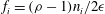
(3.1) $$\begin{eqnarray}\displaystyle \displaystyle \frac{\partial }{\partial t}\int _{V_{0}}\,\text{d}V{\it\Omega}_{i} & = & \displaystyle \underbrace{-\oint _{S_{0}}n_{j}\,\text{d}S{\it\Omega}_{i}u_{j}}_{\text{I}}\underbrace{-\int _{V_{0}}\,\text{d}V{\it\Omega}_{i}\partial _{j}u_{j}}_{\text{II}}\underbrace{-\int _{V_{0}}\,\text{d}V\frac{1}{T}\unicode[STIX]{x1D626}_{ijk}\partial _{j}T\partial _{k}{\rm\pi}}_{\text{III}}\nonumber\\ \displaystyle & & \displaystyle \displaystyle +\,\underbrace{\left(\frac{Pr}{Ra}\right)^{0.5}\int _{V_{0}}\,\text{d}V\frac{1}{T}\unicode[STIX]{x1D626}_{ijk}\partial _{j}(T\partial _{l}{\it\tau}_{lk})}_{\text{IV}}\underbrace{-\frac{1}{2{\it\epsilon}}\int _{V_{0}}\,\text{d}V\frac{1}{T}\unicode[STIX]{x1D626}_{ijk}\partial _{j}Tn_{k}}_{\text{V}},\end{eqnarray}$$

where $S_{0}$ and $V_{0}$ are the control surface and volume in figure 5(b). The control volume in (3.1) is roughly surrounded by the zero-value vorticity lines near the top-left corner and two other straight lines $y\approx 0.35$ and $z\approx 0.75$ . Since 2D RBC is considered, the term ‘control volume’ is actually a fixed area and $S_{0}$ the line surrounding it. With no stretching and tilting of the vortex filament, ${\it\Omega}_{i}={\it\rho}{\it\omega}_{i}$ is the vorticity density with $i=1$ in 2D simulation. $\unicode[STIX]{x1D626}_{ijk}$ is the permutation tensor. The left integral term is the time rate of change of total vorticity surrounded by $S_{0}$ . On the right-hand side of the equality, term I means vorticity transport by convection; term II represents the change of vorticity by dilation or compressibility, vanishing under the OB limit; term III is the interaction of gradient of temperature and hydrodynamic pressure, i.e. baroclinity; term IV is the vorticity diffusion by viscous force; and the last term V indicates the vorticity generation by buoyancy force.

Figure 6. Intensities of contributions to the time rate of change of vorticity in the control volume in ten snapshots. The intensities are normalized by the grey area in figure 5(b) for integration. $Ra=10^{7}$ , ${\it\epsilon}=0.4$ .

Figure 5(a) shows distributions of dilation for $Ra=10^{7}$ with ${\it\epsilon}=0.4$ . LSC and corner rolls could be divided by black-dashed auxiliary vorticity contour lines with zero value. Qualitatively, term I becomes stronger when the Rayleigh number increases and subsequently more plumes detach from the unstable corner roll. For term II, the maximum and minimum regions of dilation in figure 5(a), denoted ‘1’, ‘2’ and ‘3’, are all approximately within the corner roll. The zero contour line of vorticity density goes through ‘1’. The maximum ‘2’ and minimum ‘3’ are near each other, and thus their contributions would approximately offset each other. Since low-Mach-number flow with large temperature difference is barotropic, term III, baroclinity, may possibly change with temperature gradient. The contribution should be specified quantitatively. Term IV, associated with viscosity force, is always negative, corresponding to the vorticity diffusion and dissipation. When the Rayleigh number increases, the viscous effect decreases and concentrates near the wall and the thin region between the corner rolls and LSC. The last term, V, shows the interaction between gravity and temperature gradient. When NOB effects become stronger, it can be affected by $T_{,i}/2{\it\epsilon}$ and the reciprocal of temperature $1/T$ . The coefficient $1/T$ of terms III and V introduces some extent of asymmetry between the diagonally arranged top and bottom corner rolls. The asymmetry in term IV is ${\it\mu}$ in ${\it\tau}_{ij}$ rather than $1/T$ .

To quantify the contributions of the five terms in (3.1) to the time rate of change of vorticity, we compute their normalized intensities in ten snapshots at $Ra=10^{7}$ with ${\it\epsilon}=0.4$ in figure 6. Ten snapshots with an equal time interval are carefully chosen to ensure that they are all at the initial phase of a flow reversal. Compared to the duration of growth of corner rolls, the ten snapshots are taken within a short time. In general, terms IV and V are dominant. From flow fields, term I is found to be related to the oscillations of unstable corner rolls where plume detachment from the corner rolls by convection causes vorticity and energy loss. The plume detachment could also be found in the OB case (Sugiyama et al. Reference Sugiyama, Ni, Stevens, Chan, Zhou, Xi, Sun, Grossmann, Xia and Lohse2010). Plume detachment occurs frequently, which could interrupt the growth of corner rolls whether or not NOB effects are included. In NOB cases, term II is small and negligible, which is consistent with the previous qualitative analysis. Term III is of an order of magnitude of 0.01 and thus can be neglected as well. This is because the temperature gradient within the cold corner rolls may still be small and so is the gradient of velocity, although ${\it\epsilon}$ is increased up to 0.4.

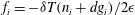
Figure 7. Buoyancy force $f_{i}=\displaystyle ({\it\rho}-1)n_{i}/2{\it\epsilon}$ varying with height $z$ providing linear distribution of temperature 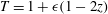$T=1+{\it\epsilon}(1-2z)$ . The black hollow up-triangles represent the distribution of equivalent buoyancy force with respect to the reference state with modelled gravity acceleration. The red solid line is to show the case under OB approximation for comparison.

As stated previously, the interesting difference is that only the cold corner roll grows, while the hot corner roll is found to be nearly quiescent. As we can see in figure 6, terms IV and V are two decisive factors. It is obvious that term V is always positive and thus of vital importance in vorticity generation. The asymmetries caused by $1/T$ (isobaric thermal expansion coefficient ${\it\alpha}=1/T$ ) in this term other than $1/T_{0}=1$ under OB approximation may play key roles in the growth of the cold corner roll. Term V originates from the buoyancy force $f_{i}={\it\delta}{\it\rho}n_{i}/2{\it\epsilon}$ in (2.2). Under the OB approximation, $f_{i}=-{\it\delta}Tn_{i}/2{\it\epsilon}$ is proportional to ${\it\delta}T$ while this relation does not hold in the NOB case $f_{i}=(1/T-1)n_{i}/2{\it\epsilon}\approx (-{\it\delta}T+{\it\delta}^{2}T)n_{i}/2{\it\epsilon}$ with ${\it\delta}T=T-1$ . In figure 7, due to NOB-effects-led asymmetry, the buoyancy force has increased by up to 150 % on the cold wall and reduced by approximately 40 % near the hot wall. Equivalently, we modified the gravity acceleration to model a similar buoyancy force based on the OB approximation. In figure 7, the up-triangular symbols display a buoyancy force to model that of ${\it\epsilon}=0.4$ . The expression of acceleration is $f_{i}=-{\it\delta}T(n_{i}+dg_{i})/2{\it\epsilon}$ with 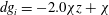$dg_{i}=-2.0{\it\chi}z+{\it\chi}$ in which ${\it\chi}={\it\chi}_{1}=0.3$ when $z\leqslant 0.5$ and ${\it\chi}={\it\chi}_{2}=0.7$ when $z>0.5$ . By adding this equivalent buoyancy force to the OB case, not surprisingly, we reproduced flow reversals (see supplementary movie 3). In this case, the hot corner roll still grows at a smaller rate than its cold counterpart, although the buoyancy force is reduced near the hot wall. The modified buoyancy force by NOB effects increases the probability of the balance breaking (Sreenivasan et al. Reference Sreenivasan, Bershadskii and Niemela2002; Liu et al. Reference Liu, Zhang and others2008) between the corner roll and LSC, and thus leads to flow reversal. In addition, the variation in viscous dissipation in term IV by NOB effects, as seen in figure 1, is also very important for the growth of the cold corner roll. Near the hot wall, viscous dissipation is largely enhanced, which helps to suppress the growth of the hot corner roll. Conversely, the viscous dissipation near the cold wall is considerably attenuated, which promotes the growth of the cold corner roll. Moreover, it is noteworthy that thermal conductivity $k$ is also temperature-dependent. Although thermal conductivity $k$ does not appear explicitly in vorticity transport equation (3.1), as stated by Sugiyama et al. (Reference Sugiyama, Ni, Stevens, Chan, Zhou, Xi, Sun, Grossmann, Xia and Lohse2010), small $k$ near the cold wall has small thermal dissipation similar to ${\it\mu}$ . In figure 1(b), the Prandtl number does not change much and is always smaller than one. Therefore the effect of change of the Prandtl number could probably be ignored.

3.2.3 Mass transport and the role of BLs

In the previous section, we conclude that the asymmetry of isobaric thermal expansion coefficient ${\it\alpha}=1/T$ is the point that results in the growth of the cold corner roll. A very important issue, from the point of view of conservation, is that the process of mass transport between corner rolls and other regimes is still unknown. Figure 8 shows the distribution of density near the top-left corner and the trajectories of two ‘tracer particles’. The trajectories are computed by the predictor–corrector method with accuracy of second order, which is consistent with that of the present code. The corner roll and LSC interact with the top wall and two parts of the BLs form with the joint point marked ‘O’. When the corner roll grows, point ‘O’ moves rightward. Figure 8(a) shows that the density in the cold corner roll changes from $1.6$ to approximately $1$ . The initial positions of the tracer particles are located on either side of the joint point ‘O’. In figure 8(b), tracer particle ‘A’ is initially located in the left part of the BL and we find that it always circles in the corner roll and is superimposed by a small velocity pointing to LSC, corresponding to the expansion of the corner roll. The tracer particle ‘B’ is located initially in the right part of the BL related to LSC. It is found that the tracer particle ‘B’ moves rightward initially (black arrow in figure 8(c)) and circles the bulk. After six rounds, when the time is approximately 390 in figure 8(c), tracer particle ‘B’ turns left into the corner roll at the seventh round. At this moment, the flow field shows us that the joint point ‘O’ has a horizontal location $y\approx 0.5$ so that particle ‘B’ just after the six rounds has been contained in the left part of the BL. The trajectory of tracer particle ‘B’ clearly shows how the fluid parcel transports from LSC into the cold corner roll. This process could partially explain why the cold corner roll grows from the point of view of mass conservation. Then, it is easy to imagine that when the joint point ‘O’ moves to $y=1$ , all the fluid parcels in the BL would transport into the cold corner roll and the preceding bulk could eventually be replaced. Moreover, the asymmetry by NOB effects manifests itself as a thinner BL near the cold upper plate. We could speculate that the relatively small viscosity there helps to transport mass from the BL to the corner roll.

Figure 8. (a) Distribution of density near top-left corner. (b) Trajectory of ‘tracer particle’ A for time duration of 400 dimensionless time units. (c) Trajectory of ‘tracer particle’ B for time duration of 400 dimensionless time units. $Ra=7\times 10^{5}$ , ${\it\epsilon}=0.4$ . Initial coordinates of A and B are $y=0.1978$ , $z=0.9862$ and $y=0.3974$ , $z=0.9862$ , respectively shown as black squares. The initial locations are also shown in (b) and (c) and the nearby black arrows reveal the moving directions at the beginning.