1. Introduction
Chemical reactions with nonlinear kinetics in which substances transform into each other can give rise to a complicated dynamics (Prigogine & Nicolis Reference Prigogine and Nicolis1977). If reagent concentrations change both in time and space, then one should account for molecule diffusion, which causes the substances to spread out over space. The problems of reaction–diffusion are mathematically described in terms of nonlinear evolution equations in partial derivatives and have been extensively studied for more than sixty years (Prigogine & Nicolis Reference Prigogine and Nicolis1977; Grindrod Reference Grindrod1996; Pismen Reference Pismen2006). Reaction–diffusion systems have demonstrated a remarkable set of complex dynamical phenomena. These include periodic, quasiperiodic and chaotic changes in concentration, travelling waves of chemical reactivity and stationary Turing patterns (Epstein & Pojman Reference Epstein and Pojman1998). We should remember, however, that the transport of substances by bulk motion of a fluid is ignored in reaction–diffusion problems that deal exclusively with the diffusive transport.
Although the chemo-hydrodynamic pattern formation in a system of two reacting fluids was experimentally observed as early as 1888 (Quincke Reference Quincke1888), these studies were mainly descriptive by nature due to the complexity of these processes. However, a really consistent detailed study of the reaction–diffusion processes coupled with hydrodynamic phenomena started only a century later, since it was stimulated by many important technological applications including oil refining (Dupeyrat & Nakache Reference Dupeyrat and Nakache1978), photochemical polymerization (Evans & Uri Reference Evans and Uri1949; Belk et al. Reference Belk, Kostarev, Volpert and Yudina2003), combustion processes (Zeldovich & Kompaneets Reference Zeldovich and Kompaneets1960), separation of uranium ore (Thomson, Batey & Watson Reference Thomson, Batey and Watson1984), chemical reactor design and technology (Levich, Brodskii & Pismen Reference Levich, Brodskii and Pismen1967; Jakobsen Reference Jakobsen2008), external control of continuous-flow microreactors (Jensen Reference Jensen2001; Bratsun et al. Reference Bratsun, Kostarev, Mizev, Aland, Mokbel, Schwarzenberger and Eckert2018; Bratsun & Siraev Reference Bratsun and Siraev2020), chemisorption (Lambert Reference Lambert1997; Karlov et al. Reference Karlov, Kazenin, Baranov, Volkov, Polyanin and Vyazmin2007), etc. Starting with the monograph (Levich Reference Levich1962), the interaction between reaction–diffusion phenomena and hydrodynamic instabilities has attracted increasing interest because chemically induced changes of fluid properties, such as concentration, density, viscosity and surface tension, may result in the instabilities, which exhibit a large variety of convective patterns.
A second-order exothermic neutralization reaction has been actively studied in recent years because of a comparatively simple, albeit nonlinear, kinetics. If two miscible solutions of reagents  $\textrm {A}$ and
  $\textrm {B}$ reacting according to the simple kinetic scheme
  $\textrm {A}+\textrm {B} \to \textrm {C}$ with a high reaction rate, are brought into contact, then a reaction front arises. This situation was thoroughly studied in several works (Gálfi & Rácz Reference Gálfi and Rácz1988; Koza & Taitelbaum Reference Koza and Taitelbaum1996) within a pure reaction–diffusion approach without gravity, and a scaling theory was applied to an infinite system. If the reaction takes place under gravity, this may result in various buoyancy-driven instabilities, which have been intensively studied both experimentally and theoretically in the last decade (Zalts et al. Reference Zalts, El Hasi, Rubio, Urena and D'Onofrio2008; Almarcha et al. Reference Almarcha, Trevelyan, Riolfo, Zalts, El Hasi, D'Onofrio and De Wit2010; Hejazi & Azaiez Reference Hejazi and Azaiez2012; Tsuji & Müller Reference Tsuji and Müller2012; Carballido-Landeira et al. Reference Carballido-Landeira, Trevelyan, Almarcha and De Wit2013; Kim Reference Kim2014, Reference Kim2019; De Wit Reference De Wit2020). When a denser solution is placed above a less dense one, a Rayleigh–Taylor (hereinafter abbreviated to RT) instability occurs, deforming the initial contact surface into finger-shaped convective currents (Fernandez et al. Reference Fernandez, Kurowski, Petitjeans and Meiburg2002; Trevelyan, Almarcha & De Wit Reference Trevelyan, Almarcha and De Wit2011; Carballido-Landeira et al. Reference Carballido-Landeira, Trevelyan, Almarcha and De Wit2013). In the reverse case, when a less dense solution is placed above a denser one, the instabilities may occur due to differential-diffusion effects, resulting in the development of either a double-diffusive (DD) instability or a diffusive-layer-convection (DLC) instability. However, in contrast to the non-reactive case, where these instabilities develop symmetrically with respect to the initial contact line (Fernandez et al. Reference Fernandez, Kurowski, Petitjeans and Meiburg2002), the neutralization reaction breaks the symmetry, and the convective motion is induced solely on one side of the reaction front (Almarcha et al. Reference Almarcha, Trevelyan, Riolfo, Zalts, El Hasi, D'Onofrio and De Wit2010; Lemaigre et al. Reference Lemaigre, Budroni, Riolfo, Grosfils and De Wit2013). This happens because different diffusion effects arise between the reactant
  $\textrm {A}$ (or
  $\textrm {B}$) and the reaction product
  $\textrm {C}$ in each layer rather than between the reactants since they cannot diffuse through the reaction zone due to a high reaction rate. All these studies show that the neutralization reaction which takes place in miscible solutions does not give rise to a new type of instability, but it significantly changes the development of the well-known instability mechanisms. In Trevelyan, Almarcha & De Wit (Reference Trevelyan, Almarcha and De Wit2015), the authors attempted to classify all possible types of the buoyancy-driven instabilities occurring in two-layer miscible systems by analysing the large time asymptotic density profiles. This classification, however, is not complete because very soon new types of instabilities were experimentally discovered (Bratsun et al. Reference Bratsun, Kostarev, Mizev and Mosheva2015, Reference Bratsun, Mizev, Mosheva and Kostarev2017).
The most important finding is the experimentally detected shock-wave-like structure (hereinafter SW), which could be excited assuming that the densities of the upper and lower layers are close in value (Bratsun et al. Reference Bratsun, Mizev, Mosheva and Kostarev2017). This mass transfer mode was fundamentally different from the common fingering process since a wave with a perfectly planar front and a nearly discontinuous change in density across the wavefront occurs. The most surprising thing was that the reaction in a typical laboratory cuvette ended in a matter of minutes due to the complete burnout of the reagents (instead of tens of hours in the DD or DLC modes of convection). Some general explanations of this effect are given in Bratsun (Reference Bratsun2017); Bratsun et al. (Reference Bratsun, Mizev, Mosheva and Kostarev2017).
Another type of a new pattern formation was reported in Bratsun et al. (Reference Bratsun, Kostarev, Mizev and Mosheva2015). It was shown that it occurs due to concentration-dependent diffusion (hereinafter, CDD). In general, such a concentration dependence exists in most systems (Crank Reference Crank1975), but often, e.g. in dilute solutions, it is weak and the diffusion coefficient can be assumed constant. There are only a few examples illustrating the CDD effect in fluid mechanics. They include quite exotic problems of membrane transport (Ash & Espenhahn Reference Ash and Espenhahn2000) and colloid ultrafiltration (Bowen & Williams Reference Bowen and Williams2001), where the basic fluid flow is just slightly modified. However, the potential of this phenomenon was revealed, particularly in the problems dealing with chemical reactions. As it turned out, the CDD effect could lead to an overall transformation of the density profile during the system evolution. In Bratsun et al. (Reference Bratsun, Stepkina, Kostarev, Mizev and Mosheva2016), we have shown that the CDD convection results in the development of a perfectly periodic convective structure oriented parallel to the reaction front and perpendicular to the gravity force. This type of pattern formation is also qualitatively different from the typical fingering process during either a DD or a DLC.
Thus, these new modes of chemoconvection do not fit into the classification given in the paper (Trevelyan et al. Reference Trevelyan, Almarcha and De Wit2015) and require systematization. Using the short communication format (Bratsun et al. Reference Bratsun, Kostarev, Mizev and Mosheva2015, Reference Bratsun, Mizev, Mosheva and Kostarev2017) made it impossible to describe the obtained results in a consistent manner, especially the results concerning the nonlinear dynamics and system evolution in time. The goal of this work is to provide a comprehensive experimental and theoretical study of the features observed during the evolution of recently obtained pattern formations and to find their place in the general classification of instabilities.
In Part 1 we present the experimental part of the study. The paper is structured as follows. In § 2 we present the system under study in general and introduce a new non-dimensional parameter, which helps to classify the experimental results presented in the next sections. Section 3 contains a detailed description of the design of the experimental set-up and the experimental techniques used. Experimental results are presented in § 4, which is divided into five subsections, each of which deals with the description of different reaction-induced buoyancy instabilities. Finally, in § 5, we summarize the results and make conclusions. In Part 2 (Bratsun, Mizev & Mosheva Reference Bratsun, Mizev and Mosheva2021) we will present the theoretical analysis of the experimental findings and suggest an extended classification of the reaction-induced buoyancy instabilities, which combines the attainments of previous and present studies.
2. Similarity criterion for reaction-induced buoyancy
In this paper we study a two-layer system (figure 1) consisting of miscible solutions of two reactants initially separated by a horizontal contact plane. The upper layer of the system is always of lower density than the lower one, which allows us to exclude the development of a global RT instability from the very beginning of the study. We consider the neutralization reaction taking place between a strong acid and a strong base, initially dissolved in the water layers. From a chemical kinetics viewpoint, neutralization is the reaction of hydronium and hydroxide ions
 \begin{equation} \textrm{H}_3\textrm{O}^{+} + \textrm{OH}^- \to 2\textrm{H}_2\textrm{O}, \end{equation}
which are formed in the course of acid and base dissociation
 \begin{gather} \textrm{HA} + \textrm{H}_{2}\textrm{O} \to \textrm{A}^{-} + \textrm{H}_{3}\textrm{O}^{+}, \end{gather}
 \begin{gather}\textrm{MeOH} \to \textrm{Me}^{+} + \textrm{OH}^-. \end{gather}
The ions of acid residue  $\textrm {A}^{-}$ and alkali metal
  $\textrm {Me}^+$ do not participate in the reaction. Upon completion of the reaction, they form the aqueous solution of a reaction product, namely salt
  $\textrm {MeA}$.

Figure 1. Geometrical configuration of the two-layer miscible system and coordinate axes.
The formation of water molecules during the reaction is accompanied by significant heat realize Q. The standard enthalpy of the reaction is –57  $\textrm {kJ}\cdot \textrm {mol}^{-1}$. The reaction equation in a simplified form is written as
 \begin{equation} \textrm{A} + \textrm{B} \to \textrm{C} + \textrm{Q} ,\end{equation}
where  $A$,
$A$,  $B$ and
  $C$ indicate the concentrations of acid, base and their salt, respectively.
Right after the layers are brought into contact, the reagents diffuse into adjacent layers and react. Since neutralization is one of the fastest reactions (the reaction rate constant is equal to  $k=1.4\cdot {{10}^{11}}\ \textrm {l}\cdot \textrm {mol}^{-1}\cdot \textrm {s}^{-1}$), the reagents cannot penetrate deep and the reaction proceeds in a frontal manner, i.e. within a very narrow reaction zone.
Let us consider the non-dimensional parameter, first introduced by us in Bratsun et al. (Reference Bratsun, Mizev, Mosheva and Kostarev2017), which we further refer as the reaction-induced buoyancy number. It is defined as the ratio of the density of the reaction zone forming  ${\rho }_{rz}$ and that of the solution located in the upper layer
  ${\rho }_{up}$
 \begin{equation} {K}_{\rho}\equiv \frac{{{\rho }_{rz}}}{{{\rho }_{up}}}= \frac{1+{{\beta }_{s}}{{C}_{s}} +{{\beta }_{res}}{{C}_{res}}}{1+{{\beta }_{up}}{{C}_{up}}}.\end{equation}
Here,  $\beta$ is the solutal expansion coefficient,
  $C$ is the molar concentration and the subscripts ‘
 $s$’ and ‘
 $up$’ denote the quantities relating to salt and the reagent dissolved in the upper layer. The last term in the numerator of the (2.5) describes the contribution of the unreacted reagent to the density of the reaction zone. Since during the reaction, each molecule of one of the reagents reacts with one molecule of another reagent, in the case of non-equimolar solutions, i.e. when initial concentration of acid
  ${{A}_{0}}$ and that of base
  ${{B}_{0}}$ are not equal, a part of the molecules of that reagent whose concentration is initially greater remains unreacted in the reaction zone. The parameters
  ${{\beta }_{res}}$ and
  ${{C}_{res}}$ denote the solutal expansion coefficient and concentration of this residual reagent, respectively. For example, in the case
  ${{A}_{0}}<{{B}_{0}}$, the base will be the residual reagent. The concentration of salt and residue can be derived from the following simple relations:
 \begin{equation} {{C}_{s}} =\frac{{{C}_{min }}}{{{\delta }_{D}}},\quad {{C}_{res}} =\frac{{{C}_{max }}-{{C}_{min }}}{{{\delta }_{D}}},\end{equation}
where  ${{C}_{max }}$ and
  ${{C}_{min }}$ denote the maximal and minimal initial concentrations in the pair of reagents. If, e.g. initially
  ${{A}_{0}}<{{B}_{0}}\ {\rm then}\ {C}_{min}=A_0$ and
  ${{C}_{max }}=B_0$ and vice versa. The parameter
  ${{\delta }_{D}}=1+{{{D}_{{slow}}}}/{{{D}_{{fast}}}}$, where
  ${{D}_{slow}}$ and
  ${{D}_{fast}}$ are the diffusion coefficients of the slowest and fastest solutes in the pair of reagents, respectively.
Finally, the parameter (2.5) determines a relative buoyancy force of the narrow reaction zone, which occurs as the reaction proceeds. As an alternative to (2.5), we could introduce an analogue of the Atwood number. However, the reaction-induced buoyancy number for a particular system is calculated quite non-trivially. Therefore, a simple ratio of two densities, in this case, looks preferable to a more complex structure of the Atwood number.
In what follows, we demonstrate that this non-dimensional parameter is a key one of the problems under consideration because, depending on its value, one of the two possible global scenarios develops in the system just after the layers come into contact. If  ${K}_{\rho }\le 1$, then the density of the forming reaction zone turns out to be lower than that of the upper layer, which triggers the development of the local RT instability in the entire upper layer from the very beginning of the process. New portions of the upper reagent, being brought by the convective motion, react and the situation repeats. Thus the flow provides a continuous supply of the reagents and removal of the salt, which in turn enhances the flow itself due to the increase in the conversion rate of the reagents. As a result, the intensive self-sustaining convective motion develops in the whole upper layer. Given the obvious prevalence of convective heat and mass transfer within this scenario, we call this process a convection-controlled mode (hereafter CC).
For  ${K}_{\rho }>1$, the density of the forming reaction zone is higher than that of the upper layer. Therefore, a steady density stratification is settled in the entire two-layer system from the very beginning of the process, which makes it impossible for a convective motion to develop. As a result, a supply of the reagents towards the reaction zone and removal of the salt from it are provided only by diffusion at the initial stage. Later on, as will be shown in the next sections, a hydrodynamic instability may develop at some distance from the reaction front due to differential-diffusion effects. However, the intensity of the convective motion caused by these instabilities is so weak that the characteristic time of the reaction almost coincides with that of diffusion processes estimated on the layer's size scale. Because of the obvious prevalence of diffusive heat and mass transfer within this scenario, we call this process a diffusion-controlled mode (hereafter DC).
It is worth adding here a few words about the physical reasons due to which the CC mode appears. As indicated at the beginning of this section, the essence of the neutralization reaction is reduced to the formation of water in the process of combining hydronium and hydroxide ions. At the same time, the ions of the acid residue and the alkali metal do not participate in the reaction. The volume occupied by the water molecule is larger than the sum of the volume of hydronium and hydroxide ions. This is clearly evident from the fact that  ${{\beta }_{s}}<{{\beta }_{a}}+{{\beta }_{b}}$ for all acid–base pairs and not only for those used in our study. Thus, the neutralization reaction results in a local decrease of the solution density in the reaction zone. This fact makes possible the appearance of the CC regime. On the other hand, the density of the reaction zone, as can be seen from (2.5), is also determined by the contribution of the reagent that remained unreacted in the case of non-equimolar solutions. This further increases the density of the reaction zone in the case of unequal concentrations of reagents. However, this contribution is small, since it is proportional to the difference in the initial concentrations of the reactants, which makes it impossible for a situation where the density of the reaction zone would be greater than the density of the lower solution to occur. Looking ahead, our experiments confirm this fact. We have never observed the appearance of a RT instability in the lower layer similar to that observed in the upper layer at
  ${K}_{\rho }\le 1$.
The sections below provide evidence that the reaction-induced buoyancy number (2.5) allows us to make a priori prediction of the scenario that would happen in the system under given initial conditions.
3. Experimental set-up and measuring techniques
The experiments were carried out in a vertical Hele-Shaw (HS) cell (see figure 1) formed by two plane-parallel glass plates separated by a thin glass spacer of  $h=1.2\ \textrm {mm}$ thickness, which specifies the inner size of the rectangular cavity: width
  $L=2.5\ \textrm {cm}$ and height
  $2H=9.0\ \textrm {cm}$. A two-layer system, composed of the aqueous solutions of the reagents, was formed in the cell before each experiment. One layer represented an aqueous solution of nitric or hydrochloric acid and another an aqueous solution of lithium, sodium, potassium or caesium hydroxide. The initial concentration of the solutions ranged from 0.1 to 3.0 mol l
 $^{-1}$. The characteristics of the solutions are presented in table 1. Depending on the reagent concentration ratio, the upper layer represented either acid or base solutions. The density ratio of the upper and lower layers was always selected in such a way as to form stable density stratification, thereby excluding the development of the RT instability. During the filling of the cell with the upper solution, the lower layer was separated to prevent the premature beginning of the reaction. For this purpose a thin plastic slider was tightly inserted in two narrow (approximately
  $0.3\ \textrm {mm}$) slots made in the middle section of the glass walls. The slider was gently taken out from the cell at the beginning of the experiment. All experiments were performed at room temperature
  $( 24\pm 1 )\,^{\circ }$C.
Table 1. The properties of the aqueous solutions of different solutes used, including the solutal expansion coefficient  $\beta$, the ratio of solutal expansion coefficients of acid and salt
  $\beta _a/\beta _s$, the ratio of solutal expansion coefficients of base and salt
  $\beta _b/\beta _s$, the concentration dependence of the diffusion coefficient
  $D(C)=D_0+k_DC$ and the range of
  $\delta _D$ values in the concentration range used in the experimental study. Note that an acid is a fast diffusing agent and a base is a slow one for all reagent pairs.

Data for solutal expansion coefficients taken from  $^{(a)}$Nikolsky (Reference Nikolsky1965). Data for diffusion coefficients taken from
  $^{(b)}$Nisancioglu & Newman (Reference Nisancioglu and Newman1973),
  $^{(d)}$Wishaw & Stokes (Reference Wishaw and Stokes1954),
  $^{(e)}$Fary (Reference Fary1966),
  $^{(\,f)}$Krienke, Ahn-Ercan & Maurer (Reference Krienke, Ahn-Ercan and Maurer2013),
  $^{(g)}$Bhatia, Gubbins & Walker (Reference Bhatia, Gubbins and Walker1968),
  $^{(h)}$Zaitsev & Avseev (Reference Zaitsev and Avseev1988),
  $^{(i)}$Stokes (Reference Stokes1950) and
  $^{(c)}$our measurements.
Several experimental techniques were performed simultaneously to provide a comprehensive study of physico-chemical processes that accompany the reaction in a liquid medium. The Fizeau interferometer mounted using an autocollimation scheme (see figure 2) was used to visualize the refractive index distribution. In the system under consideration, the refractive index non-uniformity is caused by variations of both solutes’ concentration and the medias' temperature due to reaction exothermicity. Note that the contribution of these mechanisms to the formation of the interference pattern is essentially different, since the temperature coefficient of the refractive index is two orders of magnitude smaller than the concentration one. Taking into account that maximal temperature deviations measured in the experiments (see table 2) did not exceed a few degrees, we can conclude that the interferogram patterns reflect mainly the spatial distribution of species’ concentration. It is worth noting here that only qualitative information can be obtained from the interference patterns because there is no way to restore the concentration distribution of three substances, two reagents and the reaction product, using one-wave interferometry. On the other hand, the study of the temporal evolution of the interference patterns allows us, in some cases, to visualize the convective motion and to gain quantitative information about the flow velocity. Indeed, since the mass diffusive time is three orders of magnitude greater than the viscous time (Schmidt number  $Sc\sim O( {{10}^{3}})$), the concentration isolines turn out to be trapped by the moving liquid, and the interference fringes move together with the liquid medium, thus visualizing the motion pattern. It is important to note here that the use of interference fringes, moving with a liquid medium, as a kind of flow ‘tracer’ is possible only in the case of non-stationary flow. In our study we applied this method only at the very early stage of convective motion formation to measure an average velocity of the plumes being born near the reaction zone.
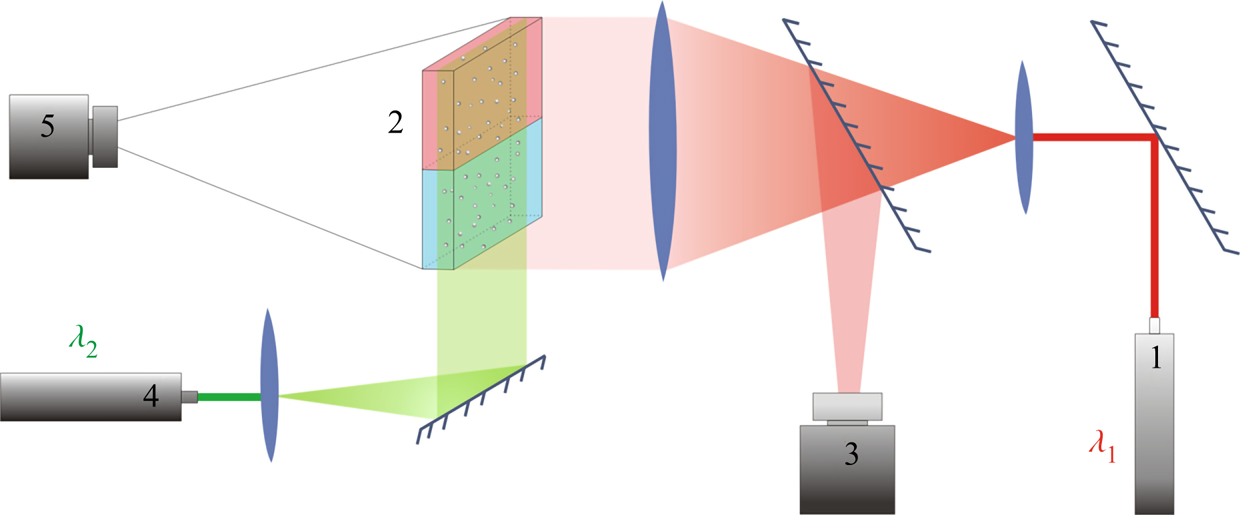
Figure 2. Optical scheme of the experimental set-up for visualization of refraction index distribution and flow velocity field reconstruction. The numbers in the scheme indicate: 1 – the laser with  $\lambda _1 =632.8$ nm used in interferometry, 2 – HS cell, 3 – video camera for recording interferograms, 4 – the laser with
  $\lambda _2 =532$ nm used to create a light sheet, 5 – video camera for recording the light-scattering particle motion.
Table 2. The main characteristics of the processes in the CC and DC regimes.

The silver-coated hollow glass spheres of neutral buoyancy and average diameter of  $20\ \mathrm {\mu }$m were added to the reagent solutions as light-scattering tracers to visualize the convective patterns. The light sheet was oriented in the middle vertical plane of the cavity. The motion of the tracers was recorded by video camera 5 (figure 2). The video records were processed by DigiFlow software to get velocity field characteristics. The use of lasers with different emission wavelengths for interferometry (
 $\lambda _1 =632.8$ nm) and velocimetry (
 $\lambda _2 =532$ nm) purposes, as well as colour filters in the video camera objectives, allowed us to simultaneously observe the refractive index distribution and flow pattern.
A small amount of an acid–base indicator was added to each layer prior to the experiment to visualize the spatial distribution of each reagent and the reaction product. We used a universal indicator which is a mixture of multiple indicators that gradually change colour over a wide pH value range. In some recent studies (Nishimura et al. Reference Nishimura, Tanoue, Watanabe, Itoh and Kunitsugu2006; Almarcha et al. Reference Almarcha, Trevelyan, Riolfo, Zalts, El Hasi, D'Onofrio and De Wit2010; Kuster et al. Reference Kuster, Riolfo, Zalts, El Hasi, Almarcha, Trevelyan, De Wit and D'Onofrio2011), it was reported that the convective patterns and instabilities may be strongly affected by the presence of a colour indicator. To check the possible influence of the indicator on the reaction system, we performed an additional investigation, the results of which have been previously reported in detail (Mosheva & Shmyrov Reference Mosheva and Shmyrov2017). It was found that a universal indicator with relative volume concentration not exceeding  $0.2\,\%$ does not influence the instability scenario and pattern formation process.
A T-type thermocouple was used to control the temperature changes taking place near the reaction front caused by the reaction exothermicity. The thermocouple was fixed on the mechanical actuator which ensured its vertical translation with accuracy  $0.01$ cm.
4. Results and discussion
4.1. Overview of the reaction–diffusion–convection regimes
Analysis of the results of the experiments made with different acid–base pairs in a wide concentration range has revealed the development of reaction–diffusion–convection processes per two different scenarios, depending on the value of the reaction-induced buoyancy number  ${K}_{\rho }$. These scenarios are general for all pairs studied and do not depend on the reagents used. Further, we overview both scenarios in detail and give some quantitative characteristics.
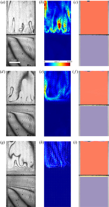
In the case of  ${K}_{\rho }>1$ (figure 3), the stably stratified transition zone begins to form on either side of the reaction front, just after the layers were brought into contact. The concentration changes of both reagents and the reaction product occur within this transition zone, as can be seen from the interferograms presented in figure 3(a,d,g). The liquid inside the zone is immovable and the reagents and the product of reaction are transferred between the layer and the reaction front only by means of the diffusion mechanism. The reaction front moves slowly with characteristic velocity
  $O( {{10}^{-5}} \text {--} {{10}^{-4}} )$ cm s
 $^{-1}$. The zone broadens with time, remaining stably stratified. A weak convective flow with characteristic velocity of the order of
  $O({{10}^{-2}})$ cm s
 $^{-1}$ in the form of fingers always develops in the upper layer above the transition zone (figure 3b,e,h). A weak convective motion may also arise in the lower layer in a certain concentration range. The reasons for the formation of these instabilities and their structure will be considered in greater detail below. Since the convective motion is weak and localized far from the reaction front, being separated by the motionless transition zone, the reaction rate is defined mainly by diffusion processes. Within this scenario, the reaction lasts from a few hours to several days depending on the initial reagent concentration. The reaction rate, defined as the conversion rate of reagents, is on average
  $O( {{10}^{-8}} )$ mol s
 $^{-1}$. The temperature excess due to reaction exothermicity, as measured at the reaction front, is a few tenths of a degree. It is interesting that the characteristic diffusion time, estimated by the vertical size of either layer, is of the order of
  $O( {{10}^{6}} )$ s which almost coincides with the full reaction time within this scenario.

Figure 3. Evolution of two-layer system observed within the framework of the DC regime ( ${K}_{\rho }=1.042$) for the pair of
  $\textrm {HNO}_3$–
 $\textrm {NaOH}$ reactants. From left to right: interference patterns, flow velocity fields, pH distributions. The initial concentrations of the acid and base are equal to 0.3 mol l
 $^{-1}$ and 2 mol l
 $^{-1}$, respectively. The initial contact line between the reactant solutions coincides with the horizontal black line (slot for the slider) in the middle of the cell. Time after the start of the experiment: top row – 110 s; middle row – 1500 s; lower row – 4630 s.
A completely different regime develops in the case of  ${K}_{\rho }\le 1$ (figure 4). Right after the layers are brought into contact, the vigorous plumes are formed above the reaction front. Very soon, the intensive convective motion occupies the whole upper layer, homogenizing it. The characteristic velocity of the liquid motion is of the order of
  $O( {{10}^{-2}} \text {--}{{10}^{-1}} )$ cm s
 $^{-1}$, which is much faster than it is observed in the DC regime. At the same time, the lower layer remains always motionless and homogeneous. The reaction front moves downward with relatively high velocity, of the order of
  $O( {{10}^{-2}} )$ cm s
 $^{-1}$. When the reaction front reaches the bottom of the cuvette, the reaction stops. The reaction lasts from 7 to 15 min, depending on the initial concentration of the reagents. The reaction rate is, on average,
  $O( {{10}^{-5}} )$ mol s
 $^{-1}$. Due to the high conversion rate of the reagents, the temperature excess at the reaction front is a few degrees. Some important characteristics of the described CC and DC regimes are summarized in table 2 for comparison.

Figure 4. Evolution of the two-layer system observed within the framework of the CC regime ( ${K}_{\rho }=0.997$) for the pair of
  $\textrm {HNO}_3$–
 $\textrm {NaOH}$ reactants. From left to right: interference patterns, flow velocity fields, pH distributions. The initial concentrations of the acid and base are equal to 1.5 mol l
 $^{-1}$ and 1.4 mol l
 $^{-1}$, respectively. The initial contact line between reactant solutions coincides with the horizontal black line (slot for the slider) in the middle of the cell. Time after the start of the experiment: top row – 3 s; middle row – 150 s; lower row – 700 s.
4.2. Stability maps
The reaction-induced buoyancy number  $K_\rho$ can be precalculated for each concentration ratio and each pair of reagents to predict the development of one or other regime prior to the experiment. An example of such calculation for the pair
  $\textrm {HNO}_3$–
 $\textrm {NaOH}$ is presented in figure 5(a). The dimensionless quantities
  ${{\beta }_{a}}{{A}_{0}}$ and
  ${{\beta }_{b}}{{B}_{0}}$, being plotted along the
  $x$-axis and
  $y$-axis, are the relative density increments of the acid and base solutions, respectively. The curve, obtaining as a result of intersection of the three-dimensional surface
  ${{K}_{\rho }}=f( {{\beta }_{a}}{{A}_{0}},{{\beta }_{b}}{{B}_{0}} )$ with the plane
  ${{K}_{\rho }}=1$, gives us the boundary between the areas of parameters, in which the CC or DC regime takes place.

Figure 5. Three-dimensional surface characterizing the dependence of  $K_\rho$ on the dimensionless quantities
  $\beta _a A_0$ and
  $\beta _b B_0$ (a) and the map of the regimes (b) calculated for the pair of
  $\textrm {HNO}_3$–
 $\textrm {NaOH}$ reactants. The black solid line is the isopycnic line. The shaded region, adjoining the isopycnic line, is the area of parameters where the CC regime develops. The region, marked with white colour, corresponds to the DC regime. The open and filled symbols indicate the parameters at which the CC and DC modes have been observed in the experiments with the
  $\textrm {HNO}_3$–
 $\textrm {NaOH}$ system, respectively.
The map of regimes obtained in such a way for the  $\textrm {HNO}_3$–
 $\textrm {NaOH}$ pair is shown in figure 5(b). The bisectrix on the map represents the isopycnic line, i.e. the line along which the initial densities of the upper and lower reagent solutions are equal. The equation of the isopycnic line is
  ${{\beta }_{a}}{{A}_{0}}={{\beta }_{b}}{{B}_{0}}$. Here, we neglect a weak nonlinearity of the dependence being of the opinion that, for all substances, the solutal expansion coefficient is constant in the concentration range used. This assumption looks justified, since the maximal error in the definition of the solution density connected with this simplification is within 0.2 %. In the region which lies above the isopycnic line, the upper layer is formed by the acid solution and the lower layer by the base solution. In the lower half of the map, the configuration of the two-layer system is the opposite. The closed area of parameters (shaded area in figure 5(b)), adjacent to the isopycnic line, is the area where
  $K_\rho <1$ and, therefore, the CC mode develops. For all other parameter values,
  $K_\rho >1$ and the DC mode is realized. The symbols in the map indicate the parameters at which the CC mode (open circles) or the DC mode (filled circles) have been observed in the experiments. It is seen that these results are in perfect agreement with the calculations based on (2.5).
The experimental results presented above, as well as their excellent agreement with the results of calculations, confirm the correctness of the physical interpretation of the observed phenomena and the choice of dimensionless governing parameter. Moreover, plotting the regime maps at the stage of planning experiments allows us to predict the regions of existence of different regimes in the problem parameter space, thereby significantly reducing the search stage of the study. In the next sections, we consider each regime in more detail.
It is worth noting here that the maps of regimes, calculated on the base of initial reagent concentrations  $A_0$ and
  $B_0$, give us the possibility to predict one of the two global scenarios realized from the very beginning of the system's evolution. Later on, reduction of the reagent concentrations in the course of reaction leads to shifting of the point describing the position of the system in the regime map. If initial parameters are chosen very near the boundary between the zones, the change of the parameters can result even in a change of regime during later evolution of the system. An example of such transition between global scenarios will be considered in detail in § 4.5. If the initial position of the system in the map is located far from the boundary between the zones the reaction–diffusion–convection processes occur within the initial scenario.
4.3. CC mode
Figure 6 presents the maps of regimes for all reagent pairs. One can see that each map is individual and the position of the curve  ${{K}_{\rho }}=1$, bounding the parameter area within which the CC regime exists changes under varying both an acid and a base in a pair of reagents. Each map was checked in experiments and the results demonstrated a perfect agreement with the calculation.

Figure 6. Maps of regimes for  $\textrm {HCl}$–
 $\textrm {MeOH}$ (a) and
  $\textrm {HNO}_3$–
 $\textrm {MeOH}$ (b) systems. The zone of CC regime existence is denoted with the coloured areas. The region, marked with white colour corresponds to the DC regime.
It is worth noting here that, not only the form of the area where the CC regime exists changes under replacement of one of the reagents, but its depth as well. The three-dimensional surface, shown in figure 5(a), has a pocket-like form with a minimum, always located on the isopycnic line. The depth of the pocket, i.e. the minimal value of  ${{K}_{\rho }}$, depends on the reagents used. The curves, obtained as a result of the intersection of the
  ${{K}_{\rho }}=f( {{\beta }_{a}}{{A}_{0}},{{\beta }_{b}}{{B}_{0}} )$ surface by the vertical plane, containing the isopycnic line, are shown in figure 7. Since the values of
  ${{\beta }_{a}}{{A}_{0}}$ and
  ${{\beta }_{b}}{{B}_{0}}$ are the same along the isopycnic line, any of these quantities can be plotted along the
  $x$-axis. It is seen that the dependencies are non-monotonic, demonstrating the presence of a minimum. The minimal value of
  ${{K}_{\rho }}$ which can be achieved within the region and the location of the minimum significantly depend on the reagent pair.

Figure 7. The dependence of the parameter  $K_\rho$ on the relative density increment of the solution
  ${{\beta }_{b}}{{B}_{0}}$ calculated along the isopycnic line for different pairs of reactants.
Analysing figures 6 and 7 indicates that the size and shape of the parameter area, where the CC regime exists, change significantly when replacing both the acid and the base. Equation (2.5) shows that the value of the parameter  ${{K}_{\rho }}$ depends on the ratio of the diffusion coefficients of the reagents. An increase in
  ${{\delta }_{D}}$ reduces the concentration of salt and residual reagent in the reaction zone after the reaction, which, in turn, results in reduction of
  ${{K}_{\rho }}$ and, consequently, in widening of the zone. Other important parameters are the ratios of the expansion coefficients of each of the reagents to that of salt
  ${{{\beta }_{a}}}/{{{\beta }_{s}}}$ and
  ${{{\beta }_{b}}}/{{{\beta }_{s}}}$. Indeed, an increase in the contribution of the salt into the reaction zone density as compared to that of either of the reagents leads to a faster growth of the reaction zone density and, consequently, a reduction in the zone of the CC regime.
The map of regimes and the dependence  ${{K}_{\rho }}( {{\beta }_{b}}{{B}_{0}})$ were calculated to elucidate the contribution of each of the above quantities. The results of these calculations are presented in table 3. Each row of the table contains the results obtained at two different values of one of the above parameters that differ by 10 %, while the other parameters remained unchanged. It is seen that a decrease in each of the parameters results in a reduction of the zone of the CC mode existence. Moreover, the most significant effect is observed when the ratio of the diffusion coefficients of the reagents changes.
Table 3. Influence of the parameters  $\beta _{b}/\beta _s$,
  $\beta _{a}/\beta _s$ and
  $\delta _D$ on the size and the depth of the zone of CC regime existence.

These findings allow us to better understand the reasons the maps of regimes change on the variation of alkali ions in the pairs of reagents. Analysing the data for  $\textrm {MeOH}\text {--}\textrm {HNO}_{3}$ pairs presented in table 1 shows that the growth of
  ${{{\beta }_{b}}}/{{{\beta }_{s}}}$ is compensated by a reduction of
  ${{{\beta }_{a}}}/{{{\beta }_{s}}}$ when switching from lithium hydroxide to potassium hydroxide. In this situation, the increase in the zone of CC regime existence (see figure 6) and its depth (see figure 7) are mainly due to an increase in
  ${{\delta }_{D}}$. Changing the base to caesium hydroxide leads to a significant decrease in
  ${{{\beta }_{a}}}/{{{\beta }_{s}}}$, which cannot be compensated by a slight increase in
  ${{{\beta }_{a}}}/{{{\beta }_{s}}}$ and
  ${{\delta }_{D}}$. As a result, a significant reduction of the size and depth of the zone of CC regime existence is observed for the
  $\text {CsOH--HNO}_{3}$ pair (see figures 6 and 7).
Another important feature of the regime maps is their asymmetry with respect to the isopycnic line. Analysing the data presented in table 1 shows that the zone of CC regime existence is always wider from the side where the ratio of the solutal expansion coefficient of the upper reagent to that of the salt is smaller. Indeed, the smaller this ratio, the slower the parameter  ${{K}_{\rho }}$ grows as the concentration of the upper reagent increases. For all reagent pairs, except
  $\textrm {LiOH}\text {--}\textrm {HNO}_{3}, ({{{\beta }_{a}}}/{{{\beta }_{s}}})<({{{\beta }_{b}}}/{{{\beta }_{s}}})$, which leads to a wider zone in the upper half of the map, where the upper reagent is acid. The case of
  $\textrm {LiOH}\text {--}\textrm {HNO}_{3}$ is the only reagent pair where
  $({{{\beta }_{a}}}/{{{\beta }_{s}}})>({{{\beta }_{b}}}/{{{\beta }_{s}}})$ and the zone is wider in the lower half of the map. As a quantitative criterion responsible for the degree of asymmetry, one can choose the ratio of the zone width above
  ${{\varDelta }_{1}}$ and below
  ${{\varDelta }_{2}}$, the isopycnic line at a fixed value of
  ${{\beta }_{a}}{{A}_{0}}$ (see the explanations in figure 5(b)). Expressing the concentration values at the zone boundary from the condition
  ${{K}_{\rho }}=1$, we get
 \begin{equation} \frac{{{\varDelta}_{1}}}{{{\varDelta }_{2}}}=\frac{{{\beta }_{b}}( {{\delta }_{D1}}-1 )+{{\beta }_{a}}-{{\beta }_{s}}}{{{\beta }_{b}}( {{\delta }_{D2}}-1 )+{{\beta }_{a}}-{{\beta }_{s}}}\cdot \frac{{{\delta }_{D2}}{{\beta }_{b}}}{{{\beta }_{s}}-{{\beta }_{a}}}. \end{equation}
 This expression is valid for those pairs of reagents for which  ${{\beta }_{a}}<{{\beta }_{b}}$, i.e. the equimolar line lies above the isopycnic line. In the opposite case, when
  ${{\beta }_{a}}>{{\beta }_{b}}$, which is typical only for the pair
  $\textrm {LiOH}\text {--}\textrm {HNO}_{3}$
 \begin{equation} \frac{{{\varDelta }_{1}}}{{{\varDelta }_{2}}}=\frac{{{\beta }_{a}}( {{\delta }_{D1}}-1 )+{{\beta }_{b}}-{{\beta }_{s}}}{{{\beta }_{a}}( {{\delta }_{D2}}-1 )+{{\beta }_{b}}-{{\beta }_{s}}}\cdot ( {{\delta }_{D2}}-1 ). \end{equation}
Here,  ${{\delta }_{D1}}$ and
  ${{\delta }_{D2}}$ are the values of this parameter at the zone boundary located above and below the isopycnic line, respectively. Neglecting the concentration dependence of the diffusion coefficient within the zone, i.e. assuming
  ${{\delta }_{D1}}\approx {{\delta }_{D2}}$, we obtain the following approximate expressions:
 \begin{gather} \frac{{{\varDelta }_{1}}}{{{\varDelta }_{2}}}={{\delta }_{D}}\frac{{{\beta }_{b}}}{{{\beta }_{s}}-{{\beta }_{a}}},\quad \text{if } {{\beta }_{a}}<{{\beta }_{b}}, \end{gather}
 \begin{gather}\frac{{{\varDelta }_{1}}}{{{\varDelta }_{2}}}=( {{\delta }_{D}}-1 ),\quad \text{if } {{\beta }_{a}}>{{\beta }_{b}}, \end{gather}
where  ${{\delta }_{D}}$ is the average value within the zone. The value of this parameter, calculated by formula (4.3) or (4.4), which reflects the degree of asymmetry of the zone of CC mode existence, is presented in table 4 for all the pairs of reagents studied.
Table 4. Values of the parameter that determines the degree of asymmetry of the zone of CC regime existence for all reagent pair used.

The parameter  ${{K}_{\rho }}$ defines not only the development of one or another reaction–diffusion–convection regime but also the convective motion intensity. As a measure of the motion intensity, we used the average velocity in a group of plumes that appear above the reaction zone after the solutions were brought into contact. The velocity was measured at the initial stage when it was constant. Later, the transverse diffusion and interaction between the plumes reduced the plume velocity, and therefore we did not take these results into account. The dependence of the plume velocity, obtained in such a way, on the parameter
  ${{K}_{\rho }}$ is presented in figure 8(a). The results measured for different pairs of the reagents form a unified dependence, the best fit of which is
  $v\sim (K_{\rho }-0.97)^{-4}$. This unification of the experimental data, obtained for different pairs, indicates the universal character of
  ${{K}_{\rho }}$, as a quantity being responsible for the convective motion intensity in the system under study. It is seen that the convective motion rapidly weakens as it approaches the boundary between the CC and DC regimes.

Figure 8. Variation of the plume average velocity measured at the initial stage of an experiment just after the contact of the regents ( $a$) and the reaction front velocity (
 $b$) as a function of
  $K_{\rho }$. The solid lines represent approximating functions that best describe the experimental data.
The convective motion intensity affects the mass transfer rate near the reaction front, which causes the reaction front velocity to change. The variations of the reaction front velocity with change of  ${{K}_{\rho }}$ are presented in figure 8(b). The position of the reaction front was determined from the spatial distributions of the pH value. Note that the value of
  ${{K}_{\rho }}$ uniquely defines the rate of reaction front motion. All experimental points obtained for different reagent pairs and different concentration ranges form a unified dependence, the best fit of which is
  $v_{f}\sim (K_{\rho }-0.98)^{-3}$. It is seen that the reaction front velocity decreases by more than two orders of magnitude when switching from the CC regime to the DC one, which is associated with changes in the mass transfer mechanism, from convective to primarily diffusive.
4.4. DC mode
In this section, we describe some important features of the development of reaction–diffusion–convection processes within the DC regime. Despite of the DC regime's name, mechanical equilibrium is not the only state of the system. Diffusion is only the prevailing mass transfer mechanism near the reaction front, which defines the characteristic time of the reaction–diffusion–convection processes. However, hydrodynamic instabilities can develop at a certain distance from the reaction front due to differential-diffusion effects.
Let us consider these processes in more detail. The fragment of the two-layer system near the reaction front is schematically shown in figure 9. At the reaction front, the reagents are consumed and the reaction product is formed at certain rates. Since the density distribution across the layers is stable at the initial stage in the DC regime, both reagents transfer towards the front only by diffusion. The reaction product, arising at the front during the reaction, spreads upward and downward due to diffusion as well. Taking into account the extremely high rate of the neutralization reaction, one can exclude the penetration of any reagent into the adjacent layer. Then we can assume that each layer contains only two components, one of the reagents and the reaction product, which diffuse towards each other. In this case, the reaction does not affect, to a first approximation, the diffusion processes, and the development of differential-diffusion effects can be examined in each layer independently.

Figure 9. Schematic image of the diffusion processes near the reaction front.
The situation, when two solutes diffuse at different rates towards each other in a vertical direction, was considered in numerous works (Stern & Turner Reference Stern and Turner1969; Taylor & Veronis Reference Taylor and Veronis1996; Pringle, Glass & Cooper Reference Pringle, Glass and Cooper2002; Sorkin, Sorkin & Leizerson Reference Sorkin, Sorkin and Leizerson2002; Trevelyan et al. Reference Trevelyan, Almarcha and De Wit2011). When the upper species diffuse faster, a DLC instability develops. In the opposite case, when the lower species diffuse faster, a DD instability develops in the parameter region  ${{\delta }_{b}}>{{( \varphi {{R}_{b}} )}^{{2}/{3}}}$, where
  ${{\delta }_{b}}={{{D}_{l}}}/{{{D}_{u}}}$ is the ratio of the diffusion coefficients of the lower and upper species,
  $\varphi ={{{C}_{l}}}/{{{C}_{u}}}$ is the ratio of the initial concentrations of the lower and upper species and
  ${{R}_{b}}={{{\beta }_{l}}}/{{{\beta }_{u}}}$ is the ratio of the solutal expansion coefficients of the lower and upper species (Trevelyan et al. Reference Trevelyan, Almarcha and De Wit2015). When
  $1\le {{\delta }_{b}}\le {{( \varphi {{R}_{b}} )}^{{2}/{3}}}$, the system remains stable for all time.
Using the above inequalities, the parameter regions where the DD or DLC instability occurs can be calculated in advance. Figure 10 presents the regime maps calculated for the  $\textrm {HNO}_3$–
 $\textrm {MeOH}$ systems, where the areas of parameters for which different differential-diffusion instabilities occur within the DC regime are indicated. The maps in figure 10(a,c,e,g) were plotted for the upper layer and in figure 10(b,d,f,h) for the lower layer. The light-grey and dark-grey areas indicate zones where the DLC or DD instability develops, respectively. The mechanical equilibrium zone is denoted by the white colour.

Figure 10. Parameter areas for different differential-diffusion instabilities in the DC regime, calculated for the  $\textrm {HNO}_3$–
 $\textrm {MeOH}$ systems: (a)
  $\textrm {HNO}_3$–
 $\textrm {NaOH}$, (b)
  $\textrm {HNO}_3$–
 $\textrm {LiOH}$, (c)
  $\textrm {HNO}_3$–
 $\textrm {KOH}$, (d)
  $\textrm {HNO}_3$–
 $\textrm {CsOH}$. Panels (a,c,e,g) are plotted for the upper layer and panels (b,d,f,h) for the lower layer. The light-grey and dark-grey areas indicate the zones where the DLC or DD instability develops, respectively. The mechanical equilibrium zone is denoted by the white colour.
In all cases, except for the  $\textrm {HNO}_3$–
 $\textrm {LiOH}$ pair, which will be discussed separately, the reagent diffuses faster than salt. That is the reason why the DLC instability always develops in the upper layer at any concentration ratio, regardless of whether the acid (upper half in the maps, presented in figure 10(a,c,e,g)) or the base (lower half in the maps, presented in figure 10(a,c,e,g)) is contained in the upper layer. In the lower layer (figure 10b,d,f,h), where the salt diffusing downwards from the reaction front always has a diffusion coefficient lower than that of the reagent, a DD instability may develop (dark-grey areas in figure 10). At the same time, there are wide parameter areas (white areas in figure 10), where the lower layer remains stationary all the times. The maps were thoroughly tested in a series of experiments, the results of which demonstrated good agreement with calculations. The interferograms, illustrating the development of differential-diffusion instabilities in the areas indicated in the map, are presented in figure 10.
A more interesting situation is observed for the  $\textrm {HNO}_3$–
 $\textrm {LiOH}$ pair. As in the above cases, the salt
  $\textrm {LiNO}_3$ diffuses slower than the acid. However, the diffusion coefficient ratio for the salt and base is not so unambiguous. The salt diffuses slower than the base in the concentration range below 1 mol l
 $^{-1}$, and it diffuses faster in the higher concentration range. This causes both DLC and DD instabilities to occur in the layer, where the salt and base diffuse towards each other, depending on a base concentration. Figure 10(
 $b$) presents the regime maps found in the
  $\textrm {HNO}_3$–
 $\textrm {LiOH}$ system. It is seen that, in the configuration when the nitric acid is placed in the upper layer, the DLC instability develops both in the upper (upper half in the left map in figure 10(b)) layer and in the lower (upper half in the right map in figure 10(b)) layer. The interferograms illustrating this situation are inserted in the corresponding halves of the maps. In the reverse configuration, i.e. when the base is located in the upper layer, other situations may occur. If the base concentration is low enough
  ${{\beta }_{b}}{{B}_{0}}<0.025$, then the DLC instability develops in the upper layer (lower half in the left map in figure 10(b)), whereas the lower layer (upper half in the right map in figure 10(b) remains stationary in most of the parameter area. At high base concentration, the DD instability develops in both layers. The interferograms inserted in the suitable parts of the maps illustrate the experimental observations.
In the framework of DC regime, we have found a new type of instability, which results in the formation of convective patterns, which has not ever been observed in the previous studies on this subject. This type of instability was briefly described in our previous work (Bratsun et al. Reference Bratsun, Kostarev, Mizev and Mosheva2015), and here we discuss it in more detail. The evolution of the two-layer system, observed experimentally within this mode, is as follows. At the initial stage, the process develops, as usual, within the DC regime. Immediately after the layers are brought into contact, the stable transition zone forms above and below the reaction front. In the upper layer above the transition zone, the DLC instability results in weak convective motion formation (see figure 11a–d). A few minutes after the experiment starts, the zone with rarefaction of interference fringes appears just above the reaction front, where the horizontal row of convective cells forms later (figure 11e–h). Above and below the cells, the liquid is stationary, which indicates the formation of a local potential well in the vertical density profile, within which the density stratification is unstable. The cellular structure does not interact with the DLC structure in the upper layer, being separated from it by the immobile liquid layer. The study of spatial pH allocation (figure 11d,h,l) shows that the areas located above and below the cells remain almost homogeneous (acidic or alkaline), whereas a more complex pH distribution is observed within the cellular structure. The descending flows in the convective cells are enriched with the acid, which comes from the upper layer through the stationary part of the liquid due to diffusion. The ascending flows in the convective cells are saturated with salt, which points out that the reaction occurs at the lower edge of the cellular structure. The location of the reaction front is also evidenced by the temperature distribution measured along the vertical direction, which shows the maximum heat release at the lower boundary of the cells.

Figure 11. Evolution of the two-layer system within the framework of CDD instability for the pair of  $\textrm {HCl}$–
 $\textrm {NaOH}$ reactants. From left to right: flow structure, flow velocity field, interference pattern, pH distribution. The initial concentrations of the acid and base are equal to 1.4 mol l
 $^{-1}$ and 1 mol l
 $^{-1}$, respectively. The initial contact line between the reactant solutions coincides with the horizontal black line (slot for the slider) in the middle of the cell. Time after the start of the experiment: top row - 38 s; middle row - 722 s; lower row - 1965 s.
This regime lasts a few hours. The zone within which the cellular structure develops widens with time, which, in turn, results in the change of both the vertical and horizontal size of the convective cells. Figure 12 presents the temporal evolution of non-dimensional wavelength  $\varLambda ={\lambda }/{d}$, where
  $\lambda$ is the dimensional wavelength of the cellular structure, and
  $d$ is the vertical size of the zone within which the cells exist. The time is counted from the moment the cells starts to form. It is seen that, at the initial stage, the wavelength and zone height vary proportionally one to another so that the non-dimensional wavelength remains constant. It is interesting to note that the value is close to the wavelength of convective cells in the Rayleigh–Bénard problem for a layer with free boundaries. This underlines the fact that both instabilities have a similar origin. Later on, as seen from figure 12, the non-dimensional wavelength starts to vary, gradually decreasing over time according to the root law. This is attributed to the decay of descending and ascending streams, forming the cells, and their separation into separate plumes, which can be seen well in the interferograms of figure 11.

Figure 12. Temporal evolution of non-dimensional wavelength of the cellular structure caused by the CDD instability. The time is counted from the moment the cells starts to form. The numbers correspond to the experiments with different reactants pairs and initial concentrations: 1–1 mol l $^{-1}\ \textrm {HNO}_3\text {--}1$ mol l
 $^{-1}\ \textrm {NaOH}$; 2–1.5 mol l
 $^{-1}\ \textrm {HNO}_3\text {--}1.5$ mol l
 $^{-1}\ \textrm {NaOH}$; 3–2 mol l
 $^{-1}\ \textrm {HNO}_3\text {--}2$ mol l
 $^{-1}\ \textrm {NaOH}$; 4–1.5 mol l
 $^{-1}\ \textrm {HNO}_3\text {--}2$ mol l
 $^{-1} \textrm {KOH}$; 5–3 mol l
 $^{-1}\ \textrm {HNO}_3$–4 mol l
 $^{-1}\ \textrm {KOH}$; 6–1 mol l
 $^{-1}\ \textrm {HCl}$–0.6 mol l
 $^{-1} \textrm {NaOH}$.
The above regime develops in a confined region of parameters within the DC regime. Figure 13 presents the maps for some reagent pairs, where the parameters’ area, within which this regime was found, is shaded. It is seen that the cellular structure is always observed only in the upper part of the maps, i.e. in the situation, when an acid solution is located in the upper layer. In the opposite configuration, namely when the upper layer is occupied by a base solution, the formation of the cells has never been found.

Figure 13. Areas of parameter space for the CDD instability (shaded region) within the DC regime (white colour region) revealed experimentally for  $\textrm {HNO}_3$–
 $\textrm {MeOH}$ and
  $\textrm {HCl}$–
 $\textrm {NaOH}$ systems.
To understand the reason for this asymmetry, it is necessary to analyse the density profile, which can be qualitatively reconstructed from the interferograms. An example of such a profile is shown schematically in figure 14 together with the corresponding interferogram. Note that the density distribution appears in the course of counter-diffusion of the salt and the reagent contained in the upper layer. If the salt contributes more to the density than the reagent, i.e. has the greater expansion coefficient, then the formation of reverse density distribution becomes possible. The smaller the ratio of solutal expansion coefficients of the reagent and salt, the deeper the potential density well that can be formed. In the case when the upper layer is formed by acid, this ratio is less than 0.5 (see table 1) for most pairs, which results in the formation of a relatively deep potential well (see the density profile in figure 14(a)) and, as consequence, the cellular convective structure. The formation of the potential well in a density-stratified medium is also strengthened by the concentration dependence of diffusion, which decreases with concentration for salts and increases for acids. As was shown in Bratsun et al. (Reference Bratsun, Kostarev, Mizev and Mosheva2015), the cellular structure is reproduced with numerical experiments only by taking into account the concentration dependence of diffusion. In the opposite case, when the base is dissolved in the upper layer, the ratio of expansion coefficients is larger 0.8 for the nitrogen acid salts. This turns out to be insufficient to form a deep enough potential well (see the density profile in figure 14(b)), whereby the liquid above the reaction front remains stable. In the case of hydrochloric acid salts, the ratio of the expansion coefficients of the base and salt is always greater than unity, which makes it impossible to form potential well in an initially stably stratified medium.

Figure 14. Interference patterns and corresponding vertical density profiles for the potential well ( $a$) and barrier (
 $b$).
$b$).
The above reasoning also allows for the explanation of the absence of this regime in the experiments with lithium hydroxide. The  $\textrm {HNO}_3$–
 $\textrm {LiOH}$ and
  $\textrm {HCl}$–
 $\textrm {LiOH}$ pairs are the only pairs where the cellular structure was not observed. It is seen from table 1 that the ratio of expansion coefficients is rather large for both salt–acid and salt–base pairs. Besides, the diffusion coefficient of the salt of both acids increases with concentration.
It is worth noting here that the cellular convective structure described above looks similar to that reported in Eckert, Acker & Shi (Reference Eckert, Acker and Shi2004). The authors observed formation of a horizontal line of convective cells below the interface for reactive immiscible systems with similar neutralization reactions. Indeed, at first glance, the structures obtained in Eckert et al. (Reference Eckert, Acker and Shi2004) and those presented in our paper look identical. However, there is big difference in the conditions under which they are formed. In Eckert et al. (Reference Eckert, Acker and Shi2004), the DLC that develops above the reaction front is bounded from above in its propagation by an interface that acts as an impenetrable boundary. Thus, the convective motion turns out to be restricted to a narrow layer, which predetermines the formation of a convective structure of the cellular type. In the miscible case, studied by us, the formation of a cellular convective pattern occurs in unbounded liquid due to the formation of a section on the density profile with unstable stratification, localized between two extrema. Thus, the main difference between the results obtained in Eckert et al. (Reference Eckert, Acker and Shi2004) and those presented by us consists in different density profiles formed as a result of the reaction. In the immiscible case, the density profile has one extremum above the reaction front, which is caused by the DLC mechanism. However, the restricted space available for convection to develop imposes the formation of a cellular-type motion. In our case, the DLC mechanism together with the CDD effect results in the formation of two extrema in the density profile above the reaction front which trigger a cellular structure to develop, when the local Rayleigh number exceeds a critical value (see figure 6 in Bratsun et al. (Reference Bratsun, Mizev and Mosheva2021)). We would like to note that the DLC mechanism alone, without taking the CDD effect into account, is not able to result in the formation of such a density profile (see figure 2 in Bratsun et al. (Reference Bratsun, Mizev and Mosheva2021)), and therefore cellular convective structure. This gives us the right to define this phenomenon as a separate type of instability, called by us the CDD instability (Bratsun et al. Reference Bratsun, Kostarev, Mizev and Mosheva2015).
4.5. Transition between the CC and DC modes
Here, we describe the possibility of a transition between the CC and DC regimes in the course of the experiment. In the CC regime, the high conversion rate of the reagents, together with the intensive convective motion in the upper layer, results in the reduction of the upper reagent concentration throughout the entire layer. At that, the concentration of the reagent dissolved in the lower layer remains unchanged. Thus, the ratio of the concentrations of the reagents near the reaction front changes all the time during the experiment performed in the CC regime. Due to this, the point describing the position of the system in the regime map is shifted along the axis towards the lower concentration values of the reagent dissolved in the upper layer. Let us consider for definiteness the experiment with the  $\textrm {HNO}_3$–
 $\textrm {NaOH}$ pair in the situation when the aqueous nitric acid solution is located in the upper layer. We selected the initial state of the system within the parameter area corresponding to the CC mode very near the boundary of the zone, as shown in figure 15(
 $a$).
$a$).

Figure 15. Schematic illustration of the dynamic transition from the CC mode (in the form of the SW) to the DC mode (first in the form of DLC instability, then in the form of the CDD cells) during one series of experiments.
Immediately after the solutions were brought into contact, the intensive convective motion developed in the upper layer in complete accordance with the CC regime scenario. Figure 15( $b$) presents the temporal evolution of the reaction front coordinate and interferograms obtained experimentally at certain instants of time. It is seen that the development of the convective motion within the CC regime is accompanied by a fast enough front motion. As the acid is consumed during the reaction, the point marking the actual position of the system in the regime map is shifted to the left, which results in the transition of the system to the parameter area corresponding to the DC regime (see an open circle in figure 15(
 $a$)). It is seen that this takes place approximately 300 seconds after the beginning of the experiment. Therefore, the reaction front velocity significantly decreases and a stable transition zone begins to form around the front. In the upper layer, the intensive convective motion is replaced by a weak enough DLC flow typical of the DC regime. Then, at approximately
  $t\approx 700$ s, a horizontal row of convective cells forms above the reaction front because the system is within the CDD area. This transition is accompanied by a slight increase in the reaction front velocity (figure 15
 $b$), which is caused by the appearance of an additional mass transfer mechanism above the front due to CDD convection.
5. Conclusions
In this work, we presented results of a systematic experimental study carried out with several pairs of reactants in a wide range of concentrations, allowing us to take a new look at the development of reaction–diffusion–convection processes in a two-layer system of miscible reacting solutions. The instabilities caused by the differential-diffusion effect, which were found in earlier studies, are only part of a broader list of possible instabilities, whose classification should be expanded by newly discovered phenomena. This extended classification can be based on the dimensionless parameter introduced in the paper, which acts as a bifurcation parameter that determines the occurrence of one of the two global scenarios from the very beginning of the system's evolution. First of all, these scenarios differ in the prevailing mechanism of heat and mass transfer that in turn determines the rate of conversion of reagents and, accordingly, the characteristic time of the reaction processes. In the case  ${{K}_{\rho }}\le 1$, the liquid above the reaction front turns out to be unstably stratified, which triggers the development of RT instability in the whole upper layer. This results in the appearance of a convective pattern in the form of a wave with a near planar front and sharp change in density across the front. This wave propagates downwards at a fast velocity, as compared with the characteristic diffusion times, and separates the motionless fluid and the area with intense convective mixing. It was shown earlier in Bratsun et al. (Reference Bratsun, Kostarev, Mizev and Mosheva2015) that, in the inviscid limit, the governing equations are formally analogous to adiabatic gas flow equations, describing the propagation of a shock wave. Thus, the convective pattern found represents the second example, in addition to the well-known problem of waves in shallow water, the non-aerodynamic analogue of the shock wave.
In addition to the fact that the dimensionless parameter  ${{K}_{\rho }}$ introduced in the paper is responsible for the development of one of the two above global scenarios, it also uniquely determines the intensity of mass transfer processes due to convection, which in turn defines the reagents conversion rate. In particular, we have shown that the rate of convective motion and the rate of the reaction front propagation, measured in experiments with different pairs of reagents, form a single dependence on the parameter
  ${{K}_{\rho }}$ within both regimes (see figure 8). Based on the experimental findings, we have found the main parameters which define the size and the form, e.g. degree of asymmetry, of the parameter area in the regime map, where the CC regime develops.
In the case  ${{K}_{\rho }}>1$, a stable density stratification is settled from the very beginning in the whole two-layer system, which makes diffusion the only mechanism of a heat and mass transfer at the initial stage. Later on, interdiffusion of a salt and upper reagent above the reaction front and a salt and lower reagent below the reaction front can result in the development of convective motion in the layers due to the differential-diffusion instability mechanism. We show that, knowing the ratio of diffusion coefficients and the concentration of the diffusing substances, one can easily calculate the parameter areas in the regime map, within which DD or DLC instability is waiting to develop. We presented the results of such calculations for the example of the
  $\text {MeOH--HNO}_3$ system and compared them with experimental observations. It is worth noting that, although development of the differential-diffusion instability accelerates the reaction rate in comparison with the pure diffusion mass transfer regime, relatively weak convective motion proper to these instabilities can the provide maximal reaction rate, which is three orders slower than within the CC regime.
Besides the irregular finger-type flow structures due to the DD and DLC mechanisms, reported earlier in numerous studies, we found another type of convective pattern, also caused by the differential-diffusion mechanism. It is characterized by the formation of a horizontal row of regular convective cells, which is always located directly above the reaction front. Analysis of the interferograms shows that the cell formation is connected with appearance of a section on the density profile with unstable stratification, localized between two extrema. In our previous studies, it was shown that, although this instability is caused by the differential-diffusion effect DLC mechanism alone, without taking into account the CDD coefficient, is not able to result in the formation of such a density profile. This fact gave us the right to define this phenomenon as a separate family of differential-diffusion instability, called by us the CDD instability (Bratsun et al. Reference Bratsun, Kostarev, Mizev and Mosheva2015). The CDD instability was found by us in the majority of reagent pairs used, that, in our opinion, indicates that the discovered effect is of a general nature and should be taken into account in reaction–diffusion–convection problems.
On the basis of the results presented in the paper, we propose extending the general classification of reaction–diffusion–convection processes in miscible reacting solutions taking into account the new phenomena discovered in the study. This extended classification should include the occurrence of two main regimes, the CC and DC ones developing at the very beginning of the system evolution, and the possible appearance of differential-diffusion instabilities developing at a later stage within the DC regime. Being based on the non-dimensional parameter proposed in the paper, such a classification is of high practical importance, since it gives the researcher the possibility of predicting the development of the reaction–diffusion–convection processes in the miscible system prior to experiment. The regime map can be precalculated for any pair of reagents by known physico-chemical properties of reagents and a product of the reaction that will give the researcher exhaustive information at the planning stage of a study.
Acknowledgements
The authors are grateful to V. Pukhnachev, E. Kuznetsov, T. Lyubimova and many other colleagues for a fruitful discussion on the topics.
Funding
Authors gratefully acknowledge the support of this work by the Russian Science Foundation Grant No. 19-11-00133.
Declaration of interest
The authors report no conflict of interest.
Data availability statement
The data that support the findings of this study are available from the corresponding author upon reasonable request.