2 Direct numerical simulations

For the analysis carried out in the present paper, we use data from DNS of forced homogeneous isotropic turbulence with six different sets of Taylor-based Reynolds numbers, ranging from $Re_{{\it\lambda}}=88$ to $Re_{{\it\lambda}}=754$ , where $Re_{{\it\lambda}}=u_{rms}{\it\lambda}/{\it\nu}$ , ${\it\lambda}$ denotes the Taylor scale ${\it\lambda}=\sqrt{10{\it\nu}\langle k\rangle /\langle {\it\varepsilon}\rangle }$ , $u_{rms}=\langle u_{i}u_{i}/3\rangle$ is the root-mean-square velocity, $\langle k\rangle =\langle u_{i}u_{i}\rangle /2$ is the mean kinetic energy and $\langle {\it\varepsilon}\rangle =2{\it\nu}\langle \unicode[STIX]{x1D61A}_{ij}\unicode[STIX]{x1D61A}_{ij}\rangle$ is the mean energy dissipation, with the strain tensor $\unicode[STIX]{x1D61A}_{ij}=(\partial u_{i}/\partial x_{j}+\partial u_{j}/\partial x_{i})/2$ . Angle brackets $\langle \,\cdots \,\rangle$ denote ensemble averages over the full box and several time steps spanning more than an integral turnover time after the simulation has reached its statistically steady state (as given by the ratio $t_{avg}/{\it\tau}$ ). We use $M$ to denote the number of time steps used to compute the averages.

The six datasets have been computed on the JUQUEEN supercomputer at Forschungszentrum Jülich using a pseudo-spectral code with MPI/OpenMP parallelisation. The three-dimensional Navier–Stokes equations were solved in rotational form, where all terms except the nonlinear term were evaluated in spectral space. For a faster computation, the nonlinear term is evaluated in physical space. The computational domain is a box with periodic boundary conditions and length $2{\rm\pi}$ . For dealiasing, the scheme of Hou & Li (Reference Hou and Li2007) has been used. For the temporal advancement, a second-order Adams–Bashforth scheme is used in the case of the nonlinear term, while the linear terms are updated using a Crank–Nicolson scheme. To keep the simulation statistically steady, the stochastic forcing scheme of Eswaran & Pope (Reference Eswaran and Pope1988) is applied. The 2DECOMP and FFT library (Li & Laizet Reference Li and Laizet2010) has been used for spatial decomposition and to perform the fast Fourier transforms. The only parameter varied to increase the Reynolds number is the viscosity ${\it\nu}$ ; the forcing parameters have been held constant. The properties of the DNS cases can be found in table 1. The five datasets were computed on a computational mesh with $512^{3}$ grid points for case R0 up to $4096^{3}$ grid points for case R5. There, ${\it\eta}=({\it\nu}^{3}/\langle {\it\varepsilon}\rangle )^{1/4}$ is the Kolmogorov length scale with corresponding time scale ${\it\tau}_{{\it\eta}}=({\it\nu}/\langle {\it\varepsilon}\rangle )^{1/2}$ , $L$ is the integral length scale, computed here using the energy spectrum function

and ${\it\tau}=\langle k\rangle /\langle {\it\varepsilon}\rangle$ is the integral time scale. The integral length scale $L$ is small compared to the size of the boxes in order to reduce the influence of the periodic boundary condition. Our data are well resolved with ${\it\kappa}_{max}{\it\eta}\geqslant 1.7$ for all five datasets, where ${\it\kappa}_{max}$ is the largest resolved wavenumber. In turn, this also implies that the Reynolds number is not as high as for other DNS with comparable mesh size reported in the literature. We discuss this in more detail in § 5.

3 Dissipative cut-off scales

Kolmogorov’s first similarity hypothesis (cf. Kolmogorov Reference Kolmogorov1941b ) states that ‘for the locally isotropic turbulence the distributions $F_{n}$ are uniquely determined by the quantities ${\it\nu}$ and $\langle {\it\varepsilon}\rangle$ ’, where $F_{n}$ are the distributions of the velocity increments (note that Frisch (Reference Frisch1995) interprets $F_{n}$ as ‘small-scale properties’). In other words, all structure functions $D_{p,q}=\langle [{\rm\Delta}u_{1}]^{p}[{\rm\Delta}u_{2}]^{q}\rangle$ (where ${\rm\Delta}u_{j}=u_{j}(\boldsymbol{x}_{i}+\boldsymbol{r}_{i})-u_{j}(\boldsymbol{x}_{i})$ and the separation vector $\boldsymbol{r}_{i}$ with magnitude $r$ is aligned without loss of generality with the $x_{1}$ axis) are supposed to be uniquely determined by the viscosity ${\it\nu}$ and the mean dissipation $\langle {\it\varepsilon}\rangle$ for $r\rightarrow 0$ . Kolmogorov backed up this claim by determining the solution for the second-order structure functions in the dissipative range,

where he obtained the factor $15$ by relating the mean dissipation $\langle {\it\varepsilon}\rangle$ to $\langle (\partial u_{1}/\partial x_{1})^{2}\rangle$ (Kolmogorov Reference Kolmogorov1941b ). Indeed, it is possible to express the full tensor $\langle (\partial u_{i}/\partial x_{j})(\partial u_{k}/\partial x_{l})\rangle$ by a single scalar (e.g. the mean dissipation) under the assumption of isotropy, homogeneity and incompressibility, which implies that $D_{2,0}$ and $D_{0,2}$ are exactly related in the dissipative range. Figure 1 shows the second-order structure function $D_{2,0}$ normalised in this way for the different Reynolds numbers given in § 2, which we show here to allow a visual comparison with higher-order structure functions normalised with the Kolmogorov scales ${\it\eta}$ and $u_{{\it\eta}}$ as presented below. In that spirit, the ‘goodness of collapse’ of the different curves onto a single curve as seen in figure 1 can be used as reference for the collapse or non-collapse of higher orders. We find that $D_{2,0}$ collapses indeed as expected and scales as $r^{2}$ for $r\rightarrow 0$ . The dissipative range extends to $r/{\it\eta}\sim 10$ and is followed by a transitional region. For larger $r/{\it\eta}$ , there is the inertial range which increases with increasing Reynolds number, in agreement with the classical picture of turbulent flows.

Figure 1. Longitudinal structure function $D_{20}$ normalised with ${\it\eta}$ and $u_{{\it\eta}}$ for: *,  $Re_{{\it\lambda}}=88$ ; ♢,  $Re_{{\it\lambda}}=119$ ; ▵,  $Re_{{\it\lambda}}=184$ ; ▫,  $Re_{{\it\lambda}}=215$ ; ▿,  $Re_{{\it\lambda}}=331$ ; and ○,  $Re_{{\it\lambda}}=754$ . The dashed line corresponds to (3.16) with $\widetilde{K}_{2,0}=1/15$ .

Generalising Kolmogorov’s first similarity hypothesis implies

where the constant $K_{m,0}$ should depend on the order $m$ only and is supposed to be independent of the Reynolds number. Non-dimensionalising this relation with the Kolmogorov velocity $u_{{\it\eta}}=({\it\nu}\langle {\it\varepsilon}\rangle )^{1/4}$ and the Kolmogorov length ${\it\eta}=({\it\nu}^{3}/\langle {\it\varepsilon}\rangle )^{1/4}$ gives

This implies that the structure functions should collapse for small $r\rightarrow 0$ according to (3.3) if normalised with $u_{{\it\eta}}$ and ${\it\eta}$ . Taylor-expanding the structure functions of arbitrary order $m=p+q$ , one finds

In the following, we focus on longitudinal structure functions, for which there are exact results as presented below. We then have for $r\rightarrow 0$

Similarly to Kolmogorov’s approach for the second order, we then relate the moments of the longitudinal velocity gradient to the moments of the dissipation. One would immediately estimate that

i.e.

in disagreement with Kolmogorov’s first similarity hypothesis and (3.2), as the exponent and the averaging operator do not commute. The question then becomes whether $C_{m,0}$ is Reynolds-number-independent. For even $m$ , it is possible to find the exact values of $C_{m,0}$ following Siggia (Reference Siggia1981), as carried out by Boschung (Reference Boschung2015). From this, we have $C_{2}=15/2$ (cf. (3.1)), $C_{4,0}=105/4$ (cf. Siggia Reference Siggia1981), $C_{6,0}=567/8$ , $C_{8,0}=2673/16$ and so on, and in general (for $m$ even)

Consequently, for even $m$ we have

with $\widetilde{K}_{m,0}=(2^{m/2}C_{m,0})^{-1}$ and where the $C_{m,0}$ are exact, Reynolds-number-independent values as given by (3.8). Therefore, the even longitudinal structure function of order $m$ is determined by the moment $\langle {\it\varepsilon}^{m/2}\rangle$ of the dissipation and the viscosity ${\it\nu}$ for $r\rightarrow 0$ and we also have the exact solutions of some of the structure function equations for $r\rightarrow 0$ as the prefactor $C_{m,0}$ is also known. In other words, we have found the exact solution for arbitrary even-order structure functions in the dissipative range analogously to Kolmogorov’s result at the second order. Note that it is not possible to arrive at these conclusions simply on dimensional grounds, because $\langle {\it\varepsilon}^{m}\rangle$ and $\langle {\it\varepsilon}\rangle ^{m}$ have the same dimensions.

What about the mixed and transverse structure functions at even orders? We note that these structure functions are not uniquely determined this way except for the second order $m=2$ , because the mixed derivatives $\langle (\partial u_{1}/\partial x_{1})^{p}(\partial u_{2}/\partial x_{1})^{q}\rangle$ are not completely determined by $\langle {\it\varepsilon}^{(p+q)/2}\rangle$ . In other words, the higher-order tensors are not determined by only a single scalar function under the constraints of homogeneity and incompressibility. For instance, the general eighth-order velocity gradient tensor is determined by the four invariants $I_{1}$ , $I_{2}$ , $I_{3}$ and $I_{4}$ given by Siggia (Reference Siggia1981) (cf. also Hierro & Dopazo Reference Hierro and Dopazo2003). In particular,

The invariants $I_{1}$ , $I_{2}$ , $I_{3}$ and $I_{4}$ are independent and therefore there are no relations between $I_{1},\ldots ,I_{4}$ and similarly at higher orders; consequently, the fourth-order mixed and transverse structure functions depend also on $I_{2}$ , $I_{3}$ and $I_{4}$ and not solely on $I_{1}\sim \langle {\it\varepsilon}^{2}\rangle /{\it\nu}^{2}$ . However, Ishihara et al. (Reference Ishihara, Kaneda, Yokokawa, Itakura and Uno2007) found that the ratios $I_{2}/I_{1}$ , $I_{3}/I_{1}$ and $I_{4}/I_{1}$ are constant if the Reynolds number is large enough. This implies that all fourth-order structure functions scale with $\langle {\it\varepsilon}^{2}\rangle$ for $r\rightarrow 0$ with universal prefactors including the mixed and transverse structure functions, although their prefactors cannot be determined analytically as multiples of the longitudinal prefactor, and the same holds at higher orders. Furthermore, the present approach cannot relate odd moments of the velocity gradients to moments of the dissipation. For the third order, we have the exact result $\langle (\partial u_{1}/\partial x_{1})^{3}\rangle =-2\langle {\it\omega}_{i}\unicode[STIX]{x1D61A}_{ij}{\it\omega}_{j}\rangle /35$ , which can be derived from the general sixth-order velocity gradient tensor (see Pope Reference Pope2000) and which leads to the well-known relation between vortex stretching and the negative skewness of the velocity gradient (cf. e.g. Townsend Reference Townsend1951; Betchov Reference Betchov1956; Rotta Reference Rotta1972). As we have seen that the even longitudinal orders are determined by the moments of the dissipation, we will try to use $\langle {\it\varepsilon}^{3/2}\rangle$ and its generalisation, i.e. we will assume (3.9) to hold also for odd orders (albeit with unknown, but Reynolds-number-independent, $\widetilde{K}_{m,0}$ ). The only justification for odd orders up to this point is that this equation has the correct dimensions. Rather, we would expect the odd orders to scale with $\langle {\it\omega}_{i}\unicode[STIX]{x1D61A}_{ij}\unicode[STIX]{x1D61A}_{jk}\cdots {\it\omega}_{l}\rangle$ , as these terms can be given in terms of the general velocity gradient tensor while terms like $\langle {\it\varepsilon}^{3/2}\rangle$ cannot.

Figure 2. Longitudinal structure functions $D_{m,0}$ : (a,b)  $D_{4,0}$ , (c,d)  $D_{6,0}$ , and (e,f) $D_{8,0}$ . (a,c,e) Kolmogorov scaling with ${\it\eta}$ and $u_{{\it\eta}}$ . (b,d,f) Scaling with ${\it\eta}_{C}$ (3.14) and $u_{C}$ (3.15). Symbols: *,  $Re_{{\it\lambda}}=88$ ; ♢,  $Re_{{\it\lambda}}=119$ ; ▵,  $Re_{{\it\lambda}}=184$ ; ▫,  $Re_{{\it\lambda}}=215$ ; ▿,  $Re_{{\it\lambda}}=331$ ; and ○,  $Re_{{\it\lambda}}=754$ . Dashed lines correspond to (3.16) with $\widetilde{K}_{4,0}=1/105$  (b),  $\widetilde{K}_{6,0}=1/567$  (d) and $\widetilde{K}_{8,0}=1/2673$  (f).

We show higher even orders $D_{4,0}$ , $D_{6,0}$ and $D_{8,0}$ normalised by $u_{{\it\eta}}$ and ${\it\eta}$ in the left column of figure 2 for different Reynolds numbers. Noticeably, these higher orders do not collapse and the disparity increases with Reynolds number and order $m$ . This was anticipated by Landau & Lifshitz (Reference Landau and Lifshitz1959) (cf. also Frisch Reference Frisch1995), who argued that $\langle {\it\varepsilon}\rangle$ could not be the relevant quantity for all orders $m$ , i.e. that the proportionality factor $K_{m,0}$ of (3.3) should be flow-dependent. Normalising (3.9), K41 scaling then implies

where the Reynolds-number dependence of $\langle {\it\varepsilon}^{m/2}\rangle /\langle {\it\varepsilon}\rangle ^{m/2}$ increases with increasing order $m$ . Consequently, Kolmogorov scaling cannot collapse structure functions different from those at the second order ( $m=2$ ) in the dissipative range, as is clearly seen in the left column of figure 2. By introducing a modified order-dependent cut-off length scale,

and a cut-off velocity,

we find (3.9) normalised as

in the spirit of Kolmogorov’s 1941 work on the dissipative range for the second order, where the prefactor is constant. This scaling is shown in the right column of figure 2, again for $D_{4,0}$ , $D_{6,0}$ and $D_{8,0}$ for different Reynolds numbers. Thus, (3.16) indeed collapses the structure functions for $r\rightarrow 0$ , and $\widetilde{K}_{m,0}$ is universal in the sense that it does not depend on the Reynolds number but is an order-dependent constant with the exact values $\widetilde{K}_{2,0}=1/15$ , $\widetilde{K}_{4,0}=1/105$ and so on. This collapse also serves as a numerical confirmation of the relation between the moments of the dissipation and the even moments of the longitudinal velocity gradient as reported by Boschung (Reference Boschung2015). We find (3.16) to hold for $r=0$ to $r/{\it\eta}_{C,m}\approx 10$ independent of the order. That is, the order-dependent dissipation range scales with ${\it\eta}_{C,m}$ as expected. As seen in figure 2, this clearly holds for even orders in general, due to (3.9). We note in passing that

as we might have expected, i.e. that inertial and viscous forces balance. Consequently, ${\it\eta}_{C,m}$ and $u_{C,m}$ are indeed viscous scales; for order $m=2$ , K41 scaling (i.e. the classical Kolmogorov scaling) is recovered, as ${\it\eta}_{C,2}={\it\eta}$ and $u_{C,2}=u_{{\it\eta}}$ .

Let us look at the cut-off length from a slightly different point of view. Considering only the longitudinal even-ordered structure functions, which are determined by the velocity gradients $\langle (\partial u_{1}/\partial x_{1})^{m}\rangle$ with dimensional units $[\text{s}^{-m}]$ , one needs a second quantity with dimensions $[\text{m}^{{\it\alpha}}~\text{s}^{{\it\beta}}]$ (with ${\it\alpha}\neq 0$ and ${\it\beta}\neq 0$ ) to find a characteristic length scale $l_{m}$ with dimensional units $[\text{m}]$ . As we are concerned with the dissipative range, the viscosity ${\it\nu}$ with dimensions $[\text{m}^{2}~\text{s}^{-1}]$ is a natural choice. We then have

and similarly for $u_{C,m}$ . That is, when choosing the viscosity as the second quantity to build the length scale, ${\it\eta}_{C,m}$ and $u_{C,m}$ naturally follow. Different scales can only be obtained by choosing a different quantity than  ${\it\nu}$ .

Different from the dissipative range, it is not possible to determine a priori how to normalise $D_{m,0}=C_{m,0}r^{{\it\zeta}_{m}}$ in the inertial range so that $C_{m,0}$ does not depend on the Reynolds number. This is due to the fact that we do not know the exact value of ${\it\zeta}_{m}$ and thus cannot choose suitable velocity and length scales so that $C_{m}$ is non-dimensional; therefore we cannot expect the structure functions to collapse in the inertial range. The only exception is of course the third-order structure function $D_{3,0}=-(4/5)\langle {\it\varepsilon}\rangle r$ , which collapses using the K41 scales $u_{{\it\eta}}$ and ${\it\eta}$ . Deviations from K41 for the second-order structure functions in the inertial range are usually attributed to intermittency effects. For higher orders, it is therefore necessary to consider deviations of the higher-order structure functions normalised in such a way that they collapse for $r\rightarrow 0$ (as do the second-order structure functions when normalised with the K41 quantities), i.e. not with ${\it\eta}$ and $u_{{\it\eta}}$ but with ${\it\eta}_{C,m}$ (3.14) and $u_{C,m}$ (3.15). If one examines deviations of higher-order structure functions normalised with the second-order quantities ${\it\eta}$ and $u_{{\it\eta}}$ , one includes the well-known increase of higher-order derivative moments scaled by the second moment. These effects are not present when using ${\it\eta}_{C,m}$ and $u_{C,m}$ , as with these scales the Reynolds-number dependence cancels out.

Next, we also look at the odd orders, which should be determined by $\langle {\it\omega}_{i}\unicode[STIX]{x1D61A}_{ij}{\it\omega}_{j}\rangle$ (third order), $\langle {\it\omega}_{i}\unicode[STIX]{x1D61A}_{ij}\unicode[STIX]{x1D61A}_{ik}\unicode[STIX]{x1D61A}_{kl}{\it\omega}_{l}\rangle$ (fifth order) and so on. We find that their behaviour resembles that of the even orders, inasmuch as Kolmogorov scaling (3.3) does not collapse the structure functions for $r\rightarrow 0$ (cf. the left column of figure 3). Again, we find that deviations increase with increasing order and Reynolds number, as was the case for the even orders. Using ${\it\eta}_{C,m}$ (3.14) and $u_{C,m}$ (3.15) collapses the data and again we have an order-dependent dissipation range up to $r/{\it\eta}_{C,m}\sim 10$ . Thus, the general relation (3.16) also holds for odd orders, although we cannot determine the prefactors $\widetilde{K}_{m,0}$ analytically. Furthermore, we would expect the odd moments of the (longitudinal) velocity gradient probability density function (p.d.f.) to scale with $\langle {\it\varepsilon}^{m/2}\rangle /\langle {\it\varepsilon}\rangle ^{m/2}$ , if $\langle (\partial u_{1}/\partial x_{1})^{m}\rangle \sim {\it\nu}^{m/2}\langle {\it\varepsilon}^{m/2}\rangle$ for odd orders as well, as our data suggest. Ishihara et al. (Reference Ishihara, Kaneda, Yokokawa, Itakura and Uno2007) find $0.11\pm 0.1$ for the Reynolds-number dependence of the skewness of $\partial u_{1}/\partial x_{1}$ , which agrees with the scaling $\langle {\it\varepsilon}^{3/2}\rangle /\langle {\it\varepsilon}\rangle ^{3/2}\sim Re_{{\it\lambda}}^{0.12}$ from our DNS. This implies that $\langle {\it\varepsilon}^{3/2}\rangle \sim {\it\nu}^{3/2}\langle {\it\omega}_{i}\unicode[STIX]{x1D61A}_{ij}{\it\omega}_{j}\rangle$ and so on, with constant proportionality factors. However, these factors cannot be determined by the isotropic form of the general velocity gradient tensor, as $\langle {\it\varepsilon}^{3/2}\rangle$ etc. cannot be expressed in terms of it.

To summarise, ${\it\eta}_{C,m}$ and $u_{C,m}$ are the right quantities to non-dimensionalise structure functions in the dissipative range, as shown in figures 2 and 3. Using the new scales ${\it\eta}_{C,m}$ and $u_{C,m}$ collapses the higher orders as well as ${\it\eta}$ and $u_{{\it\eta}}$ in the case of the second order (cf. figure 1).

Figure 3. Longitudinal structure functions $D_{m,0}$ : (a,b)  $D_{3,0}$ , (c,d)  $D_{5,0}$ , and (e,f)  $D_{7,0}$ . (a,c,e) Kolmogorov scaling with ${\it\eta}$ and $u_{{\it\eta}}$ . (b,d,f) Scaling with ${\it\eta}_{C}$ (3.14) and $u_{C}$ (3.15). Symbols: *,  $Re_{{\it\lambda}}=88$ ; ♢,  $Re_{{\it\lambda}}=119$ ; ▵,  $Re_{{\it\lambda}}=184$ ; ▫,  $Re_{{\it\lambda}}=215$ ; ▿,  $Re_{{\it\lambda}}=331$ ; and ○,  $Re_{{\it\lambda}}=754$ .

Naturally, the question arises how ${\it\eta}_{C,m}$ scales with ${\it\eta}$ . From (3.14) we find

Figure 4 shows the scaling of $\langle {\it\varepsilon}^{m/2}\rangle /\langle {\it\varepsilon}\rangle ^{m/2}$ as a function of the Reynolds number $Re_{{\it\lambda}}$ as evaluated from our DNS,

where the dashed lines correspond to a least-squares fit and we use the values of ${\it\alpha}_{m/2}$ from our DNS in the following. Noticeably, the scaling exponent ${\it\alpha}_{m/2}$ of (3.20) increases with $m$ , in agreement with the notion of intermittency of ${\it\varepsilon}$ . Donzis, Yeung & Sreenivasan (Reference Donzis, Yeung and Sreenivasan2008) compared $\langle {\it\varepsilon}^{m/2}\rangle$ and $\langle {\it\varepsilon}\rangle ^{m/2}$ as well as the ratio for different orders $m/2=2,3,4$ as a function of the Reynolds number and grid resolution. They find that a grid resolution ${\it\kappa}_{max}{\it\eta}$ somewhere between ${\it\kappa}_{max}{\it\eta}=1$ and ${\it\kappa}_{max}{\it\eta}=3$ is sufficient to resolve the second to fourth moments of ${\it\varepsilon}$ . Interestingly enough, the sensitivity of the normalised moments with respect to the resolution ${\it\kappa}_{max}{\it\eta}$ seems to decrease with increasing Reynolds number, at least for the two cases $Re_{{\it\lambda}}=140$ and $Re_{{\it\lambda}}=240$ that they considered (their figure 4 and table 2). For that matter, we feel rather confident that the data shown in our figure 4(a,b) are adequate for the issues addressed in the present study, although we cannot claim that there might be no (small) errors in the values of ${\it\alpha}_{m/2}$ used below. In a recent paper, Schumacher et al. (Reference Schumacher, Scheel, Krasnov, Donzis, Yakhot and Sreenivasan2014) compared different flows for $m/2=2,3,4$ and found that the Reynolds-number dependence of $\langle {\it\varepsilon}^{m/2}\rangle /\langle {\it\varepsilon}\rangle ^{m/2}$ is the same for the different flows they examined (homogeneous isotropic turbulence, a turbulent channel flow and turbulent Rayleigh–Bénard convection). This implies that the moments of the (longitudinal) velocity gradient should also have the same Reynolds-number dependence for the different flow types. This seems to be the case; Sreenivasan & Antonia (Reference Sreenivasan and Antonia1997) and Ishihara et al. (Reference Ishihara, Kaneda, Yokokawa, Itakura and Uno2007) compiled data of different flows and found a good collapse of the skewness and flatness of the longitudinal velocity gradient.

Figure 4. (a) Scaling of $\langle {\it\varepsilon}^{m/2}\rangle /\langle {\it\varepsilon}\rangle ^{m/2}$ as a function of the Reynolds number. (b) Plot of ${\it\alpha}_{m/2}/(2m)$ as a function of $m/2$ . Symbols, DNS data; solid line, K62 theory with ${\it\mu}=0.25$ ; dashed line, p-model with $p_{1}=0.7$ ; dotted line, She–Leveque model.

Thus, the cut-off length ${\it\eta}_{C,m}$ decreases with increasing Reynolds number $Re_{{\it\lambda}}$ , while the order dependence needs to be examined more closely. Figure 4(b) shows the ratio ${\it\alpha}_{m/2}/(2m)$ for $m=1,\ldots ,8$ , where ${\it\alpha}_{m/2}$ has been obtained by fitting the data of figure 4(a). We find that ${\it\alpha}_{m/2}/(2m)$ plotted over $m/2$ is concave and non-decreasing, at least for the orders observed. This can also be seen in figure 2, where the transitional range is shifted towards smaller scales with increasing order. This immediately raises the question of the asymptotic behaviour of ${\it\alpha}_{m/2}$ at high orders, as it would imply that there is a myriad of smaller and smaller scales ( $m/2$ is unbounded in principle). If there is no upper limit of ${\it\alpha}$ for $m\rightarrow \infty$ , then the smallest scale ${\it\eta}_{m\rightarrow \infty }\rightarrow 0$ independent of the Reynolds number, as seen from (3.19).

4 Scaling of the normalised dissipation

With the definition of the scales ${\it\eta}_{C,m}$ , it is natural to write

where ${\it\varepsilon}_{r}$ is the volume-averaged dissipation as proposed by Obukhov (Reference Obukhov1962) and where ${\it\gamma}_{m/2}$ is the scaling exponent of the normalised dissipation,

With (3.19) and (3.20), we then find with ${\it\eta}/L\sim Re_{{\it\lambda}}^{-3/2}$ that

and consequently any model specifying ${\it\gamma}_{m/2}$ can be used to determine ${\it\alpha}_{m/2}$ . If one assumes together with Kolmogorov (Reference Kolmogorov1962) the ansatz

as is widely accepted, also ${\it\gamma}_{m/2}={\it\zeta}_{3(m/2)}-m/2$ , and therefore any theory predicting the structure function scaling exponents ${\it\zeta}_{3(m/2)}$ predicts ${\it\alpha}_{m/2}$ . One could also look at ${\it\alpha}$ in a different way: given ${\it\alpha}$ , e.g. by some theory or measurements, one can solve for ${\it\gamma}$ and then use ${\it\gamma}_{m/2}={\it\zeta}_{3(m/2)}-m/2$ to compute the scaling exponents,

Then, the larger ${\it\alpha}_{m/2}$ , the larger are the deviations from K41 scaling ${\it\zeta}_{3(m/2)}=m/2$ for a given $m$ . As larger values of ${\it\alpha}_{m/2}$ imply larger higher moments of the dissipation, this is consonant with the notion that anomalous scaling is connected to the intermittency of the dissipation.

Since ${\it\zeta}_{3(m/2)}>0$ for all $m$ , we find from (4.5) an upper limit for the scaling of the normalised dissipation as well as the ratio of the order-dependent scales,

Because ${\it\alpha}_{m/2}$ increases with increasing $m/2$ and ${\it\alpha}_{1}=0$ , this implies that ${\it\alpha}_{m/2}/(2m)$ is concave and that ${\it\alpha}_{m/2}/(2m)$ increases linearly for large $m$ .

Let us now briefly look at some well-known theories found in the literature and compare their predictions with our DNS. For the rest of this section, we consider even $m$ , i.e.  $m/2=1,2,3,\ldots .$

K62 theory (Kolmogorov Reference Kolmogorov1962) assumes a log-normal distribution for the dissipation, which gives

where ${\it\mu}$ is a coefficient parametrising the intermittency. Sreenivasan & Kailasnath (Reference Sreenivasan and Kailasnath1993) concluded that ${\it\mu}=0.25\pm 0.05$ . From (4.7), ${\it\alpha}_{1,K62}=0$ as required. However, K62 gives ${\it\alpha}_{m/2,K62}\rightarrow \infty$ for $m/2\rightarrow 8/{\it\mu}+1$ and negative ${\it\alpha}_{m/2,K62}$ for $m/2>8/{\it\mu}+1$ . Similarly, the ratio ${\it\eta}_{C,m}/{\it\eta}\rightarrow 0$ for $m/2\rightarrow 8/{\it\mu}+1$ , while ${\it\eta}_{C,m}>{\it\eta}$ for $m/2>8/{\it\mu}+1$ . This is at odds with the observation that the normalised moments $\langle {\it\varepsilon}^{m/2}\rangle /\langle {\it\varepsilon}\rangle ^{m/2}$ increase with increasing Reynolds number for $m/2>1$ , i.e.  ${\it\alpha}_{m/2}>0$ for all $m/2>1$ . When using K62, at first the moments $\langle {\it\varepsilon}^{m/2}\rangle$ strongly increase with $Re_{{\it\lambda}}$ and then strongly decrease when $m/2$ is increased further. Similarly, the order-dependent scales ${\it\eta}_{C,m}$ become smaller and smaller than the Kolmogorov scale and then jump to ${\it\eta}_{C,m}>{\it\eta}$ after a critical threshold. With ${\it\mu}=0.25$ , we find the singularity for the $33$ rd moment of the normalised dissipation and a reduced intermittency for $m/2>33$ .

Multi-fractality of the dissipation (4.2) has been examined in detail by Meneveau & Sreenivasan (Reference Meneveau and Sreenivasan1991). An example for such a multi-fractal model is, for example, the p-model (see Meneveau & Sreenivasan Reference Meneveau and Sreenivasan1987), which assumes that an eddy breaks up into two smaller eddies receiving fractions $p_{1}$ and $p_{2}=1-p_{1}$ of the energy. The p-model then yields

The p-model then gives ${\it\alpha}_{1,p}=0$ , while for $m/2\rightarrow \infty$ , ${\it\alpha}_{m/2,p}\rightarrow m$ because the parameter $p_{1}\leqslant 1$ .

Different from the (multi-)fractal framework, She & Leveque (Reference She and Leveque1994) proposed a hierarchy of powers of the dissipation moments ${\it\epsilon}_{r}^{m/2}=\langle {\it\varepsilon}_{r}^{m/2+1}\rangle /\langle {\it\varepsilon}^{m/2}\rangle$ . They then assumed that ${\it\epsilon}_{r}^{m/2+1}$ is determined by ${\it\epsilon}_{r}^{m/2}$ and ${\it\epsilon}_{r}^{\infty }$ for all $m/2$ . Dubrulle (Reference Dubrulle1994) and She & Waymire (Reference She and Waymire1995) found that the She–Leveque model corresponds to the assumption of a log-Poisson distribution for the dissipation. The She–Leveque model yields

which contains no parameters, different from the other models examined in this section. The She–Leveque model has been found to be in excellent agreement with structure function exponents obtained by measurements and DNS (see e.g. Anselmet et al. Reference Anselmet, Gagne and Hopfinger1984; Benzi et al. Reference Benzi, Ciliberto, Baudet and Chavarria1995; Gotoh, Fukayama & Nakano Reference Gotoh, Fukayama and Nakano2002). 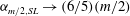Similarly to the other models examined here, the She–Leveque model gives ${\it\alpha}_{1,SL}=0$ and, for $m/2\rightarrow \infty$ , ${\it\alpha}_{m/2,SL}\rightarrow (6/5)(m/2)$ , i.e. for very large $m$ , $\langle {\it\varepsilon}^{m/2}\rangle /\langle {\it\varepsilon}\rangle ^{m/2}$ scales linearly. Therefore, the order-dependent cut-off scales ${\it\eta}_{C,m}/{\it\eta}$ scale as 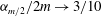${\it\alpha}_{m/2}/2m\rightarrow 3/10$ for large $m/2$ and the She–Leveque model satisfies (4.6), i.e. the cut-off scales remain bounded at finite Reynolds numbers.

The ${\it\alpha}_{m/2}$ as computed from the three models above are shown in figure 4(b). While K62 overpredicts ${\it\alpha}_{m/2}$ as expected, both the p-model and the She–Leveque model are in very good agreement with our DNS. Structure function exponents as computed with (4.5) using the ${\it\alpha}_{m/2}$ from our DNS are shown in table 2, together with the measurements of Anselmet et al. (Reference Anselmet, Gagne and Hopfinger1984) and Gotoh et al. (Reference Gotoh, Fukayama and Nakano2002), which we have averaged when more than one value was reported. While we find very good agreement, it should be kept in mind that the higher orders (for both the measurements of Anselmet et al. (Reference Anselmet, Gagne and Hopfinger1984) and the DNS of Gotoh et al. (Reference Gotoh, Fukayama and Nakano2002) as well as the ones computed from our data) might be subject to significant error bands. It is also worth mentioning that numerical errors in ${\it\alpha}_{m/2}$ translate to smaller errors in ${\it\zeta}_{3(m/2)}$ , at least up to $m/2=4$ . This error decreases with increasing $m/2$ : for instance, ${\it\alpha}_{2}\pm 10\,\%$ yields ${\it\zeta}_{6}\pm 3.77\,\%$ , while ${\it\alpha}_{4}\pm 10\,\%$ yields ${\it\zeta}_{12}\pm 1.16\,\%$ .

5 Resolution requirements

From the existence of scales smaller than the Kolmogorov scale, it follows that this might influence the resolution requirements of DNS, as characterised by the product ${\it\kappa}_{max}{\it\eta}$ , where ${\it\kappa}_{max}$ is the maximum wavenumber resolved by the simulation. Different from earlier work, e.g. by Yakhot & Sreenivasan (Reference Yakhot and Sreenivasan2005), where the multi-fractal model was used to determine the cut-off scales, we use here the exact length scales (3.14). It is therefore worthwhile to examine the required grid resolution in some detail, although it has been studied in the literature by employing different approaches before. Naturally, there is a trade-off for a given number of grid points corresponding to a given ${\it\kappa}_{max}$ between a highly resolved simulation (i.e. a large ${\it\kappa}_{max}{\it\eta}$ ) and a high Reynolds number implying a low ${\it\kappa}_{max}{\it\eta}$ . Common wisdom is to resolve at least $k_{max}{\it\eta}=1$ and usually ${\it\kappa}_{max}{\it\eta}=1.3$ is considered high enough. Note that some studies require a higher resolution, especially if the examined quantities depend on high-order derivatives of the velocity field. An example is the study of Jiménez et al. (Reference Jiménez, Wray, Saffman and Rogallo1993), which required ${\it\kappa}_{max}{\it\eta}=2$ .

It is evident that ${\it\kappa}_{max}{\it\eta}>1$ is needed to resolve the higher moments of the velocity gradient p.d.f., as these are linked to the higher moments of the dissipation. The higher the order of the moment, the higher the necessary resolution. This can also be seen from the data of Ishihara et al. (Reference Ishihara, Kaneda, Yokokawa, Itakura and Uno2007) as well as Donzis et al. (Reference Donzis, Yeung and Sreenivasan2008), where the velocity gradient p.d.f. did not collapse at similar Reynolds number with ${\it\kappa}_{max}{\it\eta}=1$ and ${\it\kappa}_{max}{\it\eta}=2$ ; the dissimilarity is less in the core of the p.d.f. and stronger in the tails, which are determined by the higher moments.

From (3.19), we see that the cut-off lengths ${\it\eta}_{C,m}$ are less resolved for a given ${\it\kappa}_{max}{\it\eta}$ with increasing order $m$ . In order to compare these influences, the normalised resolution

is provided in table 3, where we have used the values of $\langle {\it\varepsilon}^{m/2}\rangle /\langle {\it\varepsilon}\rangle ^{m/2}$ from our data. We also give extrapolated resolutions for $Re_{{\it\lambda}}=10^{3}$ and $Re_{{\it\lambda}}=10^{4}$ , which were computed using the fits shown in figure 4(a). These resolutions are not meant to give exactly the required resolution to resolve the eighth order at $Re_{{\it\lambda}}=10^{3}$ , say, but rather to provide an estimate and to show the influence of the Reynolds number and order. For instance, ${\it\kappa}_{max}{\it\eta}=1.3$ would suggest that the fourth-order structure function (and with it the flatness of the velocity gradient p.d.f.) is completely resolved at $Re_{{\it\lambda}}=10^{4}$ , while higher orders are only partially resolved. Equivalently, we would expect ${\it\kappa}_{max}{\it\eta}=1.3$ at $Re_{{\it\lambda}}=215$ to fully resolve the sixth-order structure function, i.e. this rule of thumb ensures a well enough resolved DNS, if one is interested in lower-order moments at (from the present point of view) low to intermediate Reynolds numbers.

To summarise, if 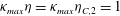${\it\kappa}_{max}{\it\eta}={\it\kappa}_{max}{\it\eta}_{C,2}=1$ completely resolves the second-order structure function, the variance of the velocity gradient p.d.f., the mean dissipation $\langle {\it\varepsilon}\rangle$ and low-order statistics like the mean kinetic energy $\langle k\rangle$ (cf. Yeung & Pope Reference Yeung and Pope1989), then ${\it\kappa}_{max}{\it\eta}_{C,3}=1$ additionally completely resolves the third-order structure function, the skewness of the velocity gradient p.d.f. and the vortex stretching $\langle {\it\omega}_{i}\unicode[STIX]{x1D61A}_{ij}{\it\omega}_{j}\rangle$ , while ${\it\kappa}_{max}{\it\eta}_{C,4}=1$ also resolves the flatness of the velocity gradient p.d.f., the variance of the p.d.f.  $P({\it\varepsilon})$ and the fourth-order structure function, and so on.

Thus, we need more grid points to resolve a certain order when increasing the Reynolds number than the classical estimate using K41 would suggest. There are several estimates of the scaling of numbers of grid points with the Reynolds number – see, for instance, Paladin & Vulpiani (Reference Paladin and Vulpiani1987b ), Davidson (Reference Davidson2004) and Yakhot & Sreenivasan (Reference Yakhot and Sreenivasan2005). In the following, we will use (3.19). If we assume that ${\it\alpha}_{m/2}/(2m)$ converges to a finite number for $m\rightarrow \infty$ , we can use (3.19) to estimate the number of grid points to completely resolve all scales, sometimes also called the number of degrees of freedom of the flow. That is, we can estimate the scaling of grid points with the Reynolds number via

where ${\rm\Delta}x$ is the grid spacing, $L_{Box}$ the length of the DNS box (cube) and $L$ the integral length. Consequently, $N$ is larger than the K41 estimate $N\sim Re_{L}^{9/4}$ since ${\it\alpha}_{m/2}\geqslant 0$ and the scaling of $N$ depends on the asymptotic behaviour of ${\it\alpha}_{m/2}/(2m)$ for $m/2\rightarrow \infty$ . From (4.6), 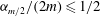${\it\alpha}_{m/2}/(2m)\leqslant 1/2$ (i.e.  ${\it\alpha}_{m/2}/(3m)\leqslant 1/3$ ) and therefore

as upper bound. Paladin & Vulpiani (Reference Paladin and Vulpiani1987b ) used the multi-fractal framework to also obtain $N\sim Re_{L}^{3}$ as the largest Reynolds-number scaling possible (see also Yakhot & Sreenivasan (Reference Yakhot and Sreenivasan2005), where also a $Re_{L}^{3}$ scaling has been found). For the She–Leveque model, ${\it\alpha}_{m/2}/(2m)\rightarrow 3/10$ and one obtains $N\sim Re_{L}^{27/10}$ . Paladin & Vulpiani (Reference Paladin and Vulpiani1987b ) reported $N\sim Re_{L}^{2.3}$ using data from Anselmet et al. (Reference Anselmet, Gagne and Hopfinger1984).