The construction of the claims reserve distribution by means of a semi-Markov backward simulation model

Fulvio Gismondi; Jacques Janssen; Raimondo Manca

doi:10.1017/S1748499511000315

The construction of the claims reserve distribution by means of a semi-Markov backward simulation model

Published online by Cambridge University Press: 09 December 2011

Fulvio Gismondi ,

Jacques Janssen and

Raimondo Manca

Article contents

Abstract
Introduction
The discrete time homogeneous semi-Markov processes
DTHSMP with initial backward recurrence time process
Discounted semi-Markov reward processes with initial backward time
The DTHSMRWP claims reserving model with recurrence backward times
The Monte Carlo DTHSMRWP for the claim reserve distribution construction
An example of claims reserve distribution construction
Conclusions
References

Rights & Permissions

Abstract

The claims reserving problem is currently one of the most debated in actuarial literature. The high level of interest in this topic is due to the fact that Solvency II rules will come into operation in 2014. Indeed, it is expected that quantile computations will be compulsory in the evaluation of company risk and for this reason we think that the construction of the claims reserve random variable distribution assumes a fundamental relevance.

The aim of this paper is to present a method for constructing the claims reserve distribution which can take into account IBNyR (Issued But Not yet Reported) claims in a natural way. The construction of the distribution function for each time of the observed interval is done by means of a Monte Carlo simulation model applied on a backward time semi-Markov process. It should be pointed out that this is the first time that a simulation model based on semi-Markov with backward recurrence time has been presented. The method is totally different from the models given in the current literature.

The most important features given in the paper are:

1) for the first time the Monte Carlo simulation method is applied to a backward semi-Markov environment;

2) the Monte Carlo simulation permits the construction of the random variable of the claims reserve for each year of the studied horizon in a natural way;

3) as already pointed out, the backward process attached to the semi-Markov process permits taking into account the evaluation of the IBNyR claims in a natural way.

In the last part of the paper an applicative example constructed from tables that summarise 4 years of claims from an important Italian insurance company will be given.

Keywords

Semi-Markov processes Stochastic claims reserving backward processes IBNyR claims Monte Carlo simulation

Type: Papers
Information: Annals of Actuarial Science , Volume 6 , Issue 1 , 16 January 2012 , pp. 23 - 64

DOI: https://doi.org/10.1017/S1748499511000315 [Opens in a new window]
Copyright: Copyright © Institute and Faculty of Actuaries 2011

1. Introduction

The claims reserve is the amount that a non-life insurance company should put on its balance sheet taking into account all the claims incurred but not yet, partially or totally, paid. That means forecasting the present value of expenses that derive from both the IBNeR (incurred but not enough reported) claims, (in the sense that they are not yet settled), and the IBNyR (incurred but not yet reported) claims.

Currently, the claims reserve problem is one of the most debated in the actuarial literature concerned with non-life insurance problems. In the first 2009 issue of the ASTIN Bulletin, about 1/3 of the papers were on this topic and, at the moment, any issue of almost any actuarial journal contains at least one paper on this topic.

The relevance of this topic is due to the fact that the Solvency II rules will be applied from January 2014 with an amendment of two months. Rules similar but less demanding were applied in Australia at the beginning of the last decade (Australian Prudential Regulation Authority, 1999). Quantile computations will become compulsory in the evaluation of claims reserve (outstanding liabilities) risk. In this light, it is easy to understand that not only the evaluation of the claims reserve but also the construction of the claims reserve random variable distribution assumes a fundamental relevance.

At first, the claims reserve of insurance companies was evaluated by means of deterministic models like the Chain-Ladder (CL) and the Bornhuetter & Ferguson (BF) (Reference Bornhuetter and Ferguson1972) methods.

As regards these approaches, we recall the Quarg & Mack (Reference Quarg and Mack2004) paper that improved the classical CL model introducing the ratio between the paid and the incurred loss and giving a way to evaluate the IBNyR claims; the Faculty and Institute of Actuaries’ manual (1997); Taylor's book (Reference Taylor2000) and the most recent Wüthrich & Merz (Reference Wüthrich and Merz2008) book in which the deterministic methods for the claims reserve evaluation were described.

Since the end of the eighties, many studies have been dedicated to the construction of the standard deviation error in order to provide a way of measuring risk in the claims-reserving problem.

In this context, we recall the papers by Taylor & Ashe (Reference Taylor and Ashe1983), Ashe (Reference Ashe1986), Renshaw (Reference Renshaw1989), Christofides (Reference Christofides1990), Verrall (Reference Verrall1989, Reference Verrall1990, Reference Verrall1991, Reference Verrall1996, Reference Verrall2000), Wright (Reference Wright1990), Schnieper (Reference Schnieper1991), Mack (Reference Mack1993, Reference Mack1994, Reference Mack1999), Quarg & Mack (Reference Quarg and Mack2004) and more recently, Mack (Reference Mack2008).

Since the second half of the nineties, the claims reserving papers have focused not only on variance computation but also on predicting of the distribution. The first paper in this environment was Wright (Reference Wright1997).

Fundamentally speaking, two approaches were used for the distribution construction, the bootstrapping method and the Markov Chain Monte Carlo (MCMC) method. Two papers, England & Verrall (Reference England and Verrall2002, Reference England and Verrall2006), reported the main results written on these topics. The second paper is by far the most complete due to the fact that it was written four years later and that it is devoted only to these arguments. Furthermore, for a complete bibliography on the distributional methods the interested reader can also refer to the Wüthrich & Merz (Reference Wüthrich and Merz2008) book.

As regards the bootstrap environment, we recall the papers by England & Verrall (Reference England and Verrall1999, Reference England and Verrall2006), England (Reference England2002), Kirschner et al. (Reference Kirschner, Kerley and Isaacs2002), Pinheiro et al. (Reference Pinheiro, Andrade e Silva and de Lourdes Ceneno2003), Taylor & McGuire (Reference Taylor and McGuire2007), Liu & Verrall (Reference Liu and Verrall2009), Bjökwall et al. (Reference Bjökwall, Hössjer and Ohlsson2009) and also the Wüthrich & Merz (Reference Wüthrich and Merz2008) book. In the MCMC case the papers of Haastrup & Arias, Reference Haastrup and Arias1996, de Alba (Reference De Alba2002), England & Verrall (Reference England and Verrall2002, Reference England and Verrall2005, Reference England and Verrall2006), Ntzoufras & Dellaportas (Reference Ntzoufras and Dellaportas2002), Verrall (Reference Verrall2004), Gigante & Sigalotti (Reference Gigante and Sigalotti2005) Merz & Wüthrich (Reference Merz and Wüthrich2006, Reference Merz and Wüthrich2007), Peters et al. (Reference Peters, Shevchenko and Wüthrich2009) and once again the Wüthrich & Merz (Reference Wüthrich and Merz2008) book.

The reported bibliography on this topic is not complete, given the large amount of literature that has been written and the fact that new papers are continually being published. The interested reader can find a good reference list in Schmidt (Reference Schmidt2010).

We should mention that almost all the papers started with the deterministic model and, as a first step, (from the 1980s) these papers tried to introduce risk evaluation by computing the standard deviation error. Subsequently, once the relevance of the distributional methods was understood, the research became devoted to the probability distribution construction of the claims reserve using the bootstrapping or the MCMC methodology but always starting from the CL or BF methods.

Our paper, on the other hand, works with a totally different viewpoint. Firstly, the independence of the cumulative claims of different accident years is supposed, as in all the papers on this topic, and secondly, it is supposed that the evolution of the claim stages

1. IBNyR claims (IBNR),
2. Open Claims (OC),
3. Partially Paid claims (PP),
4. Reopened Claims (RC),
5. Without Payment closed claims (CWP),
6. Closed Claims with payment (PCC),

moves in time following a Discrete Time Homogeneous Semi-Markov Process (DTHSMP). The stages of claims are chosen following the subdivision given in the tables that summarised the situation of the claims of four years of one of the most important Italian insurance companies.

In general non-homogeneity is closer to the real world, but in order to apply it, non-homogeneity needs a lot of data. For example if we have to work in a horizon time of length T and with m states in homogeneous case we have to evaluate T + 1 of m × m order. In the non-homogeneous case we have to evaluate respectively T × (T−1)/2 + T m × m matrices. Non-homogeneity implies a quadratic increasing of the number of variables that should be evaluated, the homogeneity a linear increasing. This is the main reason why it is difficult to apply non-homogeneous models in a real world application. Furthermore, in the case of claims we think that the duration inside the states does not depend greatly on the starting time because it depends, rather, on the behaviour of the people that have to manage the claim. Fundamentally, the waiting time depends on the insured person taking time to report the claim, the insurer taking time to pay, the judgment that can have a random duration and so on. We think that none of these times depends on the moment in which the claim happened. These are the reasons whereby we choose to construct a homogeneous model.

Homogeneous semi-Markov Processes (HSMP) were defined independently by Levy (Reference Levy1954), Smith (Reference Smith1954) & Takacs (Reference Takacs1954). DTHSMP and its numerical solution were described in De Dominicis & Manca (Reference De Dominicis and Manca1984a) and successively in Corradi et al. (Reference Corradi, Janssen and Manca2004) and Barbu et al. (Reference Barbu, Boussemart and Limnios2004). A complete description of homogeneous SMP both in continuous and discrete time environment can be found in Janssen & Manca (Reference Janssen and Manca2006 and Reference Janssen and Manca2007). Applications of the semi-Markov processes in insurance were presented, for example, in Janssen (Reference Janssen1966), Hoem (Reference Hoem1972), Janssen & De Dominicis (Reference Janssen and De Dominicis1984), De Dominicis & Manca (Reference De Dominicis and Manca1984b), Balcer & Sahin (Reference Balcer and Sahin1986), De Medici et al. (Reference De Medici, Janssen and Manca1995), Janssen & Manca (Reference Janssen and Manca1997), Haberman & Pitacco (Reference Haberman and Pitacco1999), Stenberg et al. (Reference Stenberg, Manca and Silvestrov2006, Reference Stenberg, Manca and Silvestrov2007), Janssen & Manca (Reference Janssen and Manca2007), D'Amico et al. (Reference D'Amico, Guillen and Manca2009).

In Norberg (Reference Norberg1993, Reference Norberg1999) four stages were defined

1. Covered not incurred,
2. Incurred not reported,
3. Reported not settled,
4. Settled.

that are in time sequence. It should be pointed out that the stage covered–not-incurred in the claim reserving evaluation does not make sense because only the incurred claims should be taken into consideration. The trajectory among the other three stages is not random. The randomness is given by the waiting time inside the states and it is modeled by a non-homogeneous marked Poisson process. Our model, that is in a discrete time environment has two randomness, time and the transitions between the stages. Furthermore, Poisson processes suppose a time evolution modeled by negative exponential distribution functions (d.f.) in continuous time case and geometric in the discrete time case whereas the waiting time d.f. in a SMP can be managed by any type of parametric and also non-parametric distribution.

Another paper (Hesselager (Reference Hesselager1994)) presented a model in which the stages of the claims are states of a non-homogeneous continuous time Markov process. In some senses this paper generalized the model presented in Norberg (Reference Norberg1993). In Hesselager's paper the states are the same of the ones given in Norberg's paper. A new state is introduced only by dividing the Reported But Not Settled claims in two parts; the subdivision is, therefore, a function of the claim cost. Firstly, we have to recall that in continuous time Markov processes waiting time distribution functions are negative exponential and it is very unlikely that this happens in real problems. Finally it should also be pointed out that, in our model, the “delay times” due to IBNyR claims are considered in a natural way in a discrete time environment too.

The approach of this paper is new because a Monte Carlo semi-Markov model with backward recurrence time has never been applied. In Biffi et al. (Reference Biffi, Janssen and Manca2007), the idea of constructing the claims reserving by means of a Monte Carlo DTHSMP was presented. The paper was, fundamentally, a simple explanation of the idea. The IBNyR claims were not considered in that paper given the lack of backward recurrence time. In Biffi et al. (Reference Biffi, D'Amico, Di Biase, Janssen, Manca and Silvestrov2008a, Reference Biffi, D'Amico, Di Biase, Janssen, Manca and Silvestrov2008b) the same idea was applied in a credit risk environment and the backward processes were not applied in this paper either. Furthermore, this approach is totally different from the claims reserve stochastic models of other authors.

The main contributions of this paper are that:

1) the Monte Carlo simulation method has been applied to a backward semi-Markov environment for the first time;
2) the Monte Carlo simulation permits the construction of the random variable of the claims reserve for each year of the studied horizon in a natural way;
3) the backward process attached to the semi-Markov process permits evaluation of the IBNyR claims to be taken into account in a natural way.

In section 2, a brief introduction to the discrete time homogeneous SMP is given. Section 3 presents the DTHSMP with attached a backward time process (see Silvestrov, Reference Silvestrov1980) and, more recently, Limnios & Oprişan, Reference Limnios and Oprişan2001 and Janssen & Manca, Reference Janssen and Manca2006). This section will show how the backward recurrence time process attached to a DTHSMP allows the problem of the forecasting of IBNyR to be solved in a natural way. In section 4 a quick introduction to DTHSMP with reward is given. Section 5 describes how the claims reserve problem can be solved by means of DTHSMP. Section 6 explains how the claims reserve stochastic process evolution can be constructed by means of the Monte Carlo simulation model applied to a DTHSMP with backward recurrence time. Section 7 reports a real data example. Some conclusions close the paper.

2. The discrete time homogeneous semi-Markov processes

On a complete probability space (Ω, $)(--><$>\scr F <$><$>{{J}_n},\,\,\,n\: \in \:{\Bbb N} <$><$>{{T}_n},\,\,\,n\: \in \:{\Bbb N}, <$><$>{\Bbb N} <$><!--$ and representing the time of the n-th transition.

$--><$$>{{J}_n}:\Omega \rightarrow E\; \; {{T}_n}:\Omega \rightarrow {\Bbb N}.\eqno<$$><!--$

The process (J_n,T_n) is a homogeneous Markovian renewal process if its kernel

$--><$$> {\bf {{Q}}}\: = \:\left[ {{{Q}_{ij}}(t)} \right] \eqno<$$><!--$

satisfying the following property:

(2.1)

$--><$$> \eqalign{ {{Q}_{ij}}(t)\: \equiv \: & {\rm{P}}\left[ {{{J}_{n\: + \:1}}\: = \:j,\,{{T}_{n\: + \:1}}{\rm{ - }}{{T}_n}\:\leq \:t|\,{{J}_n}\: = \:i,\,\,({{J}_\nu },{{T}_\nu }),\,0\:\leq \:\nu \: \lt \:n} \right] \cr & = \:{\rm{P}}\left[ {{{J}_{n\: + \:1}}\: = \:j,\,{{T}_{n\: + \:1}}{\rm{ - }}{{T}_n}\:\leq \:t|\,{{J}_n}\: = \:i} \right]. \cr} \eqno<$$><!--$

Remark 1: In the claims reserve problem the states of the system are the stages of the incurred claims. Under the SMP hypotheses it results that the future of the system (stages evolution) depends only on the present. The past history is cancelled. □

It results that:

(2.2)

$--><$$> {{p}_{ij}}\: \equiv \:{\rm{P}}\left[ {{{J}_{n\: + \:1}}\: = \:j|{{J}_n}\: = \:i} \right]\: = \:{\mathop{{\lim }}\limits_{{t \rightarrow \infty }}} {{Q}_{ij}}(t);\,\,\,i,j\: \in \:E,\,\,t\: \in \:{\Bbb N}, \eqno<$$><!--$

The matrix P = [p_ij] expresses the transition probability matrix of the embedded homogeneous Markov chain.

Furthermore it is necessary to introduce the probability that the process will have a transition from state i within a time t:

$--><$$> {{H}_i}(t)\: \equiv \:{\rm{P}}\left[ {\,{{T}_{n\: + \:1}}{\rm{ - }}{{T}_n}\:\leq \:t|\,{{J}_n}\: = \:i} \right]\: = \:\mathop{\sum}\limits_{j\: \in \:E} {{{Q}_{ij}}(t)} . \eqno<$$><!--$

If i is not an absorbing state, it is clear that

$--><$$> {\mathop{{\lim }}\limits_{{t \rightarrow \infty }}} {{H}_i}(t)\: = \:1. \eqno<$$><!--$

Furthermore, the following probabilities are considered:

$--><$$> {{b}_{ij}}(t)\: = \:{\rm{P}}\left[ {{{J}_{n\: + \:1}}\: = \:j,\,{{T}_{n\: + \:1}}{\rm{ - }}{{T}_n}\: = \:t|\,{{J}_n}\: = \:i} \right]. \eqno<$$><!--$

These probabilities can be given in function of the Q_ij(t):

$--><$$> {{b}_{ij}}(t)\: = \:\left\{ {\matrix{ {{{Q}_{ij}}(0)\: = \:{\rm{0}}\,\,\,{\rm{if}}\,\,\,t\: = \:0} \hfill\cr {{{Q}_{ij}}(t){\rm{ - }}{{Q}_{ij}}(t{\rm{ - }}1)\,\,\,\,{\rm{if}}\,\,t\: = \:1,2,\, \ldots } \right \eqno<$$><!--$

Now it is possible to define the distribution functions (d.f.) of the waiting time in each state i, given that the state j successively occupied is known:

$--><$$> {{F}_{ij}}(t)\: = \:{\rm{P}}\left[ {\,{{T}_{n\: + \:1}}{\rm{ - }}{{T}_n}\:\leq \:t|\,{{J}_n}\: = \:i,{{J}_{n\: + \:1}}\: = \:j} \right]. \eqno<$$><!--$

These probabilities can be obtained by means of the following formula:

$--><$$> {{F}_{ij}}(t){}\: = \:{}\left\{ {\matrix{ {{{Q}_{ij}}(t) / {{p}_{ij}}} & {{\rm{if}}} & {{{p}_{ij}}\: \ne \:0} \cr 1 & {{\rm{if}}} & {{{p}_{ij}}\: = \:0.} \right \eqno<$$><!--$

Defining N(t) = sup{n|T_n ≤ t}, $)(--><$>\forall t\: \in \:{\Bbb N}<$><$>Z\: = \:\left( {Z(t),\,\,t\: \in \:{\Bbb N}} \right)<$><!--$ can be defined, as Z(t) = J_N ₍_t ₎, representing, for each waiting time, the state occupied by the process.

The semi-Markov process transition probabilities are defined in the following way:

$--><$$> {{\phi }_{ij}}(t)\: = \:{\rm{P}}\left[ {Z(t)\: = \:j|Z(0)\: = \:i} \right]. \eqno<$$><!--$

Remark 2: In a homogeneous environment the time represents the duration after a given transition. So the elements of couple (T_n, J_n) represents respectively the time and the state of the n-th transition. If we wish to follow the system after this transition if J_n = i then the duration time begins from 0, T_N ₍₀₎ = T_n and Z(0) = i. □

The φ_ij(t) are obtained by solving the following evolution equations:

(2.3)

$--><$$> {{\phi }_{ij}}(t)\: = \:{{\delta }_{ij}}(1{\rm{ - }}{{H}_i}(t))\: + \:\mathop{\sum}\limits_{\beta \in E} {\mathop{\sum}\limits_{\vartheta \: = \:1}^t {{{b}_{i\beta }}(\vartheta ){{\phi }_{\beta j}}(t{\rm{ - }}\vartheta )} } \eqno<$$><!--$

where δ_ij represents the Kronecker symbol.

φ_ij(t) represents the probability of remaining in state j at time t, given that at time 0 the system entered state i.

Remark 3: If the p_ij and the F_ij(t) are known then it is possible to solve (2.1) obtaining the Q_ij(t). From the Q_ij(t) the b_ij(t) and the H_i(t) can be obtained and in this way (2.3) can be solved. □

In the first part of formula (2.3) the 1−H_i(t) gives the probability of the system not having transitions up to the time t given that it entered the state i at time 0. The 1−H_i(t) in our insurance model represents the probability that our system does not change stage within the time t. This part makes sense if and only if i = j.

In the second part of (2.3), b_iβ(ϑ) represents the probability of the system entering state β just at time ϑ given that it entered state i at time 0 (homogeneous behaviour). After the transition, the system will go to state j following one of the possible trajectories that go from state β in a time ϑ and bring the system to state j at time t.

There are well known algorithms which make the solution of equation possible (2.3), see for example Janssen & Manca (Reference Janssen and Manca2007).

3. DTHSMP with initial backward recurrence time process

Definition 1: Let B(t) = t−T_N ₍_t ₎ be the backward recurrence time process in a semi-Markov environment. It represents the difference between the observation time t and the time of the last transition. (see Limnios & Oprişan, Reference Limnios and Oprişan2001, Janssen & Manca, Reference Janssen and Manca2006). □

Remark 4: The concept of backward time is very easy to understand. Imagine that a person goes to a bus station then the elapsed time between the arrival of the last bus and the arrival of the person is a backward time. In non-life insurance the time between the moment in which the claims occurred and the time in which it was reported is another example of backward time.

Then we define the following probability:

(3.1)

$--><$$>{\pre}^{b}{{\phi }_{ij}}(l;t)\: = \:{\rm{P}}\left[ {Z(t)\: = \:j|\,Z(0)\: = \:i,\,B(0)\: = \:l} \right],\eqno<$$><!--$

where (3.1) represents the semi-Markov transition probabilities with initial backward recurrence time.

Remark 5: As pointed out in Remark 2, if the system is followed after the n-th transition, this time with a backward recurrence time l, the system is in state i (Z(0) = i) but the transition in i happened l periods before. We know also that, taking into account the duration time, it entered this state at time −l where l represents the initial backward time (see Figure 1). (3.1) gives the probability of being in state j at time t. □

Figure 1 HSMP with backward time trajectory

In Figure 1 a trajectory of an HSMP with initial backward recurrence time is reported. In a homogeneous environment the system starts from time 0. We have that N(0) = n, because we start to follow our system after the n-th transition. The starting backward is B(0) = l then T_n = −l represents, in function of homogeneous hypothesis, the time of the n-th transition and J_n the related state. The time t represents the duration from 0. J_h ₋₁ = j the state of the h−1-th transition, T_h ₋₁ the time of arrival in the state j and N(t) = h−1, h−1 > n.

To present the evolution equations of probabilities (3.1) we introduce the following notation:

(3.2)

$--><$$> {{D}_i}(l;t)\: = \:\frac{{1{\rm{ - }}{{H}_i}(l\: + \:t)}}{{1{\rm{ - }}{{H}_i}(l)}} \eqno<$$><!--$

which represents the probability of having no transition from state i between times −l and t given that no transition occured from state i between times −l and 0.

Moreover by

(3.3)

$--><$$>{{ b}_{ij}}(l;t)\: = \:\frac{{{{b}_{ij}}(l\: + \:t)}}{{1{\rm{ - }}{{H}_i}(l)}}\eqno<$$><!--$

we denote the probability of making the next transition from state i to state j just at time t given that the system does not make transitions from state i between times −l and 0.

The relation (3.4) represents the evolution equations of (3.1)

(3.4)

$--><$$> {\pre}^{b}{{\phi }_{ij}}(l;t)\: = \:{{D}_i}(l;t)\: + \:\mathop{\sum}\limits_{\beta \: \in \:E}^{} {\mathop{\sum}\limits_{\vartheta \: = \:s\: + \:1}^t {{{b}_{i\beta }}(l;\vartheta ){{\phi }_{\beta j}}(t{\rm{ - }}\vartheta )} }, \eqno<$$><!--$

Remark 6: As results from (3.2) and (3.3), the initial data necessary to solve the evolution equation (3.4) are the same as those necessary to solve relation (2.3). The introduction of backward recurrence times gives greater information on the studied system without the necessity of new statistical data. □

Remark 7: According to our assumptions, if we constructed the Q_ij(t) correctly, then the conditioned probabilities (3.2) and (3.3) take into account, by definition, the non-movement from the state i for a time l. The (3.4) solution gives the probabilities of being in state j at time t given that the observed system was in the state i at time 0 and given that it has been in this state from a time l. The IBNyR represents this kind of situation. For example, if an accident occurred at time s and it was reported at time s + l, then l will be a backward time. Our model permits the consideration of the time before the reporting of the accident in a natural way. □

4. Discounted semi-Markov reward processes with initial backward time

Now we introduce the reward structure. A permanence (or rate) reward ψ_i(t) is paid or received for the permanence in the state i. The process stays in the state i at the time t and for his stay the reward is given for an insurance contract starting at time 0. An impulse (or transition) reward γ_ij(t) is paid due to the transition from state i to state j at time t for a contract starting at time 0. The permanence reward can be seen as an annuity-type payment and it can be a positive or a negative sum. The impulse reward can be seen as a lump-sum payment. We assume that permanence and impulse rewards are sums of money that have to be discounted using a discrete time discount factor ν(t).

Following the line of research of Stenberg et al. (Reference Stenberg, Manca and Silvestrov2006) we define the accumulated reward process by means of the following relation:

Definition 2: Let ξ_i(t) be the stochastic process that represents the discounted accumulated Discrete Time Homogeneous Semi-Markov ReWard Process (DTHSMRWP) starting at time 0 from the state i, defined at time t by

(4.1)

$--><$$>\matrix{ {{\xi }_i}\left( t \right)\: = \:\chi \left( {{{T}_{N(0)\: + \:1}}\: \gt \:t|{{J}_{N(0)}}\: = \:i,{{T}_{N(0)}}\: = \:0} \right)\mathop{\sum}\limits_{\tau \: = \:1}^t {{{\psi }_i}(\tau ) \nu (\tau )} \hfill \cr \quad\qquad+ \mathop{\sum}\limits_{k \in E} {\mathop{\sum}\limits_{\theta \: = \:1}^t {\chi \left( {{{J}_{N(0)\: + \:1}} = k,{{T}_{N(0)\: + \:1}}\: = \:\theta |{{J}_{N(0)}}\: = \:i,{{T}_{N(0)}}\: = \:0} \right)} } \hfill\cr \ \qquad \zrad \left( {\mathop{\sum}\limits_{\tau \: = \:1}^{{{T}_{N(0)\: + \:1}}} {{{\psi }_i}(\tau ) \nu (\tau )\: + \:{{\gamma }_{i,{{J}_{N(0)\: + \:1}}}}\left( {{{T}_{N(0)\: + \:1}}} \right)\nu({{T}_{N(0)\: + \:1}})\: + \:{{\xi }_{{{J}_{N(0)\: + \:1}}}}\left( {t{\rm{ - }}{{T}_{N(0)\: + \:1}}} \right) \nu ({{T}_{N(0)\: + \:1}})} } \right), \eqno<$$><!--$

where:

1) $)(--><$>\chi (a)\: = \:\left\{ {\matrix{ 1 & {{\rm{if \ the \ event \ }} a \ {\rm{ is \ verified}}} \cr 0 & {{\rm{if \ the \ event }} \ a \ {\rm{ is \ not \ verified}}} \right <$><!--$
2) T_N ₍₀₎ represents the random time of the n-th transition and T_N _{(0) + 1} the random time of the n + 1-st transition. □

If we denote by V_i(t) = E[ξ_i(t)], by taking the expectation of (4.1) we have

(4.2)

$--><$$>V_{i}^{{}} \left( t \right)\: = \:(1{\rm{ - }}{{H}_i}(t))\mathop{\sum}\limits_{\tau \: = \:1}^t {{{\psi }_i}(\tau ) \nu (\tau )} \: + \:\mathop{\sum}\limits_{k\: \in \:E} {\mathop{\sum}\limits_{\theta \: = \:1}^t {{{b}_{ik}}\left( \theta \right)} } \zrad \left( {\mathop{\sum}\limits_{\tau \: = \:1}^\theta {{{\psi }_i}(\tau ) \nu (\tau )\: + \:{{\gamma }_{i,k}}\left( \theta \right) \nu (\theta )\: + \:{{V}_k}\left( {t{\rm{ - }}\theta } \right) \nu (\theta )} } \right).\eqno<$$><!--$

where θ represents the possible values that the r.v. T_N _{(0) + 1} can assume within the time t.

The mean present value given by (4.2) can be subdivided into 4 parts:

(4.3)

$--><$$>(1{\rm{ - }}{{H}_i}(t))\mathop{\sum}\limits_{\tau \: = \:1}^t {{{\psi }_i}(\tau ) \nu (\tau )}, \eqno<$$><!--$

(4.4)

$--><$$>{{b}_{ik}}\left( \theta \right)\zrad \mathop{\sum}\limits_{\tau \: = \:1}^\theta {{{\psi }_i}(\tau ) \nu (\tau )}, \eqno<$$><!--$

(4.5)

$--><$$>{{b}_{ik}}\left( \theta \right)\zrad {{\gamma }_{i,k}}\left( \theta \right) \nu (\theta ),\eqno<$$><!--$

(4.6)

$--><$$>{{b}_{ik}}\left( \theta \right)\zrad {{V}_k}\left( {t{\rm{ - }}\theta } \right) \nu (\theta ),\eqno<$$><!--$

(4.3) gives the mean present value of the permanence rewards that are obtained if there are no transitions from the state i up to time t

b_ik(θ) means that the system had a transition into state k exactly at time θ. (4.4) gives the mean present value of the permanence rewards that is obtained by remaining in the state i up to the time θ.

(4.5) gives the mean present value of the impulse reward that is obtained because of the transition from the state i to the state k at time θ.

(4.6) gives the mean present value of all the rewards that were obtained in a time t−θ starting from the state k. This amount must be discounted at time 0.

Definition 3: Let ξ_i(l;t) be the discounted accumulated DTHSMRWP with initial backward time, defined by

(4.7)

$--><$$>\openup 6pt\matrix{ {\pre}^{b}\xi _{i}^{{}} \left( {l;t} \right)\: = \:\chi \left( {{{T}_{N(0)\: + \:1}}\: \gt \:t|{{J}_{N(0)}}\: = \:i,{{T}_{N(0)}}\: = \:{\rm{ - }}l,{{T}_{N(0)\: + \:1}}\: \gt \:0} \right)\mathop{\sum}\limits_{\tau \: = \:1}^t {{{\psi }_i}(\tau ) \nu (\tau )} \hfill\cr \qquad \qquad+ \mathop{\sum}\limits_{k \in E} {\mathop{\sum}\limits_{\theta \: = \:1}^t {\chi \left( {{{J}_{N(0)\: + \:1}}\: = \:k,{{T}_{N(0)\: + \:1}}\: = \:\theta |{{J}_{N(0)}}\: = \:i,{{T}_{N(0)}}\: = \:{\rm{ - }}l,{{T}_{N(0)\: + \:1}}\: \gt \:0} \right)} \cdot } \hfill\cr \qquad \qquad\left( {\mathop{\sum}\limits_{\tau \: = \:1}^{{{T}_{N(0) + 1}}} {{{\psi }_i}(\tau ) \nu (\tau )\: + \:{{\gamma }_{i,{{J}_{N(0)\: + \:1}}}}\left( {{{T}_{N(0)\: + \:1}}} \right) \nu ({{T}_{N(0)\: + \:1}})\: + \:{{\xi }_{{{J}_{N(0)\: + \:1}}}}\left( {t{\rm{ - }}{{T}_{N(0)\: + \:1}}} \right) \nu ({{T}_{N(0)\: + \:1}})} } \right). \eqno<$$><!--$

If we denote by $)(--><$>V_{i}^{b} \left( {l;t} \right)\: = \:E\left[ {\xi _{i}^{b} \left( {l;t} \right)} \right] <$><!--$ , by taking the expectation of (4.7) we have

(4.8)

$--><$$>{\pre}^{b}V_{i}^{{}} \left( {l;t} \right)\: = \:{{d}_i}(l;t)\left( {\mathop{\sum}\limits_{\tau \: = \:1}^t {{{\psi }_i}(\tau ) \nu (\tau )} } \right)\: + \:\mathop{\sum}\limits_{k\: \in \:E} {\mathop{\sum}\limits_{\theta \: = \:1}^t {{{b}_{ik}}\left( {l;\theta } \right)} \zrad } \left( {\mathop{\sum}\limits_{\tau \: = \:1}^\theta {{{\psi }_i}(\tau ) \nu (\tau )\: + \:{{\gamma }_{i,k}}\left( \theta \right) \nu (\theta )\: + \:{{V}_k}\left( {t{\rm{ - }}\theta } \right) \nu (\theta )} } \right).\eqno<$$><!--$

The (4.8) relation is a general relation that gives the mean present value of the rewards that were paid in the horizon time that was followed by (4.8). It is possible to obtain different relations depending on the case study (see Janssen & Manca, Reference Janssen and Manca2007). □

Remark 8: The DTHSMRWP is a class of processes. The evolution equation changes if we have only permanence rewards or only transition rewards; it changes if we have fixed or variable interest rate. There are DTHSMRWP without discount factors and so on. Non-life insurance includes health insurance contracts and also accident insurance and it is possible to have both permanence and transition rewards. In our case we will present an example to motor insurance. In this case the DTHSMRWP model will be discounted and without the permanence rewards. □

In this case the evolution equation (4.8) will assume the following form

(4.9)

$--><$$>{\pre}^{b}V_{i}^{{}} \left( {l;t} \right)\: = \:\mathop{\sum}\limits_{k\: \in \:E} {\mathop{\sum}\limits_{\theta \: = \:1}^t {{{b}_{ik}}\left( {l;\theta } \right)} \zrad } \left( {{{\gamma }_{i,k}}\left( \theta \right) \nu (\theta )\: + \:{{V}_k}\left( {t{\rm{ - }}\theta } \right) \nu (\theta )} \right).\eqno<$$><!--$

Following the approach of Stenberg et al. (Reference Stenberg, Manca and Silvestrov2006) and particularising at our case, it is possible to derive recursive equations for the higher order moments of the reward processes ξ_i(l;t). For example, the second moment of the (4.9) is given by:

(4.10)

$--><$$>\matrix{ \openup 6pt{{\left( {{\pre}^{b}V_{i}^{{}} \left( {l;t} \right)} \right)}^{(2)}} \: = \:\mathop{\sum}\limits_{k\: \in \:E} {\mathop{\sum}\limits_{\theta \: = \:1}^t {{{b}_{ik}}\left( {l;\theta } \right)} \zrad {{{\left( {{{\gamma }_{i,k}}\left( \theta \right) \nu (\theta )} \right)}}^2} } \: + \:2\mathop{\sum}\limits_{k\: \in \:I} {\mathop{\sum}\limits_{\theta \: = \:1}^t {{{b}_{ik}}\left( {l;\theta } \right)} {{\gamma }_{i,k}}\left( \theta \right) \nu (\theta ){{V}_k}\left( {t{\rm{ - }}\theta } \right)} \cr + \mathop{\sum}\limits_{k\: \in \:I} {\mathop{\sum}\limits_{\theta \: = \:1}^t {{{b}_{ik}}\left( {l;\theta } \right)} \zrad {{{\left( {{{V}_k}\left( {t{\rm{ - }}\theta } \right)} \right)}}^{(2)}} {{{\left( {\nu(\theta )} \right)}}^2} } . \eqno<$$><!--$

Once the (4.9) and (4.10) evolution equations are solved, clearly it is possible to compute the variance and the standard deviations.

The other higher order moments can be obtained by means of the general relations given in Stenberg et al. (Reference Stenberg, Manca and Silvestrov2006).

Remark 9: Our equations (4.9) and (4.10) make provision in a complete and natural way for the time spent in a state before we begin to follow the system. Indeed the backward recurrence time process attached to the DTHSMRWP offers this opportunity. □

5. The DTHSMRWP claims reserving model with recurrence backward times

Once a claim occurs it can be reported (OC) or not reported (IBNyR). In the stage of not being reported it can wait for a random time before it is finally reported. In the same way, a reported claim can be partially or totally paid or closed without payments and, in this case too, the waiting time inside the state (OC) is a random variable (r.v.). It is very important to consider the duration inside the claims stages in a thorough way. This can be done by means of the backward time processes.

Furthermore, if we work according to the Markovian hypothesis (the future depends only on the present), and take into account the fact that the transitions between the claims stages depend on the starting and on the arriving stages, then we can suppose that the stage represents the state of a system that evolves under a DTHSMP to which a backward time process is attached.

To re-cap by means of backward time, it is possible to consider, and in a natural way, the time spent in a stage before the transition to another stage.

To solve the evolution equation of a DTSMP it is necessary to construct the embedded MC P and the matrix of the conditioned waiting time distribution functions F(t),t = 1,…,T where T is the time horizon in which the studied system will be followed.

The non-parametric P and the F constructions are very simple if there are the raw data. As results from (2.2) P is a limit at +∞ and for its computation we should consider all the transitions that will happen in [0, T]. The F construction can be done simultaneously with the P. Indeed, for each i, j we can construct a frequency time vector $)(--><$>{{{ {{\bar {\bf f}}}}}_{ij}}\: = \:\left\{ {{{{\bar{f}}}_{ij}}(t),\,t\: = \:1, \ldots, T} \right\} <$><!--$ . In each element of this vector the transition number that happened just at time t will be stored. Dividing the elements of this vector by p_ij and recursively summing the previous element to the subsequent a non-parametric conditioned waiting time distribution function (d.f.) is obtained.

It is clear that T could not cover all the time in which the studied phenomenon makes sense. In this case we have to use a truncated d.f. The truncation could be done taking into account past experiences.

In the claims reserve case, supposing a time interval of at least 20 years, it will be possible to avoid the d.f. truncation because it is reasonable to assume that 20 years are sufficient to close any occurred claims.

Example 1: The construction of P and F. We suppose that T = 4, m = 3 and that we know that the studied phenomenon never can wait inside a state more than 4 time periods. From raw data we obtain the following matrices:

$--><$$> \eqalign{ {{{\bar{\bf P}}}}\: = \:\left[ {\matrix{ {48} & {201} & {123} \cr {32} & {154} & {211} \cr {85} & {302} & {288} }}\right]; \,\,\,{\bf {{N}}}\: = \:\left[ {\matrix{ {372} \cr {397} \cr {675} }}\right];\,\,\,{\bf {{P}}}\: = \:\left[ {\matrix{ {.129} & {.540} & {.331} \cr {.081} & {.388} & {.531} \cr {.126} & {.447} & {.427} }} \right] \cr & {{{\bar{\bf F}}}}\: = \:\left[ {\matrix{ {\left[ {\matrix{ {13} & {45} & {22} \cr 8 & {28} & {75} \cr {12} & {88} & {89} }}} \right]} & {\left[ {\matrix{ 4 & {62} & {17} \cr 9 & {31} & {28} \cr {23} & {26} & {57} }} \right]} & {\left[ {\matrix{ {20} & {54} & {42} \cr {11} & {44} & {47} \cr {18} & {118} & {98} }} \right]} & {\left[ {\matrix{ {11} & {40} & {42} \cr 4 & {51} & {61} \cr {32} & {70} & {44} }} \right]} }}}} \right] \cr \left{{{{{ {{{\tilde{\bf F}}}}\: = \:\left[ {\matrix{ {\left[ {\matrix{ {.271} & {.224} & {.178} \cr {.25} & {.182} & {.355} \cr {.141} & {.291} & {.309} }}\right]} & {\left[ {\matrix{ {.083} & {.308} & {.138} \cr {.281} & {.201} & {.133} \cr {.271} & {.086} & {.198} }}\right]} & {\left[ {\matrix{ {.417} & {.269} & {.342} \cr {.344} & {.286} & {.223} \cr {.212} & {.391} & {.340} }} \right]} & {\left[ {\matrix{ {.229} & {.199} & {.342} \cr {.125} & {.331} & {.289} \cr {.376} & {.232} & {.153} }} \right]} }} \right} }}}} \right] \cr \left{{{{{ {\bf {{F}}}\: = \:\left[{\matrix{ \left[ {{\matrix {{.271} & {.224} & {.178} \cr {.25} & {.182} & {.355} \cr {.141} & {.291} & {.309} }}}\right]} & {\left[ {\matrix{ {.354} & {.532} & {.316} \cr {.531} & {.383} & {.488} \cr {.412} & {.377} & {.507} }} \right]} & {\left[ {\matrix {{.771} & {.801} & {658} \cr {.875} & {.669} & {.711} \cr {.624} & {.768} & {.847} }} \right]} & {\left[ {\matrix{ 1 & 1 & 1 \cr 1 & 1 & 1 \cr 1 & 1 & 1 }}\right]} }\right]. \eqno<$$><!--$

In the matrix $)(--><$>{{{\bar{\bf P}}}} <$><$>{{\bar{p}}_{23}}\: = \:211 <$><$> {{{{{\bar{\bf f}}}}}_{2,3}}\: = \:[{{\bar{f}}_{2,3}}(1),{{\bar{f}}_{2,3}}(2),{{\bar{f}}_{2,3}}(3),{{\bar{f}}_{2,3}}(4)]\: = \:[75,28,47,61] <$><$>{{{ {{\tilde{\bf f}}}}}_{2,3}}\: = \:[0.{\rm{355}},{}0.{\rm{133}},{}0.{\rm{223, }}0.{\rm{289]}} <$><!--$ is the vector of the probabilities that a transition from the state 2 to state 3 will happen in the first, the second, the third and the fourth year.

As can be easily understood, the elements of matrix F represent the waiting time d.f. and are obtained by summing the corresponding elements of the four sub-matrices of the matrix $)(--><$>{{{\tilde{\bf F}}}}. <$><!--$ □

Once the P and F are constructed, it will be possible to solve (4.9) and (4.10) and, if necessary, to compute also the skewness and the kurtosis (see Stenberg et al., Reference Stenberg, Manca and Silvestrov2006). These results are obtained for each starting state, for each year of the time horizon and for each backward time. This means that we can take into account, the IBNyR and of IBNeR claims, again in a natural way, by considering the time at which the claims arrived in the stage.

If we were only looking for the results that can be obtained solving our SMP we could stop here, but we are also interested in the distributional study of the claim reserving process for the given time horizon so we need another approach to solve the problem.

6. The Monte Carlo DTHSMRWP for the claim reserve distribution construction

6.1 The claim reserve construction

Our aim is to construct the distribution of the claims reserve and it will be carried out by means of a Monte Carlo simulation method applied to our DTHSMRWP with backward recurrence time. We should mention that this is the first time that a simulation SMP with backward time has been presented.

The first paper that introduced a real life Monte Carlo HSMP simulation model in the context of the claims reserving problem was Biffi et al. (Reference Biffi, Janssen and Manca2007). Another paper, which was divided into two parts, Biffi et al. (Reference Biffi, D'Amico, Di Biase, Janssen, Manca and Silvestrov2008a, Reference Biffi, D'Amico, Di Biase, Janssen, Manca and Silvestrov2008b) proposed a Monte Carlo non-homogeneous SMP model in a credit risk environment.

To apply the Monte Carlo simulation method it is necessary to compute the P and F matrices and begin the simulation as is described in Limnios & Oprişan (Reference Limnios and Oprişan2001). More precisely, it is possible to construct a trajectory of the process starting at time 0 from the state i in two steps:

– extracting a pseudorandom number that gives the arriving state of the transition taking into account the probability distribution p_ij, j ∈ E,
– extracting another pseudorandom number that gives the time t of the transition considering the conditioned waiting time d.f. F_ij(t), t = 1,…,T.

We choose the second way of constructing the trajectory. Our simulation model obtains the time t from the first construction of a pseudorandom number by means of the H_i(t) values and the state j from the second construction that can be obtained by the following probability function:

(6.1)

$--><$$>\frac{{b_{{ij}}^{{}} (t)}}{{H_{i}^{{}} (t){\rm{ - }}H_{i}^{{}} (t{\rm{ - }}1)}}\: = \:{\rm{P}}\left[ {{{J}_{n\: + \:1}}\: = \:j|{{J}_n}\: = \:i,{{T}_{n\: + \:1}}{\rm{ - }}{{T}_n}\: = \:t} \right].\eqno<$$><!--$

Indeed, it results:

$--><$$>\mathop{\sum}\limits_{j\: \in \:E}^{} {\frac{{b_{{ij}}^{{}} (t)}}{{H_{i}^{{}} (t){\rm{ - }}H_{i}^{{}} (t{\rm{ - }}1)}}} \: = \:1\eqno<$$><!--$

We prefer this second way because by extracting the time t, if t is outside of our time horizon T, we can avoid looking for the state of the related transition. In this way it is possible to avoid one pseudorandom number extraction for the studied trajectory. Taking into account that in the example that we will present in the next section we constructed 122,000,000 trajectories the relevance of this fact can be understood.

Remark 10: H_i(t) and (6.1) hold in the DTHSMP without backward time. The corresponding elements in DTHSMP with backward time can be constructed in the following way:

(6.2)

$--><$$> \,{{H}_i}(l;t)\: = \:\frac{{{{H}_i}(l\: + \:t)}}{{1{\rm{ - }}{{H}_i}(l)}}, \eqno<$$><!--$

(6.3)

$--><$$> \,{{\bar{b}}_{ij}}(l;t)\: = \:\frac{{{{b}_{ij}}(l;t)}}{{{{H}_i}(l;t){\rm{ - }}{{H}_i}(l;t{\rm{ - }}1)}}\; \; {\square} \eqno<$$><!--$

We are working with a reward process and we also have to construct the trajectory cost. We know that in the SMP reward models for motor car claim reserving the costs are only given for the state transitions (impulse rewards). It is clear that in other non-life insurance cases, permanence rewards exist and it is easy to consider them in our model.

Once the transition makes sense (it is inside our horizon time), then we suppose that the r.v. cost of the claims for each time of our horizon is known. More precisely, given a transition, we know from our data the mean cost of claims. It should be mentioned that the probability distribution and the related values of the cost of claims that occurred because of the transition from the state i to the state j at time t were not available to us. These costs could easily be constructed with real data but we were unable to obtain them.

We would like to show how the model works. Taking into account these constraints and aiming to simplify we constructed the r.v. costs giving only 5 different values. The central value was the known value. The first two values were smaller with respect to the known mean and the other two larger values. The values of the r.v. were placed in increasing order. The related probability values were constructed giving the highest probability to the central value and the smallest probabilities to the two external values.

It will be necessary, to obtain the cost, another pseudorandom number extraction. One of the possible trajectories and the related costs are constructed in the following way. The model is homogeneous so we begin at time 0 with a backward time 0 in one of the states i of the claims process. We carry out the first step of the construction and by means of (6.2) we obtain the time t ₁. If t ₁ > T we stop the simulation because we are outside the horizon time. Otherwise we place k ₁ = t ₁ and we carry out the extraction to find the transition state by means of (6.3). Supposing that this state is j ₁ then we have to carry out another extraction to compute the related claims cost $)(--><$>{{S}_{{{j}_1}}}<$><!--$ . Now we have to discount this cost from time k ₁ to the time 0 by means of the risk free interest rate r. We obtain it in this way:

$--><$$>{\pre}^{0}{{C}_{i,{{k}_1},1}}\: = \:{{(1\: + \:r)}^{{\rm{ - }}{{k}_1}}} {{S}_{{{j}_1}}}\eqno<$$><!--$

We will also construct another matrix in which we put:

$--><$$>{\pre}^{0}{{N}_{i,{{k}_1},1}}\: = \:1\eqno<$$><!--$

where the 0 in suffix represents the backward time.

The second step of the trajectory construction will work in the following way. We extract the time t ₂ and if t ₁ + t ₂ ≤ T we put k ₂ = k ₁ + t ₂, then we extract j ₂ having j ₁ as starting state and starting time 0 (homogeneity). The cost of this transition, obtained by the third pseudorandom number extraction, will be $)(--><$>{{S}_{{{j}_2}}}<$><!--$ . The new value of the cost will be discounted for the time k ₂ and the corresponding elements of the other matrix will assume, respectively, the following values:

$--><$$>{\pre}^{0}{{C}_{i,{{k}_2},1}}\: = \:{{\left( {1\: + \:r} \right)}^{{\rm{ - }}{{k}_2}}} \cdot {{S}_{{{j}_2}}};\,\,\,\,{\pre}^{0}{{N}_{i,{{k}_2},1}}\: = \:1\,.\eqno<$$><!--$

A new extraction will be carried out when

$--><$$>{{t}_1}\: + \:{{t}_2}\: + \: \cdots \: + \:{{t}_h}\: = \:{{k}_h}\:\leq \:T\;{\rm{and}}\;{{k}_h}\: + \:{{t}_{h\: + \:1}}\: \gt \:T\eqno<$$><!--$

the trajectory cost and the other matrix value will be given by

$--><$$>{\pre}^{0}{{C}_{i,{{k}_1},1}}\: + \:{\pre}^{0}{{C}_{i,{{k}_2},1}}\: + \: \cdots \: + \:{\pre}^{0}{{C}_{i,{{k}_h},1}};\,\,\,{\pre}^{0}{{N}_{i,{{k}_1},1}}\: = \:{\pre}^{0}{{N}_{i,{{k}_2},1}}\: = \: \cdots \: = \:{\pre}^{0}{{N}_{i,{{k}_h},1}}\: = \:1.\eqno<$$><!--$

At this point we will start with another trajectory that begins from the same state i.

If it makes sense, we carry out the first three pseudorandom number extractions. We obtain $)(--><$>t_{1}^{'}, \,j_{1}^{'}, \,S_{1}^{'} <$><$>{\pre}^{0}C_{{i,k_{1}^{'}, 1}}^{'} <$><!--$ if:

$--><$$>\left\{ {\matrix{ {\exists s\: = \:1, \ldots, h:\,\,{{k}_s}\: = \:k_{1}^{'} \ {\rm{and}} \ {\pre}^{0}{{C}_{i,{{k}_s},1}}\: = \:{\pre}^{0}C_{{i,k_{1}^{'}, 1}}^{'} \,} & {{\rm{then}}} & {{\pre}^{0}{{N}_{i,{{k}_s},1}} \leftarrow {\pre}^{0}{{N}_{i,{{k}_s},1}}\: + \:1} \hfill\cr {\exists s = 1, \ldots, h:\,\,{{k}_s}\: = \:k_{1}^{'} \ {\rm{ and }} \ {\pre}^{0}{{C}_{i,{{k}_s},1}}\: \ne \:{\pre}^{0}C_{{i,k_{1}^{'}, 1}}^{'} } & {{\rm{then}}} & {{\pre}^{0}{{N}_{i,{{k}_s},2}}\: = \:1} \hfill\cr {{{k}_s}\: \ne \:k_{1}^{'}, \,\,\forall s\: = \:1, \ldots, h:\,\,} {{\rm{then}}} & {{\pre}^{0}{{C}_{i,{{k}_{h\: + \:1}},1}} \leftarrow {\pre}^{0}C_{{i,k_{1}^{'}, 1}}^{'} } \hfill\right \eqno<$$><!--$

De facto, the vector $)(--><$>{\pre}^{0}{{{\bf {{C}}}}_{i,{{k}_s}}}<$><$>{\pre}^{0}{{{\bf {{N}}}}_{i,{{k}_s}}}<$><!--$ denoting their occurrences. After the second simulated trajectory given that h’ is the total number of the different payment times obtained in the two trajectories we will have that h ≤ h′ and we suppose that h′ = 6. it will result:

To clarify; starting from the data contained in the Table 1, we start with the third trajectory. We suppose that we obtained the following results:

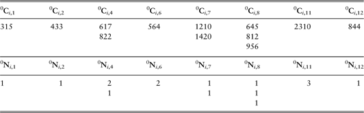
$--><$$>{\pre}^{0}{{C^{\Prime}}_{i,2,1}}\: = \:433,{\pre}^{0}{{C^{\Prime}}_{i,4,1}}\: = \:617,{\pre}^{0}{{C^{\Prime}}_{i,7,1}}\: = \:1420,{\pre}^{0}{{C^{\Prime}}_{i,8,1}}\: = \:645,{\pre}^{0}{{C^{\Prime}}_{i,11,1}}\: = \:2310,{\pre}^{0}{{C^{\Prime}}_{i,12,1}}\: = \:844.\eqno<$$><!--$

Table 1, after the introduction of the third trajectory becomes:

Table 1 Value of the vectors $)(--><$>{\pre}^{0}{{{\bf {{C}}}}_{i,{{k}_s}}}<$><$>{\pre}^{0}{{{\bf {{N}}}}_{i,{{k}_s}}}<$><!--$ after two steps

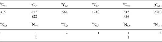
Greater clarification is offered in Table 2. After two trajectory constructions we had 8 different times in which a transition arrived. Times 1, 2 and 11 happened once, times 6 and 7 twice. The two extractions related to time 6 had the same cost whereas the two at time 7 had two different costs. At last times 4, 8 and 11 three times respectively with two, three and one type of cost. All this information can easily be read in the table.

Table 2 Value of the vectors $)(--><$>{\pre}^{0}{{{\bf {{C}}}}_{i,{{k}_s}}}<$><$>{\pre}^{0}{{{\bf {{N}}}}_{i,{{k}_s}}}<$><!--$ after three steps

The program for each starting state will construct 1,000,000 trajectories twice. If there are 40,000 claims at time 1 in the state 2 (OC) we will carry out 250 repetitions for the first construction and another 250 for the second after which the comparison of the results can be carried out.

The $)(--><$>{\pre}^{0}{{{\bf {{C}}}}_{i,{{k}_s}}}<$><$>{\pre}^{0}{{{\bf {{N}}}}_{i,{{k}_s}}}<$><!--$ are a couple of the basic vectors of our simulation.

Remark 11: We suppose the evaluation is to be carried out at the end of year 0. We know what happened at the end of the starting year, but we do not know what will happen at the end of the next 12 years. □

Remark 12: The program will construct ∀i, where i is not an absorbing state, the two tables ⁰C_i and ⁰N_i. that will be ordered in function of the year and for each year in increasing order of the cost. □

We could now evaluate the r.v. that we are looking for. The r.v. values will be given by all the different $)(--><$>{\pre}^{0}{{{\bf {{C}}}}_{i,{{k}_s}}}<$><$>{\pre}^{0}{{{\bf {{C}}}}_{i,{{k}_s}}}<$><$>{\pre}^{0}{{{\bf {{N}}}}_{i,{{k}_s}}}<$><$>{\pre}^{0}{{{\bf {{C}}}}_{i,{{k}_s}}}<$><$>{\pre}^{0}{{{\bf {{N}}}}_{i,{{k}_s}}}<$><!--$ .

Afterwards, the second simulation process will start. We will carry out the same number of trajectories as we carried out in the previous simulation process. If the values of the r.v. of the two simulations are the same and the probability distribution differs less than an ε, as was decided before the beginning of the simulation then our process will be stopped. Otherwise we will merge the two simulation processes considering the ⁰C_i,k obtained in both the processes and the corresponding occurrences ⁰N_i,k. This fact permits the computing of the new probability distribution. Now a new simulation process that will construct the double of the trajectories of the initial simulation process will be started.

The results obtained from the third simulation process will be compared to the simulation process obtained by the sum of the first two. If we obtain the conditions we want, then our process will be stopped, otherwise, we will merge the first three simulation processes and will start with the fourth simulation process that will be four times larger than the first process and we will continue this iterative process up to the point at which it converges.

In Figures 2.1 and 2.2 two trajectory examples are reported. The x-axis represents the time and the y-axis the states. The vertical lines with E and S at top represent, respectively, the states of the system and the possible costs of the claims. Now the trajectory given in Figure 2.1 will be described. The system starts at time 0 from the state j ₀. After the first two extractions the system will arrive at time 2 in the state j ₁. Now the cost of the claim due to the transition from j ₀ to j ₁ needs to be computed. We carry out another pseudo-random number extraction to obtain the cost γ ₁. This cost is discounted at time 0 and put in V ₀. Now with another two extractions the system arrives at time 3 in the state j ₂. Another extraction will give γ ₂, the cost of transition.

Figure 2.1 Example of trajectory that ends just at the end of horizon time

Figure 2.2 Example of trajectory with backward time 1 that ends before the end of horizon time

The discounted value at time 0 of this cost will be summed to V ₀ and so on. At the end of trajectory, when the time obtained is greater than T, the trajectory cost will be in V ₀.

This process will be repeated for each backward time and we will obtain $)(--><$>{\pre}^{h}{{{\bf {{C}}}}_{i,{{k}_s}}},\,{\pre}^{h}{{{\bf {{N}}}}_{i,{{k}_s}}}<$><!--$ , h = 0,1,…,T. In Figure 2.1, T = 7. Figure 2.2 shows the case in which a trajectory begins at time 1 because of the recurrence backward time 1 and ends because of a time extraction that surpasses the horizon time T.

6.2 Example of the merging process

We suppose that we have three different costs for each year and that the first simulation is stopped after the construction of 100 trajectories and that we start with a recurrence backward time 3. The results obtained in the first simulation are reported in Table 3.1.

Table 3.1 Value of the vectors $)(--><$>{\pre}^{3}{{{\bf {{C}}}}_{i,{{k}_s}}}<$><$>{\pre}^{3}{{{\bf {{N}}}}_{i,{{k}_s}}}<$><!--$ resulting from the first 100 trajectory simulations

In Table 3.2 the results of the second 100 trajectories are given. The two results are different so we merge the two results and we obtain Table 3.3. We suppose that the subsequent 200 simulations gave approximately the same results and we stop the simulation process.

Table 3.2 Value of the vectors $)(--><$>{\pre}^{3}{{{\bf {{C}}}}_{i,{{k}_s}}}<$><$>{\pre}^{3}{{{\bf {{N}}}}_{i,{{k}_s}}}<$><!--$ resulting from the second 100 trajectory simulations

Table 3.3 Value of the vectors $)(--><$>{\pre}^{3}{{{\bf {{C}}}}_{i,{{k}_s}}}<$><$>{\pre}^{3}{{{\bf {{N}}}}_{i,{{k}_s}}}<$><!--$ after the merging (200 trajectory simulations)

– At this point we merge the column of Table 3.3 and we obtain the results reported in Table 4. Dividing by 1488, which is the total number of occurrences we can find the probability distribution corresponding to the occurrences of Table 4. This result is reported in Table 5. If we pose that i = IBNR then Table 5 represents the r.v. of the single values of the different claim costs that are reported after three years of backward recurrence time. In Table 6 the corresponding r.v. of the possible total costs is given. Each total cost is obtained multiplying the single value of each cost by its recurrence (for the aim of simplicity we did not consider the repetitions). In Table 7 the increasing total cost (i.t.c) and the related increasing d.f. are reported summing the elements of the value and probability columns given in Table 6. In Figure 3 the graphs of the i.t.c. and of the i.d.f. are shown. The Capital at Risk (CaR) corresponding to 99.5% SCR (Solvency Capital Requirement) and 75% MCR (Minimum Capital Requirement) as supposed in Janssen & Manca (Reference Janssen and Manca2009) are also reported in the figure. The example explains how to get the results for the state i and the backward time 3.
– Fixing the state and the time and merging on the backward times it is possible to obtain the r.v. of the costs for the fixed year and the given state.
– It is possible to fix the year and the backward time and in this way we can merge with respect to the states having the r.v. of the costs for the given year and backward time as results.

Figure 3 Graphs of Table 7 with SCR and MCR

Table 4 Merging of all the elements of the Table 3.3. done on the columns (state i and backward 3)

Table 5 r.v. of all possible unitary costs, the distribution probability is obtained dividing each occurrence by the total number of occurrences

Table 6 r.v. of costs of each value obtained multiplying the values for the corresponding occurrences

Table 7 Increasing total cost and its distribution function

Now we suppose that we have constructed the two matrices for all the backward time and the states; i.e. we have constructed

$--><$$> {\pre}^{b}{{{\bf {{C}}}}_{i,k}},{\pre}^{b}{{{\bf {{N}}}}_{i,k}},\,k\: = \:b\: + \:1, \ldots, T,\,\,\,\forall b\: \in \:\left\{ {0,1, \ldots, T{\rm{ - }}1} \right\},\forall i\: \in \:E \eqno<$$><!--$

– If we fix the state and the backward time and we merge with respect to the years of the horizon time we obtain the two vectors that represent the possible unitary costs and their occurrences (Table 4 is an example of these two vectors);
– If we divide the vector of occurrences by the total number of occurrences we obtain the r.v. of the possible unitary costs given the backward time and the state (Table 5 is an example of this r.v.);
– If we multiply the single costs for their occurrences (the second and third vector of Table 4) and we associate the elements of the probability distribution contained in the third column of Table 5 to the results, we obtain the r.v of the total cost of each single value (Table 6 is an example of this r.v.).
– If we sum the elements of the probability column we obtain the i.d.f. of the total costs of each single value
– If we sum the elements of total cost column of each single value we obtain the related i.t.c. and i.d.f. (Table 7 is an example of this last result).
– If we fix the state and we apply the merging process on the backward time, for each state we will obtain two vectors for each state that will represent the possible unitary costs and their occurrences for the fixed state. (We can also fix the backward time and apply the merging process to the states thereby obtaining, for each backward time two vectors that will represent the r.v. that gives the unitary costs for each backward recurrence time and their occurrences):
– If we divide each element of the vector of occurrences by the total number of occurrences and we associate this probability distribution to the vector of single unitary costs we obtain the r.v. of the possible unitary costs given the fixed state;
– if we multiply each single cost by its occurrences and we associate at these results to the vector of the probability distribution we will obtain the r.v. that gives the total cost for the fixed state;
– after this process, we have 6 different couples of vectors, one for each state, that we then consider. In each vector there are all the possible unitary costs for each considered state and the related unitary costs. Now we can merge these 6 couple of vectors and we will obtain two vectors that will represent all the possible unitary costs that the company could have in the studied horizon and their occurrences:
– If we divide each element of the vector of occurrences by the total number of the related occurrences and we associate this probability distribution to the vector of all possible single unitary costs we will obtain the r.v. of all the possible unitary costs;
– if we multiply each single cost by its occurrences and we associate the vector of the probability distribution to these results, we will obtain the r.v. that gives the total costs for the considered horizon time.

This last variable is the r.v of the claim reserving for the studied insurance company.

Once we have this r.v. we can compute any moment. So we can obtain the mean total cost of the claims in the considered horizon, the related standard deviation, the skewness and the kurtosis. Clearly it is possible to compute any quantile so any fixed value of the VaR.

Furthermore, the model gives a lot of information. For example if we want to know the claim costs for each year of the considered horizon time it can be obtained applying the merging process to the backward time and to the states which allows us to obtain the r.v. of the claim costs for each year. We can obtain the mean cost of claims, the VaR, the standard deviation and so on. We could obtain the r.v. for each year of the horizon time and each state merging with respect to the backward recurrence time. We could also obtain the r.v. for each year and for each backward recurrence time beginning the merging process on the states.

It is evident that by means of this model it is possible to obtain in a natural way results that the other claim reserving models do not give. By means of these results the insurance company could decide its industrial strategies or find its weaknesses.

Once again we would like to state that the IBNyR and the IBNeR claims will be evaluated in a natural way and, from the point of view of semi-Markov process, without increasing the quantity of data that are necessary to the process to be applied, as clearly explained in D'Amico et al. (Reference D'Amico, Guillen and Manca2009).

Remark 13: We use a fixed risk free interest rate r but we could use an interest rate structure in the same way and also a stochastic interest rate structure without any problems. Clearly with a stochastic interest rate structure the simulation number of trajectories should be increased. □

7. An example of claims reserve distribution construction

7.1. The Program Inputs

To apply the model described in the two previous sections it is necessary to have the history of each claim: when the claim incurred, when it was reported, when it was partially paid, what the cost of this payment was and so on. Each insurance company has these data although it is not always easy to obtain them. We are not able to have access to raw data of the claim stage evolution so we were not able to construct the P and F matrices as they should be. We could only obtain 4 years (2005–2008) of a table in which the claim history of one of the most important Italian insurance companies is summarised. Each table shows all the not yet settled claims of the past years that are in the company portfolio at the beginning of the year, together with the information about the time elapsed since the claims. The reported claims in the year were also provided. In this way, it was possible to have an idea of the IBNyR claims but not of their evolution. We could also have computed the mean claims costs for each different case, but we knew nothing about the claims cost distributions. The situation at the end of the year is also given in the tables. For this reason it is possible to have an idea of claims evolution and the transitions among the states.

To construct an example we started with this information and we constructed the transition matrix P. The transition matrix was constructed in the correct way for a Markov process because we knew the initial number of claims and which of them had changed their stage within the year. Clearly, the transition matrix of the Markov chain is different by the transition matrix embedded in the semi-Markov process. In order to understand this better, we report the graph connected to the matrix in Figure 4 and the claims stage definition already given in the introductory section.

1. IBNyR claims (IBNR),
2. Open Claims (OC),
3. Partially Paid claims (PP),
4. Reopened Claims (RC),
5. Without Payment closed claims (CWP),
6. Closed Claims with payment (PCC),

Figure 4 The Markov chain graph of the claims stages

The stages of the claims were chosen in function of the subdivision given in the tables. The transitions were also constructed in function of the data that we got from the tables.

From the data, it results that the PCC is an absorbing state. We cut the possibility of transitions that go from state 6 to the other states, but it is very simple to introduce it into the model. PCC being an absorbing state we considered 5 starting states.

The F values were also obtained from our data attempting to use our information, in this case not too many, in the best way. Regarding the r.v. claims costs we had the mean from data, aiming to simplify we gave four other values; two smaller and two greater than the mean. After, we construct the related probability distributions without any data but attempting to be rational.

We worked on a time interval of 13 years. We supposed that inflation was fixed at 1% and that the risk-free interest rate was 2%.

The model takes into account the evolution of backward times for each year of the studied horizon time in a natural way. However, for each year and for each starting state it is necessary to know the number of related claims. More precisely, it is necessary to give as input the number of the claims that are in the states 2, 3, 4 and 5 at time 0 (state 1 has at least 1 year of backward and state 6 is supposed absorbing and it makes no sense to start from it) and we had these data. Furthermore, for each starting state (state from 1 to 5) we should know how many claims have 1, 2,…,T backward times (the time in which they entered in the state and did not move from it). For IBNyR stage we had this information but not for the other states. Taking into account the IBNyR stage data and the ratio among the claim numbers of IBNyR and of the claim numbers of the other states we also constructed the number of claims for each backward time and for the 4 other starting states. These inputs are reported in Table 8.

Table 8 Supposed claims number for each state and backward time

We have, starting from the year 1, 61 different kinds of situations and we constructed the same initial trajectory number for each of them.

For example if we wished to simulate 1,000,000 trajectories for each kind of claim we divided 1,000,000 by the number of starting claims and we calculated how many trajectory repetitions we needed to carry out for the case being studied.

For example we have, at year 0, 14853 claims in the state PP. The number of repetition to obtain at least 1,000,000 trajectories is given by:

$--><$$>\left\lceil {\frac{{1000000}}{{14853}}} \right\rceil \: = \:68\eqno<$$><!--$

In the end we divided the results by the number of trajectory repetitions (in our example 68) and we could get the results for the case being studied and having the same reliability in all the cases because we construct the same initial number of trajectories for all the cases.

Remark 14: We started with 1,000,000 trajectories for each case because we believe that in order to have meaningful results for a complex phenomenon by means of Monte Carlo method it is necessary to start with this number of trajectories. It is also possible to work with a smaller number but if the Monte Carlo is performed with the iterative process described before, we think that the convergence will be obtained with about the starting number of trajectories as ours. □

In Figures 5 and 6, the embedded Markov Chain and the waiting time distribution functions with starting states 1 (IBNR) and 2 (OC) and arriving states 2, 3 (PP), 5 (CWP), 6 (PCC) are reported.

Figure 5 Markov Chain embedded in the SMP

Figure 6 Waiting time d.f. with starting states IBNR and OC

7.2. The Model Results

The model presented solves firstly, the DTHSMP with backward times and gives a lot of information on the evolution of the claim stages. For example, it gives the probability that a claim that has 3 years of backward time (the accident occurred 3 years before being reported), starting from the IBNyR state will be paid after 4 years. We decided not to discuss these aspects of our study preferring, instead, to concentrate on the reconstruction of the claim reserve distribution.

The best way to describe how the model works is to briefly describe the algorithm and then to explain the results that were obtained in the most important steps.

7.2.1. The algorithm description

We work in a discrete time environment and the year is the unit. This is normal because the insurance companies usually work with this time scale.

First step: INPUTS.

Different inputs of the program:

– the state number,
– the time horizon length,
– the chosen approximation for Monte Carlo application. i.e. for each starting state and time two simulations with the same number of trajectories will be done, each of them will construct a random variable. If the values of the two r.v. are equal and the related probability functions differs (euclidean distance between two vectors) less than the chosen approximation ε, then we stop the simulation process of the examined case.
– the maximum number of values that each evaluated r.v. can assume (it might be possible that an r.v. can assume too many different values and it could give the program problems. This input establishes the maximum number of values that the r.v. can assume),
– the state number from which it makes sense to start (number of non-absorbing states),
– the rate of interest and of inflation,
– the embedded Markov chain P,
– the matrix of waiting time d.f. F,
– the claim number for each starting state and backward time (Table 8)
– the r.v. of the costs for each time and transition.

Second step: DTHSMP with backward recurrence time evolution equation solution.

The program gives the first results that are:

– the solution of the evolution equation (3.4) the probabilities of which are defined in (3.1) (for more details on this step see Corradi et al., Reference Corradi, Janssen and Manca2004 and Stenberg et al., Reference Stenberg, Manca and Silvestrov2006).
– the probabilities that the next transition will be in a given state given that up to time t there were no transitions. These probabilities are defined in this way:

$--><$$> {{\varphi }_{ij}}(t)\: = \:{\rm{P}}\left[ {{{J}_{n\: + \:1}}\: = \:j|{{J}_n}\: = \:i,\,{{T}_{n\: + \:1}}{\rm{ - }}{{T}_n}\: \gt \:t\,} \right] \eqno<$$><!--$

Both these pieces of information could be useful for insurance company managers. In this step the H_i(l;t) and the b_ij(l;t) that will be used for the simulations are also computed.

Third step: Construction of the basic vectors with 0,1,…,T-1 backward recurrence time

For each year k_s and starting state i and for each backward time h = 0,1,…,T−1, 2 vectors are constructed: the $)(--><$>{\pre}^{h}{{{\bf {{C}}}}_{i,{{k}_s}}} <$><$>{\pre}^{h}{{{\bf {{N}}}}_{i,{{k}_s}}}<$><!--$ (see Tables 1, 2, 3.1, 3.2, 3.3).

– each element of the $)(--><$>{\pre}^{h}{{{\bf {{N}}}}_{i,{{k}_s}}} <$><!--$ contains the number of times in which a cost is obtained during all the foregone Monte Carlo simulations including the repetitions,
– each element of the $)(--><$>{\pre}^{h}{{{\bf {{C}}}}_{i,{{k}_s}}} <$><!--$ contains a different cost. Different costs are in different vector positions,
– the $)(--><$>{\pre}^{h}{{{\bf {{C}}}}_{i,{{k}_s}}} <$><!--$ is ordered in increasing order.

This is the most important step of the algorithm and the iteration begins here in order to decide when the simulation can be stopped.

This step was explained in the previous section and we would only add that, at the end of this step, we will divide the vectors $)(--><$>{\pre}^{h}{{{\bf {{N}}}}_{i,{{k}_s}}} <$><$>{\pre}^{h}{\bf {{N}}}_{{i,{{k}_s}}}^{'} <$><$>{\pre}^{h}{\bf {{N}}}_{{i,{{k}_s}}}^{'} <$><$>{\pre}^{h}{{{\bf {{C}}}}_{i,{{k}_s}}}<$><$>{\pre}^{h}{\bf {{N}}}_{{i,{{k}_s}}}^{'} <$><$>{\pre}^{h}{\bf {{C}}}_{{i,{{k}_s}}}^{'} <$><$>{\pre}^{h}{\bf {{N}}}_{{i,{{k}_s}}}^{'} <$><$>{\pre}^{h}\hskip 7pt{\bf {{\vskip -5pt\hat\hskip -7pt} {N}}}}_{{i,{{k}_s}}}^{{}} <$><$>{\pre}^{h}{\bf {{C}}}_{{i,{{k}_s}}}^{'} <$><!--$ values.

Fourth step: Merging of the basic vectors in function of time

Now the vectors obtained in the third step are merged with regards to the time. We merge all the vectors that have the same starting state and backward time. The merging is done on the values of claim costs that are in increasing order. If there are two equal values the corresponding occurrences are summed. The first year values will be merged with the ones of the second year. The obtained vector will be merged with the third year values. The obtained vector will be merged with the fourth year values and so on. At the end of this process we will have two vectors for each starting state and for each backward time. In one vector there will be all the different values of the claim costs related to the starting state and the considered backward time. In the other vector their occurrences. At the end of this step we will obtain ^hC_i and $)(--><$>{\pre}^{h}{\bf {{N}}}_{i}^{'} <$><$>{\pre}^{h}{\bf {{N}}}_{i}^{'} <$><$>{\pre}^{h}{\bf {{C}}}_{i}^{'} <$><$>{\pre}^{h}\hskip 7pt{\bf {{\vskip -5pt\hat\hskip -7pt}{N}}}}_{i}^{'} <$><!--$ will be calculated. They will contain, respectively, the total cost for each different value and the related probability function.

In particular if we look at the two vectors $)(--><$>{\pre}^{h}{\bf {{C}}}_{{IBNR}}^{'} <$><$>{\pre}^{h}\hskip 7pt{\bf {{\vskip -5pt\hat\hskip -7pt}{N}}}}_{{IBNR}}^{'} <$><!--$ we have the r.v. of the incurred but not reported claims that are reported after h years.

Fifth step: Merging of the vectors in function of the states

This is similar to the fourth step. After the merging on times, the merging is done on the states. The final result will give ^hC and ^hN′. In this case the ^hC′ and $)(--><$>{\pre}^{h}\hskip 7pt{\bf {{\vskip -5pt\hat\hskip -7pt}{N}}}}}^'} <$><!--$ will be also calculated.

Sixth step: Results in function of the backward time

Now we have two vectors for each backward recurrence time. We will carry out the last merging process on the couple of vectors ^hC and ^hN′ so after this last process we will obtain the two vectors C and N′ that respectively contain all the possible values of the unitary costs of claims and the related occurrences. From these values we will obtain C′ and $)(--><$>{{{\bf {{\hat{N}}}}}^'} <$><!--$ where:

C′ contains the total cost related at each unitary value. It will be obtained multiplying the elements of C by the corresponding elements of N′

$)(--><$>{{\hskip 7pt{\bf {{\vskip -5pt\hat\hskip -7pt}{N}}}}}^'} <$><!--$ contains the probability mass distribution related to the elements of C′.

This couple of vector is the r.v. of the claim reserve of the studied car-insurance company. And it will be possible to compute any moment of this and any quantile and so any VaR value.

Remark 15: It is possible to arrive to the vectors C′ and $)(--><$>{{{\bf \hskip 7pt{\bf {{\vskip -5pt\hat\hskip -7pt}{N}}}}}^'} <$><$>{\bf {{C}}}_{t}^{'} <$><$>{\bf \hskip 7pt{\bf {{\vskip -4pt\hat\hskip -7pt}{N}}}}_{t}^{'} <$><!--$ , {t = 1,…,T} that will represent the r.v. of the costs that the insurance company has to pay for each year of the studied horizon. In this case the couple of vectors will represent the r.v of the costs for each starting state.

Merging these couples and storing the results for each year of the time horizon will give the r.v. of the total costs that the insurance company will have to pay up to a given year for the claims that have been incurred but have not yet been settled.

Finally, merging before on the horizon time and after on backward recurrence times the costs that depend on the starting state $)(--><$>{\bf {{C}}}_{i}^{'} <$><$>{\bf \hskip 7pt{\bf {{\vskip -5pt\hat\hskip -7pt}{N}}}}_{i}{\vskip -12pt'} <$><!--$ , i ∈ E will be obtained. □

7.2.2. The claim reserving results

The presented model gives a lot of information on the claim reserve problem.

– Information obtained by the DTSMP with backward recurrence time evolution equation:

^bφ_ij(l;t): probability of being at time t in the state j given that at time 0 the system was in the state i and that it arrived in this state l time before.

For example, ^bφ _1,6(3;5) gives the probability that an IBNyR claim which occurred 3 years before and which was reported today will be closed with a payment within 5 years. In the IBNeR case ^bφ _2,5(2;7) gives the probability that at time 0 an open claim that arrived in this state 2 years before will be closed without payments within 7 years.

φ_ij(t): probability of going into the state j with the next transition given that the system does not move from the state i up to the time t. For example, φ _3,6(8) is the probability that a partially paid claim without transition up to the year 8 will be closed with payment.

b_ij(l;t): probability of having a transition from state i to the state j exactly at time t given that at time 0 the system was in the state i and that it arrived in this state l time before, b _1,3(4;6) is the probability that a claim which occurred 4 years before being reported today will be partially paid exactly after another 6 years.

Other information could be obtained by means of the evolution equation parameters but we think that the presented cases are the most important.

– Information given by the simulation model:

The simulation model gives many and important results for the study of the claim reserve problem. We know the situation at time 0.

1. The vectors $)(--><$>{\pre}^{h}{{{\bf {{C}}}}_{i,{{k}_s}}} <$><$>{\pre}^{h}{\bf {{N}}}_{{i,{{k}_s}}}^{'} <$><$>{\pre}^{{\rm{h}}}{\bf {{N}}}_{{i,{{k}_s}}}^{'} <$><$>{\pre}^{h}{\bf \hskip 7pt{\bf {{\vskip -5pt\hat\hskip -7pt}{N}}}}_{{i,{{k}_s}}}^{'} <$><$>{\pre}^{h}{\bf {{C}}}_{{i,{{k}_s}}}^{'} <$><$>{\pre}^{h}{\bf \hskip 7pt{\bf {{\vskip -5pt\hat\hskip -7pt}{N}}}}_{{i,{{k}_s}}}^{'} <$><$>{\pre}^{h}{{{\bf {{C}}}}_{i,{{k}_s}}}<$><$>{\pre}^{h}{\bf \hskip 7pt{\bf {{\vskip -5pt\hat\hskip -7pt}{N}}}}_{{i,{{k}_s}}}^{'} <$><$>{\pre}^{h}{\bf {{C}}}_{{i,{{k}_s}}}^{'} <$><$>{\pre}^{h}{\bf {{N}}}_{{i,{{k}_s}}}^{'} <$><$>{\pre}^{h}{{{\tilde{\bf C}}}}_{{i,{{k}_s}}}^{'} <$><!--$ that represents another evaluation of the total cost r.v. values. It should be noted that having reconstructed the r.v. we could, also at this level, reconstruct at any moment, any variability measure and any risk evaluation.
2. The vectors $)(--><$>{\pre}^{h}{{{\bf {{C}}}}_t},\,{\pre}^{h}{\bf {{N}}}_{t}^{'}, \,\,\,\,h,t\: = \:\{ 0,1, \ldots, T\} <$><$>{\pre}^{h}{{{\bf {{\hskip 7pt{\bf {{\vskip -5pt\hat\hskip -7pt}{N}}}}}_t} <$><$>{\pre}^{0}{\bf {{N}}}_{t}^{'}, \,t\: = \:1, \ldots, T<$><$>{\pre}^{0}{\bf {{C}}}_{t}^{'}, \,t\: = \:1, \ldots, T<$><$>{\pre}^{0}{\bf {{C}}}_{1}^{'} <$><$>{\pre}^{0}{{{\bf \hskip 7pt{\bf {{\vskip -5pt\hat\hskip -7pt}{N}}}}}_1}<$><$>{\pre}^{0}{\bf {{C}}}_{1}^{'} <$><$>{\pre}^{0}{{{{{\bar{\bar{\bf C}}}}}}}_{1}^{'} <$><$>{\pre}^{h}{{{\bf {{C}}}}_t},\,{\pre}^{h}{\bf {{N}}}_{t}^{'}, \,\,\,\,h,t\: = \:\{ 0,1, \ldots, T\} <$><!--$ , the IBNyR and the IBNeR with backward time are evaluated naturally.
3. ⁰C and ⁰N′ contain respectively all the different unitary costs that were made necessary by the claims with no backward recurrence times and their occurrences. As explained in the previous cases from ⁰N′ we can compute $)(--><$>{\pre}^{{{\pre}^{0}}}{{{\bf \hskip 7pt{\bf {{\vskip -5pt\hat\hskip -7pt}{N}}}}}^'} <$><$>{\pre}^{0}{\bf \hskip 7pt{\bf {{\vskip -5pt\hat\hskip -7pt}{N}}}}<$><$>{\pre}^{0}{{{{{\bar{\bf C}}}}}^'} <$><$>{\pre}^{0}{{{{{\bar{\bar{\bf C}}}}}}^'} <$><$>{\pre}^{h}{{{{{\bar{\bar{\bf C}}}}}}^'}, \,\,\,\forall h = 1, \ldots, T<$><!--$ too.
4. As observed before we will obtain the C and N′. The first vector contains all the unitary costs that were encountered during the simulation steps. The related occurrences are in the second vector. We can calculate the C′ by multiplying the elements of C by the corresponding elements of N′. $)(--><$>{{{\bf \hskip 7pt{\bf {{\vskip -5pt\hat\hskip -7pt}{N}}}}}^'} <$><!--$ will be obtained by dividing each of its elements by their sum. In this way we obtain another r.v. in which their values are the total cost for each possible unitary cost and the probability distribution of the total costs. We have constructed the claim reserve r.v. We can construct any moment of these r.v., any variability index and any risk measure.

7.2.3. An “almost” real life example

As already mentioned, we do not have the raw data necessary to construct the right input for DTHSMP, we used the data that summarise 4 years (2005–2008) of claims of one of the most important Italian insurance companies and were already described in section 7.1. By means of these data we could give an evaluation of the input that is necessary for our model; hence “almost” in the title of this subsection. We believe, however, that, with this example, we could show the possible results that can be obtained by our model. In this section we give the results of the model obtained by the data given in section 7.1.

Firstly, two matrices of the evolution equation solution are reported in Figures 7.1 and 7.2. The matrix elements show that with different backward times different solutions are obtained.

Figure 7.1 Evolution equation solution at time 5 with backward time 1

Figure 7.2 Evolution equation solution at time 5 with backward time 5

Remark 16: The results are very different. For example in the IBNyR case, if we start with a backward time 1 then, most of them, will be reported within the next year. On the other hand, if we start with backward equal to 5, most of the not yet reported claims will remain in the IBNyR in the next year. □

In Figure 8.1 the total costs that come from Open Claim stage and the related d.f. are reported. This graph shows the costs that the insurance company will pay considering all the claims that entered into the system in the stage of Open Claim and the related d.f. Figure 8.2 reports the same but in the case of IBNyR stage.

Figure 8.1 Total costs that come from the open claim starting stage

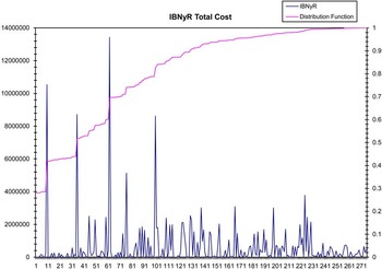
Figure 8.2 Total costs that come from the IBNyR claim starting stage

Figures 9.1 and 9.2 show the total costs that come from all the claims that were reported for year 1 and year 5 respectively. The related d.f. are also shown in the graph.

Figure 9.1 Total costs that come from the reported claims in the year 1

Figure 9.2 Total costs that come from the reported claims in the year 5 with the related D.F.

Figure 10 reports all the 338 different costs that were found during the simulation. The costs are in increasing order. The pink graph gives the value of the cost and the blue graph the number of claims corresponding to the unitary costs. It should be mentioned that the most frequent case is the case of no claim reimbursement; more than 1/3 of the cases.

Figure 10 Total numbers and unitary costs of accidents in the 12 years

The blue graph of Figure 11 is the same as Figure 10 while the pink graph shows the d.f. of different costs.

Figure 11 Unitary costs with the related distribution function

Finally, Figure 12 shows the total cost and the related d.f. that is clearly the same as the previous figure.

Figure 12 Total cost and the related distribution function with SCR and MCR calculation

In the figure the SCR and the MCR are outlined. The MCR is at a very low level but the fact that more than 1/3 of the claims will be closed without any payment should be taken into account.

8. Conclusions

In this paper we have presented a totally new approach to the solution of the claim reserving problem while taking into account the SCR and the MCR as defined by the new Solvency II rules.

The problem is solved following the evolution of the claim stages. It is supposed that this evolution works under a discrete time semi-Markov hypotheses with initial backward recurrence time. The algorithm used to get the solution and which permits the availability of all the possible probability distributions derives from a Monte Carlo simulation model.

We do not think that this model is a “panacea” for the claim reserving model but we feel the paper contributes significantly to the considerable scientific debate that is taking place at the moment.

We should mention that the introduction of backward time permits the taking into account the IBNyR claims in a natural way. Indeed the initial backward time is attached to a stochastic process which permits the consideration of the events that happened before the time in which the observed system begins to be followed.

We could not get the data that are necessary in order to apply in a more satisfactory way a semi-Markov process. For this reason some of the real life aspects could be developed better by using the data that are necessary for the application of SMP.

In our opinion, in order to understand the full potential of a new model it is important to have the correct data. In the same time we think that this paper gives an idea of the potential of our model.

In the near future we hope to obtain the real data that could serve as the correct input for our semi-Markov model.

If we succeed in this we will apply our model and we would like to compare our results with the results that can be obtained from the other models that are used for the reconstruction of the claim reserve probability distribution.

Acknowledgements

The authors are grateful to colleagues and friends Guglielmo D'Amico and Dmitrii Silvestrov for the discussions on the SMP simulation model. The authors are also grateful to the comments and the suggestions of anonymous referees and of the editor of AAS that improved substantially this paper.

References

Ashe, F.R. (1986). An essay at measuring the variance of estimates of outstanding claim payments. ASTIN Bulletin, 16, 99–113.Google Scholar

Australian Prudential Regulation Authority (1999). A new statutory solvency standard for general insurers.Google Scholar

Balcer, Y., Sahin, I. (1986). Pension accumulation as a semi-Markov reward process, with applications to pension reform. In J. Janssen Semi-Markov models. Plenum N.Y.Google Scholar

Barbu, V., Boussemart, M., Limnios, N. (2004). Discrete-time semi-Markov model for reliability and survival analysis. Communications in Statistics: Theory and Methods, 33, 2833–2868.CrossRef Google Scholar

Biffi, E., Janssen, J., Manca, R. (2007). Un modello Monte Carlo semi-Markoviano utile alla misura della riserva sinistri. Proceedings of the VIII congresso Nazionale degli Attuari. Trieste.Google Scholar

Biffi, E., D'Amico, G., Di Biase, G., Janssen, J., Manca, R., Silvestrov, D. (2008a). Monte Carlo semi-Markov methods for credit risk migration models and Basel II rules II. Zhurnal Obchyslyuval'no Ta Prykladno I Matematyky, 96, 59–86.Google Scholar

Biffi, E., D'Amico, G., Di Biase, G., Janssen, J., Manca, R., Silvestrov, D. (2008b). Monte-Carlo semi-Markov methods for credit risk migration models and Base II rules. I. Zhurnal Obchyslyuval'no Ta Prykladno I Matematyky, 96, 28–58.Google Scholar

Bjökwall, S., Hössjer, O., Ohlsson, E. (2009). Non-parametric and parametric bootstrap techniques for age-to-age development factor methods in stochastic claim reserving. Scandinavian Actuarial Journal, 306–331.Google Scholar

Bornhuetter, R.L., Ferguson, R.E. (1972). The actuary and IBNR. Proceedings CAS, LIX, 181–195.Google Scholar

Christofides, S. (1990). Regression models based on logincremental Payments. In Claims Reserving Manual, 2, Institute of Actuaries, London.Google Scholar

Corradi, G., Janssen, J., Manca, R. (2004). Numerical treatment of homogeneous semi-Markov processes in transient case. Methodology and Computing in Applied Probability, 6, 233–246.Google Scholar

D'Amico, G., Guillen, M., Manca, R. (2009). Full backward non-homogeneous semi-Markov processes for disability insurance models: a Catalunya real data application. Insurance: Mathematics and Economics, 45, 173–179.Google Scholar

De Alba, E. (2002). Bayesian estimation of outstanding claim reserves. North American Actuarial Journal, 6, 1–20.Google Scholar

De Dominicis, R., Manca, R. (1984a). Numerical treatment of homogeneous semi-markov processes. Proceedings of the VI meeting “Computer at University”. Dubrovnik, (1984). Available on line at http://dimadefa.eco.uniroma1.it/manca/Numerical_treatment.pdf.Google Scholar

De Dominicis, R., Manca, R. (1984b). An algorithmic approach to non-homogeneous semi-Markov processes. Communications in Statistics Simulation and Computation.Google Scholar

De Medici, G., Janssen, J., Manca, R. (1995). Financial operation evaluation: a semi-Markov approach. Proc. V AFIR Symposium. Brussels.Google Scholar

England, P.D. (2002). Addendum to “Analytic and bootstrap estimates of prediction errors in claims reserving”. Insurance: Mathematics and Economics, 31, 461–466.Google Scholar

England, P.D., Verrall, R.J. (1999). Analytic and bootstrap estimates of prediction errors in claims reserving. Insurance: Mathematics and Economics, 25, 281–293.Google Scholar

England, P.D., Verrall, R.J. (2002). Stochastic claims reserving in general insurance. British Actuarial Journal, 8, 443–510.Google Scholar

England, P.D., Verrall, R.J. (2005). Incorporating expert opinion into a stochastic model for the chain-ladder technique. Insurance: Mathematics and Economics, 37, 355–370.Google Scholar

England, P.D., Verrall, R.J. (2006). Predictive distribution of outstanding liabilities in general insurance. Annals of Actuarial Science, 1, 221–270.CrossRef Google Scholar

Faculty and Institute of Actuaries (1997). Claims Reserving Manual. 2 volumes.Google Scholar

Gigante, P., Sigalotti, L. (2005). Model risk in claims reserving with generalized linear models. Giornale dell'Istituto Italiano degli Attuari, LXVIII, 55–87.Google Scholar

Haastrup, S., Arias, E. (1996). Claims reserving in continuous time a non parametric Bayesian approach. ASTIN Bulletin, 26, 139–164.CrossRef Google Scholar

Haberman, S., Pitacco, E. (1999). Actuarial models for disability insurance. Chapman & Hall.Google Scholar

Hesselager, O. (1994). A Markov model for loss reserving. ASTIN Bulletin, 24, 183–193.CrossRef Google Scholar

Hoem, J.M. (1972). Inhomogeneous semi-Markov processes, select actuarial tables, and duration-dependence in demography. in T.N.E. Greville, Population, Dynamics. Academic Press, 251–296.Google Scholar

Janssen, J. (1966). Application des processus semi-markoviens à un probléme d'invalidité. Bulletin de l'Association Royale des Actuaries Belges, 63, 35–52.Google Scholar

Janssen, J., De Dominicis, R. (1984). Finite non-homogeneous semi-Markov processes. Insurance: Mathematics and Economics, 3, 157–165.Google Scholar

Janssen, J., Manca, R. (1997). A realistic non-homogeneous stochastic pension funds model on scenario basis. Scandinavian Actuarial Journal, 113–137.Google Scholar

Janssen, J., Manca, R. (2006). Applied semi-Markov Processes. Springer Verlag, New York.Google Scholar

Janssen, J., Manca, R. (2007). Semi-Markov risk models for Finance, Insurance and Reliability. Springer, New York, NY, USA, 2007.Google Scholar

Janssen, J., Manca, R. (2009). Outils de construction de modèles internes pour les assurances et les banques. Hermes and Lavoisier, Paris.Google Scholar

Kirschner, G.S., Kerley, C., Isaacs, B. (2002). Two approaches to calculating correlated reserve indications across multiple lines of business. CAS Forum (Fall), 211–246.Google Scholar

Levy, P. (1954). Processus semi-Markoviens. Proc. of International Congress of Mathematics, Amsterdam.Google Scholar

Limnios, N., Oprişan, G. (2001). Semi-Markov Processes and Reliability. Birkhauser, Boston.CrossRef Google Scholar

Liu, H., Verrall, R.J. (2009). Predictive distributions for reserves which separate true IBNR and IBNeR Claims. ASTIN Bulletin, 39, 35–60.CrossRef Google Scholar

Mack, T. (1993). Distribution-free calculation of the standard error of chain-ladder reserve estimates. ASTIN Bulletin, 23, 213–225.Google Scholar

Mack, T. (1994). Which stochastic model is underlying the chain ladder model? Insurance: Mathematics and Economics, 15, 133–138.Google Scholar

Mack, T. (1999). The standard error of chain ladder reserve estimates recursive calculation and inclusion of a tail factor. ASTIN Bulletin, 29, 361–366.Google Scholar

Mack, T. (2008). The prediction error of Bornhuetter/Ferguson. ASTIN Bulletin, 38, 87–103.CrossRef Google Scholar

Merz, M., Wüthrich, M.V. (2006). A credibility approach to the Munich chain-ladder method. Blätter DGVFM, XXVII, 619–628.CrossRef Google Scholar

Merz, M., Wüthrich, M.V. (2007). Prediction error of the expected claims development result in the chain ladder method. Schweiz. Aktuarver. Mitt., 5, 117–137.Google Scholar

Norberg, R. (1993). Prediction of outstanding liabilities in non-life insurance. Astin Bulletin, 23(1), 95–115.CrossRef Google Scholar

Norberg, R. (1999). Prediction of outstanding claims: Model variations and extensions. Astin Bulletin, 29(1), 5–25.CrossRef Google Scholar

Ntzoufras, I., Dellaportas, P. (2002). Bayesian modelling of outstanding liabilities incorporating claim count uncertainty. North American Actuarial Journal, 6, 113–128.CrossRef Google Scholar

Peters, G.W., Shevchenko, P.V., Wüthrich, M.V. (2009). Model uncertainty in claim reserving within Tweedie's compound Poisson models. Astin Bulletin, 39, 1–33.Google Scholar

Pinheiro, P.J.R., Andrade e Silva, J.M., de Lourdes Ceneno, M. (2003). Bootstrap methodology in claim reserving. The Journal of Risk and Insurance, 70, 701–714.Google Scholar

Quarg, G., Mack, T. (2004). Munich chain ladder. Blätter DGVFM, XXVI, 597–630.CrossRef Google Scholar

Renshaw, A.E. (1989). Chain ladder and interactive modelling (claim reserving and GLIM). Journal of the Institute of Actuaries, 116, 559–587.Google Scholar

Schmidt, K.D. (2010). A Bibliography on Loss Reserving. Available online at the address http://www.math.tu-dresden.de/sto/schmidt/dsvm/reserve.pdf.Google Scholar

Schnieper, R. (1991). Separating true IBNR and IBNER claims. ASTIN Bulletin, 21, 111–127.CrossRef Google Scholar

Silvestrov, D.S. (1980). Semi-Markov processes with a discrete state space. Sovetske Radio, Moskow.Google Scholar

Smith, W.L. (1954). Regenerative stochastic processes. Proc. Int. Congr. Math., 2, 304–305. Republished in Pro. Roy. Soc. London Ser. A. 232, 6–31 1955.Google Scholar

Stenberg, F., Manca, R., Silvestrov, D. (2006). Semi-Markov reward models for disability insurance. Theory of Stochastic Processes, 12, 239–254.Google Scholar

Stenberg, F., Manca, R., Silvestrov, D. (2007). An Algorithmic Approach to Discrete Time Non-Homogeneous Backward Semi-Markov Reward Processes with an Application to Disability Insurance. Methodology and Computing in Applied Probability, 9, 497–519.Google Scholar

Takacs, L. (1954). Some investigations concerning recurrent stochastic processes of a certain type. Magyar Tud. Akad. Mat. Kutato Int. KÄozl., 3, 115–128.Google Scholar

Taylor, G.C. (2000). Loss reserving: an actuarial perspective. Kluwer.Google Scholar

Taylor, G.C., Ashe, F.R. (1983). Second moments of estimates of outstanding claims. Journal of Econometrics, 23, 37–61.Google Scholar

Taylor, G.C., McGuire, G. (2007). A Synchronous bootstrap to account for dependencies between lines of business in the estimation of loss reserve prediction error. North American Actuarial Journal, 11, 70–88.Google Scholar

Verrall, R.J. (1989). A state space representation of the chain ladder linear model. Journal of the Institute of Actuaries, 116, 589–609.CrossRef Google Scholar

Verrall, R.J. (1990). Bayes and empirical Bayes Estimation for the chain ladder model. ASTIN Bulletin, 20, 217–243.Google Scholar

Verrall, R.J. (1991). On the estimation of reserves from log linear models. Insurance: Mathematics and Economics, 10, 75–80.Google Scholar

Verrall, R.J. (1996). Claims reserving and generalised additive models. Insurance: Mathematics and Economics, 19, 31–43.Google Scholar

Verrall, R.J. (2000). An investigation into stochastic claims reserving models and the chain-ladder technique. Insurance: Mathematics and Economics, 26, 91–99.Google Scholar

Verrall, R.J. (2004). A Bayesian generalized linear model for the Bornhutter-Ferguson method of claim reserving. North American Actuarial Journal, 8, 67–89.Google Scholar

Wright, T.S. (1990). A stochastic method for claim reserving in general insurance. Journal of the Institute of Actuaries, 117, 677–731.Google Scholar

Wright, T.S. (1997). Probability distribution of outstanding liability from individual payments data. Claims Reserving Manual 2, Institute of Actuaries, London.Google Scholar

Wüthrich, M.V., Merz, M. (2008). Stochastic claim reserving methods in insurance. Wiley Finance.Google Scholar

Figure 1 HSMP with backward time trajectory

Table 1 Value of the vectors )(--><$>{\pre}^{0}{{{\bf {{C}}}}_{i,{{k}_s}}}<$><$>{\pre}^{0}{{{\bf {{N}}}}_{i,{{k}_s}}}<$>

Table 2 Value of the vectors )(--><$>{\pre}^{0}{{{\bf {{C}}}}_{i,{{k}_s}}}<$><$>{\pre}^{0}{{{\bf {{N}}}}_{i,{{k}_s}}}<$>

Figure 2.1 Example of trajectory that ends just at the end of horizon time

Figure 2.2 Example of trajectory with backward time 1 that ends before the end of horizon time

Table 3.1 Value of the vectors )(--><$>{\pre}^{3}{{{\bf {{C}}}}_{i,{{k}_s}}}<$><$>{\pre}^{3}{{{\bf {{N}}}}_{i,{{k}_s}}}<$>

Table 3.2 Value of the vectors )(--><$>{\pre}^{3}{{{\bf {{C}}}}_{i,{{k}_s}}}<$><$>{\pre}^{3}{{{\bf {{N}}}}_{i,{{k}_s}}}<$>

Table 3.3 Value of the vectors )(--><$>{\pre}^{3}{{{\bf {{C}}}}_{i,{{k}_s}}}<$><$>{\pre}^{3}{{{\bf {{N}}}}_{i,{{k}_s}}}<$>

Figure 3 Graphs of Table 7 with SCR and MCR

Table 4 Merging of all the elements of the Table 3.3. done on the columns (state i and backward 3)

Table 5 r.v. of all possible unitary costs, the distribution probability is obtained dividing each occurrence by the total number of occurrences

Table 6 r.v. of costs of each value obtained multiplying the values for the corresponding occurrences

Table 7 Increasing total cost and its distribution function

Figure 4 The Markov chain graph of the claims stages

Table 8 Supposed claims number for each state and backward time

Figure 5 Markov Chain embedded in the SMP

Figure 6 Waiting time d.f. with starting states IBNR and OC

Figure 7.1 Evolution equation solution at time 5 with backward time 1

Figure 7.2 Evolution equation solution at time 5 with backward time 5

Figure 8.1 Total costs that come from the open claim starting stage

Figure 8.2 Total costs that come from the IBNyR claim starting stage

Figure 9.1 Total costs that come from the reported claims in the year 1

Figure 9.2 Total costs that come from the reported claims in the year 5 with the related D.F.

Figure 10 Total numbers and unitary costs of accidents in the 12 years

Figure 11 Unitary costs with the related distribution function

Figure 12 Total cost and the related distribution function with SCR and MCR calculation

Article contents

The construction of the claims reserve distribution by means of a semi-Markov backward simulation model

Abstract

Keywords

1. Introduction

2. The discrete time homogeneous semi-Markov processes

3. DTHSMP with initial backward recurrence time process

4. Discounted semi-Markov reward processes with initial backward time

5. The DTHSMRWP claims reserving model with recurrence backward times

6. The Monte Carlo DTHSMRWP for the claim reserve distribution construction

6.1 The claim reserve construction

6.2 Example of the merging process

7. An example of claims reserve distribution construction

7.1. The Program Inputs

7.2. The Model Results

7.2.1. The algorithm description

7.2.2. The claim reserving results

7.2.3. An “almost” real life example

8. Conclusions

Acknowledgements

References

Save article to Kindle

Save article to Dropbox

Save article to Google Drive

Reply to: Submit a response

Your details

You have entered the maximum number of contributors

Conflicting interests