


1 Introduction
Nonlinear energy transfer is a dominant process that affects the evolution of wave spectra both in deep water and in the shoaling region. The nonlinear interactions in deep water consist of wave quartet interactions at leading order. These wave quartets, which act at cubic nonlinearity in wave steepness, satisfy resonant conditions of the wave frequencies and wavenumbers. This type of evolution is rather a weak one that requires large spatial distances (time) of thousands of wavelengths (wave periods) in order to have a considerable effect. In intermediate to shallow water, the nonlinear interactions act much faster with significant energy transfers between triads of waves. This is possible due to the influence of the bottom, which enables the resonant conditions to be satisfied already in quadratic nonlinearity. Furthermore, when waves shoal, their steepness increases, and, as nonlinear interactions are proportional to the wave steepness, the nonlinear energy transfer becomes even more dominant in this region.
Various wave models address the problem of nonlinear interactions in the near-shore environment. Boussinesq-type equations reduce one spatial dimension assuming the depth is small compared to the wavelength. These equations can compute the nonlinear time-domain problem with great accuracy (see e.g. Madsen, Fuhrman & Wang Reference Madsen, Fuhrman and Wang2006), but result in a very high computer effort, which prevents their application to large regions. Other methods assume a set of slowly evolving harmonic wave components with a vertical profile that fits the linear motion over a flat bottom (mild slope-type assumptions). This approach results in a set of evolution equations for each harmonic that are coupled with quadratic nonlinear terms. These equations can be hyperbolic (e.g. Agnon et al. Reference Agnon, Sheremet, Gonsalves and Stiassnie1993; Bredmose et al. Reference Bredmose, Agnon, Madsen and Schaffer2005), elliptic and parabolic (e.g. Kaihatu & Kirby Reference Kaihatu and Kirby1995; Tang & Ouellet Reference Tang and Ouellet1997; Janssen, Herbers & Battjes Reference Janssen, Herbers and Battjes2008; Toledo & Agnon Reference Toledo and Agnon2009; Toledo Reference Toledo2013; Sharma, Panchang & Kaihatu Reference Sharma, Panchang and Kaihatu2014). Several nonlinear interaction terms were compared by Janssen (Reference Janssen2006) for one-dimensional shoaling, and the formulation of Bredmose et al. (Reference Bredmose, Agnon, Madsen and Schaffer2005) was found to be superior.
In deep water and when ambient currents are neglected, resonant quartets (cubic nonlinearities) are the main mechanism of energy transfer between the different spectral components. In this region, wave triads (quadratic nonlinearities) cannot close the resonance conditions due to the nonlinearity of the dispersion relation. These interactions transfer energy back and forth with no mean energy transfer. When the waves propagate into intermediate and shallow water, the influence of the changing bottom depth enables the closing of a resonance condition, which results in rapid and large energy transfers between the spectral components. In the lowest order, this condition is the class III Bragg resonance. It takes into account three wave components and one bottom component (see Liu & Yue Reference Liu and Yue1998).
The advantage of using a stochastic approach is the significant reduction in calculation effort, as, by averaging over the wave phases, the Nyquist limitation no longer restricts the numerical solution. In addition, for large calculation regions, there is currently no adequate physical model for transferring wind momentum to wave growth rather than using empirical formulae. Several works on stochastic wave models that account for nonlinear interactions have been presented. Polnikov (Reference Polnikov1997) and Janssen (Reference Janssen2009) utilized Hamiltonian theory for a homogeneous sea over finite depth. Agnon & Sheremet (Reference Agnon and Sheremet1997, Reference Agnon, Sheremet and Liu2000) and Eldeberky & Madsen (Reference Eldeberky and Madsen1999) presented stochastic evolution equations based on hyperbolic models taking into account one-dimensional interactions. Herbers & Burton (Reference Herbers and Burton1997) and Kofoed-Hansen & Rasmussen (Reference Kofoed-Hansen and Rasmussen1998) derived stochastic evolution equations starting from a Boussinesq-type model with the latter presenting as well two-dimensional calculations for the quasi-two-dimensional problem (no bottom changes in the lateral direction). Janssen et al. (Reference Janssen, Herbers and Battjes2008) derived a stochastic model, which was based on a deterministic parabolic equation model. Their model showed the importance of accounting for wave dissipation for limiting the nonlinear energy transfer.
Stochastic wave models are commonly written as evolution equations for the wave energy. In these models, quadratic nonlinearities are represented as bispectral terms, which are composed by combinations of three wave energy spectral components. Evolution equations for bispectral terms can also be written, resulting in dependence on higher-order terms. As in the turbulence problem, a stochastic closure relation is applied in order to relate higher-order terms (trispectra, etc.) to the lower-order ones (wave energy and the bispectra). Owing to the vast amount of permutations, the bispectral evolution equations induce a heavy computational load, which makes these two-equation models inapplicable for operational wave forecasting models. Various works have addressed this limitation specifically for these models, which are based on a stochastic hyperbolic wave action equation. Eldeberky & Battjes (Reference Eldeberky, Battjes, Dally and Zeidler1995) simplified the one-dimensional bispectral equations by assuming negligible bispectral changes, a flat bottom and energy transfer to higher harmonics of each spectral component (self-interactions) without accounting for other energy transfers between different triad combinations and energy that is transferred to lower harmonics. Becq-Girard, Forget & Benoit (Reference Becq-Girard, Forget and Benoit1999) relaxed some of these assumptions by accounting for all one-dimensional triad interactions. These simplifications resulted in an algebraic solution of the bispectra, which allowed its substitution in the energy evolution equation and hence constructing a one-equation model.
Agnon & Sheremet (Reference Agnon and Sheremet1997, Reference Agnon, Sheremet and Liu2000) presented an analytical solution of the bispectra ordinary differential equation without the aforementioned simplifications. This allowed for construction of a more accurate one-equation model. Still, because of this operation, the resulting interaction coefficients became non-local (i.e. containing integrals over space), and therefore difficult to apply to forecasting models. This difficulty was overcome in the works of Stiassnie & Drimer (Reference Stiassnie and Drimer2006) and Toledo & Agnon (Reference Toledo and Agnon2012), where the non-local operator was separated into a mean energy transfer component and an oscillatory integral one, which was neglected. In these works, bottom slopes were shown to have a significant effect and without it the nonlinear mechanism inflicts no mean energy transfer. In contrast to this finding, the aforementioned works of Eldeberky & Battjes (Reference Eldeberky, Battjes, Dally and Zeidler1995) and Becq-Girard et al. (Reference Becq-Girard, Forget and Benoit1999) simplify the mathematical formulation by assuming flat bottom conditions. Yet these works show to a certain extent a qualitatively accurate physical behaviour. Here lies a question. How can this contradiction be settled? How is it that one branch of models results in no mean energy transfers over a flat bottom while the other assumes flat bottom conditions for its derivation and yet both may present reasonable results when compared to experimental measurements?
This paper aims to settle this conflict. The answer in a nutshell is that both assumptions have physical reasoning but for different nonlinear wave evolution conditions. For the cases of one- and two-dimensional intermediate water depths or two-dimensional evolution in shallow water depths, bottom depth changes dominate the mean energy transfer. Nevertheless, for the case of one-dimensional nonlinear interactions in shallow water depths, strong mean energy transfers occur even over flat bottoms. This is explained through the possibility of closing the class III Bragg resonance condition without bottom components in the one-dimensional shallow water case due to the non-dispersive nature of water wave propagation in this region.
In light of the above understanding, the localization approach is reinspected and the neglected integral is shown to change its behaviour from oscillatory to exponential under one-dimensional shallow water conditions. Therefore, under these conditions, the integral cannot be neglected. A new localization formulation is constructed for these conditions, where the integral is approximated and solved analytically. As a final step, the two localization approximations are matched to provide a consistent deep to shallow nonlinear stochastic model.
The paper is constructed as follows. In § 2 we present an explanation of the one-dimensional mechanism of triad interactions in intermediate and shallow water. Deterministic evolution equations are derived following Bredmose et al. (Reference Bredmose, Agnon, Madsen and Schaffer2005) while adding slow time evolution and dissipation terms in § 3. In § 4, stochastic evolution equations are derived in the manner of Agnon & Sheremet (Reference Agnon and Sheremet1997, Reference Agnon, Sheremet and Liu2000). Advancing the methods of Stiassnie & Drimer (Reference Stiassnie and Drimer2006) and Toledo & Agnon (Reference Toledo and Agnon2012), the nonlinear interaction coefficients are then localized in two ways, one for intermediate water and the other for shallow water. In § 5, the model is solved numerically and compared to experimental and theoretical results for the cases of superharmonic self-interaction, subharmonic interaction in shallow water, and deep to shallow water shoaling. The model is also compared to field measurement for the case of a realistic wave spectrum evolution. Conclusions and closing remarks are given in § 6.
2 Bragg resonance in shallow and intermediate water depths
In order to better understand the nonlinear interactions in the shoaling region, it is helpful to observe the problem in the frequency and wavenumber domains with respect to resonant interactions. These resonant interactions (as well as near-resonant ones) represent the majority of energy transfer within the wave spectrum. For a wave field in deep water, interactions among different wave components become resonant at order
 $m$
(in wave steepness), if the wavenumbers
$m$
(in wave steepness), if the wavenumbers
 $k_{j}$
and the corresponding frequencies
$k_{j}$
and the corresponding frequencies
 ${\it\omega}_{j}$
satisfy resonance conditions. This requires the sum of wavenumbers and frequencies to satisfy the following relations:
${\it\omega}_{j}$
satisfy resonance conditions. This requires the sum of wavenumbers and frequencies to satisfy the following relations:
 $$\begin{eqnarray}\displaystyle {\it\omega}_{1}\pm {\it\omega}_{2}\pm \cdots \pm {\it\omega}_{m+1}=0,\quad \boldsymbol{k}_{1}\pm \boldsymbol{k}_{2}\pm \cdots \pm \boldsymbol{k}_{m+1}=0,\quad m\geqslant 1. & & \displaystyle\end{eqnarray}$$
As the wavenumber and the frequency of each wave are related through the dispersion relation, the satisfaction of (2.1) in deep water cannot occur at
 $m=2$
(i.e. between wave triads). Therefore, the leading-order interaction is a quadruplet of waves at
$m=2$
(i.e. between wave triads). Therefore, the leading-order interaction is a quadruplet of waves at
 $m=3$
, which is supplemented by weaker interactions at
$m=3$
, which is supplemented by weaker interactions at
 $m=4,5,\ldots .$
In shallow to intermediate waters, a bottom-induced free-surface interference, which does not satisfy the dispersion relation, can allow the satisfaction of this resonance relation (2.1) even at order
$m=4,5,\ldots .$
In shallow to intermediate waters, a bottom-induced free-surface interference, which does not satisfy the dispersion relation, can allow the satisfaction of this resonance relation (2.1) even at order
 $m=1$
. These resonant interactions, which consist of bottom components in addition to surface wave ones, relate to the so-called Bragg resonance.
$m=1$
. These resonant interactions, which consist of bottom components in addition to surface wave ones, relate to the so-called Bragg resonance.
The linear class I and class II Bragg resonances occur at order
 $m=1$
with one bottom component and with two bottom components, respectively. The nonlinear class III Bragg resonance occurs at order
$m=1$
with one bottom component and with two bottom components, respectively. The nonlinear class III Bragg resonance occurs at order
 $m=2$
with one bottom component (see Liu & Yue Reference Liu and Yue1998). The class I and class II Bragg resonances are the wavenumber representation of the main linear reflection and refraction effects (see Agnon Reference Agnon1999), whereas the class III Bragg resonance is the main nonlinear triad interactions in shallow to intermediate depths. Equation (2.1) can be used to describe higher orders of linear and nonlinear interactions with more bottom components, but these interactions usually have a lesser effect. Different terms in wave equations can be ordered using this classification. For simplification purposes, these equations can be truncated in a consistent way above a chosen Bragg class resonance order.
$m=2$
with one bottom component (see Liu & Yue Reference Liu and Yue1998). The class I and class II Bragg resonances are the wavenumber representation of the main linear reflection and refraction effects (see Agnon Reference Agnon1999), whereas the class III Bragg resonance is the main nonlinear triad interactions in shallow to intermediate depths. Equation (2.1) can be used to describe higher orders of linear and nonlinear interactions with more bottom components, but these interactions usually have a lesser effect. Different terms in wave equations can be ordered using this classification. For simplification purposes, these equations can be truncated in a consistent way above a chosen Bragg class resonance order.
For
 $m=2$
with one bottom component, (2.1) takes the form
$m=2$
with one bottom component, (2.1) takes the form
 $$\begin{eqnarray}\displaystyle {\it\omega}_{1}\pm {\it\omega}_{2}\pm {\it\omega}_{3}={\it\gamma},\quad \boldsymbol{k}_{1}\pm \boldsymbol{k}_{2}\pm \boldsymbol{k}_{3}\pm \boldsymbol{K}={\it\delta}. & & \displaystyle\end{eqnarray}$$
Here,
 $\boldsymbol{K}$
is a bottom component, and small detuning parameters,
$\boldsymbol{K}$
is a bottom component, and small detuning parameters,
 ${\it\delta}$
and
${\it\delta}$
and
 ${\it\gamma}$
, have been added in order to represent the near-resonant interactions. Equation (2.2) describes the class III Bragg resonance conditions.
${\it\gamma}$
, have been added in order to represent the near-resonant interactions. Equation (2.2) describes the class III Bragg resonance conditions.
A very interesting behaviour of the resonance condition can be inspected in one-dimensional propagation over shallow water depths. In this regime, the waves are non-dispersive and the dispersion relation takes the form
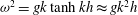 ${\it\omega}^{2}=gk\tanh kh\approx gk^{2}h$
or
${\it\omega}^{2}=gk\tanh kh\approx gk^{2}h$
or
 ${\it\omega}=k\sqrt{gh}$
. Hence the frequency closure requirement given in (2.1) can written in the following form:
${\it\omega}=k\sqrt{gh}$
. Hence the frequency closure requirement given in (2.1) can written in the following form:
 $$\begin{eqnarray}{\bf\omega}_{1}\pm {\bf\omega}_{2}\pm \cdots \pm {\bf\omega}_{m+1}=0=\sqrt{gh}(k_{1}\pm k_{2}\pm \cdots \pm k_{m+1}),\quad m\geqslant 1.\end{eqnarray}$$
This shows that for one-dimensional interactions the resonance conditions will be satisfied for any order. It is true, of course, for the dominating class III Bragg resonance, which relates to wave triads, but it also relates to quartets, quintets and so on. This fact explains why models that in practice neglect bottom components or simulate triad interaction by degenerating quartet interaction models can exhibit a good physical behaviour. In two-dimensional interactions the resonant condition (2.2) will not be closed without a bottom component. Nevertheless, for very small bottom slopes its neglect may be justified, as the bottom depth will be composed mainly by very small-wavenumber components.
There are various possibilities to fulfill the nonlinear resonance conditions (2.2) exactly. Two elementary possibilities are to be considered in this discussion for both intermediate and shallow water depths: one-dimensional superharmonic self-interaction and a subharmonic interaction. First, let us consider superharmonic self-interaction, i.e. a monochromatic wave interacting with itself to generate a wave at double frequency (see figure 1 a,c). In this case the resonance conditions (2.2) take the form
 $$\begin{eqnarray}\displaystyle 2{\bf\omega}_{1}-{\bf\omega}_{3}=0,\quad 2k_{1}-k_{3}\pm K=0. & & \displaystyle\end{eqnarray}$$
The resonating superharmonic frequency
 ${\bf\omega}_{3}$
is found to be the second harmonic (
${\bf\omega}_{3}$
is found to be the second harmonic (
 $2{\bf\omega}_{1}$
). Its wavenumber
$2{\bf\omega}_{1}$
). Its wavenumber
 $k_{3}=k_{3}({\it\omega}_{3})$
can be easily found using the dispersion relation
$k_{3}=k_{3}({\it\omega}_{3})$
can be easily found using the dispersion relation
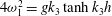 $4{\it\omega}_{1}^{2}=gk_{3}\tanh k_{3}h$
, and the required bottom component for closing the resonance condition is hence given by
$4{\it\omega}_{1}^{2}=gk_{3}\tanh k_{3}h$
, and the required bottom component for closing the resonance condition is hence given by
 $K=k_{3}-2k_{1}$
. In shallow water the resulting bottom component
$K=k_{3}-2k_{1}$
. In shallow water the resulting bottom component
 $K$
will be zero.
$K$
will be zero.
Second, let us consider a one-dimensional subharmonic interaction between two forward-propagating waves of the third and second harmonics generating a forward-propagating first harmonic wave. The closure of the frequency resonance condition can be written as
 $$\begin{eqnarray}\displaystyle {\bf\omega}_{1}-{\bf\omega}_{2}-{\bf\omega}_{3}={\it\omega}_{1}-3{\it\omega}_{1}+2{\it\omega}_{1}=0. & & \displaystyle\end{eqnarray}$$
The wavenumbers
 $k_{1}$
,
$k_{1}$
,
 $k_{2}$
and
$k_{2}$
and
 $k_{3}$
can be calculated using the dispersion relation with the frequencies
$k_{3}$
can be calculated using the dispersion relation with the frequencies
 ${\it\omega}_{1}$
,
${\it\omega}_{1}$
,
 $3{\it\omega}_{1}$
and
$3{\it\omega}_{1}$
and
 $2{\it\omega}_{1}$
, respectively. The required bottom component for closing the resonance condition is hence given by
$2{\it\omega}_{1}$
, respectively. The required bottom component for closing the resonance condition is hence given by
 $$\begin{eqnarray}K=k_{2}-k_{3}-k_{1},\end{eqnarray}$$
which in shallow water will again be zero (see figure 1 b,d). These two types of interactions will also be investigated numerically in § 5.

Figure 1. Geometric construction of class III Bragg unidirectional resonance triad interactions. (a,c) Superharmonic self-interaction (
 $k_{1}+k_{1}$
) generating a second harmonic wave (
$k_{1}+k_{1}$
) generating a second harmonic wave (
 $k_{3}$
) in intermediate (a) and shallow (c) water depths. (b,d) Subharmonic interaction (
$k_{3}$
) in intermediate (a) and shallow (c) water depths. (b,d) Subharmonic interaction (
 $k_{2}-k_{3}$
) generating a long wave (
$k_{2}-k_{3}$
) generating a long wave (
 $k_{1}$
) in intermediate (b) and shallow (d) water depths. Black arrows represent interacting wave components and the generated wave. Blue arrows represent the bottom component
$k_{1}$
) in intermediate (b) and shallow (d) water depths. Black arrows represent interacting wave components and the generated wave. Blue arrows represent the bottom component
 $(K_{bot})$
where required for closing the wave resonance condition. The circles represent all wavenumber solutions that satisfy the frequency resonance closure. The problem parameters and calculated values are given in table 1. In contrast to intermediate water depth interactions, unidirectional shallow water interaction conditions can be satisfied without requiring a bottom component. This indicates a very different physical behaviour.
$(K_{bot})$
where required for closing the wave resonance condition. The circles represent all wavenumber solutions that satisfy the frequency resonance closure. The problem parameters and calculated values are given in table 1. In contrast to intermediate water depth interactions, unidirectional shallow water interaction conditions can be satisfied without requiring a bottom component. This indicates a very different physical behaviour.
Table 1. Wavenumbers, frequencies and relative water depths for the interacting waves in figure 1, for both intermediate and shallow water.

3 Derivation of the deterministic evolution equations
The present section describes the elimination of the vertical axis and the derivation of the deterministic nonlinear spectral amplitude evolution equations. The method chosen here follows closely the one used by Bredmose et al. (Reference Bredmose, Agnon, Madsen and Schaffer2005). This method was chosen in order to better account for the nonlinear quadratic interactions. It consists of some minor augmentations that include the dissipation of energy and slow time evolution.
3.1 Derivation of the Dirichlet to Neumann operator and the approximate boundary conditions
The equations governing the irrotational flow of an incompressible inviscid fluid with a free surface are given as
 $$\begin{eqnarray}\displaystyle & \displaystyle {\rm\nabla}^{2}{\it\phi}+{\it\phi}_{zz}=0,\quad -h<z<{\it\eta}, & \displaystyle\end{eqnarray}$$
 $$\begin{eqnarray}\displaystyle & \displaystyle {\it\phi}_{z}-\boldsymbol{{\rm\nabla}}{\it\phi}\boldsymbol{\cdot }\boldsymbol{{\rm\nabla}}{\it\eta}-{\it\eta}_{t}=0,\quad z={\it\eta}, & \displaystyle\end{eqnarray}$$
 $$\begin{eqnarray}\displaystyle & \displaystyle {\it\phi}_{t}+g{\it\eta}+((\boldsymbol{{\rm\nabla}}{\it\phi})^{2}+{\it\phi}_{z}^{2})/2=0,\quad z={\it\eta}, & \displaystyle\end{eqnarray}$$
 $$\begin{eqnarray}\displaystyle & \displaystyle {\it\phi}_{z}+\boldsymbol{{\rm\nabla}}h\boldsymbol{\cdot }\boldsymbol{{\rm\nabla}}{\it\phi}=0,\quad z=-h. & \displaystyle\end{eqnarray}$$
 ${\it\phi}$
. Equations (3.2) and (3.3) are the kinematic and dynamic free surface boundary conditions, respectively. Equation (3.4) describes the free-slip bottom boundary condition. The coordinate system is Cartesian, where
${\it\phi}$
. Equations (3.2) and (3.3) are the kinematic and dynamic free surface boundary conditions, respectively. Equation (3.4) describes the free-slip bottom boundary condition. The coordinate system is Cartesian, where
 $z$
is zero at the undisturbed water level and points upwards, while the
$z$
is zero at the undisturbed water level and points upwards, while the
 $x$
and
$x$
and
 $y$
axes are in the onshore and longshore directions, respectively. Finally,
$y$
axes are in the onshore and longshore directions, respectively. Finally,
 $h$
represents the water depth,
$h$
represents the water depth,
 ${\it\eta}$
is the surface elevation, subscripts denote partial differentiation by
${\it\eta}$
is the surface elevation, subscripts denote partial differentiation by
 $z$
or
$z$
or
 $t$
, and the horizontal gradient operator is represented by
$t$
, and the horizontal gradient operator is represented by
 $\boldsymbol{{\rm\nabla}}$
.
$\boldsymbol{{\rm\nabla}}$
.
For the purpose of eliminating the vertical axis, the velocity potential is expanded as a series in
 $z$
as
$z$
as
 $$\begin{eqnarray}{\it\phi}(x,z,t)=\mathop{\sum }_{n=0}^{\infty }z^{n}{\it\phi}_{n}(x,t),\end{eqnarray}$$
with
 ${\it\phi}_{0}$
and
${\it\phi}_{0}$
and
 ${\it\phi}_{1}$
describing the velocity potential and the vertical speed at the free surface, respectively:
${\it\phi}_{1}$
describing the velocity potential and the vertical speed at the free surface, respectively:
 $$\begin{eqnarray}\displaystyle & \displaystyle {\it\phi}_{0}={\it\phi}(x,0,t)={\it\Phi}, & \displaystyle\end{eqnarray}$$
 $$\begin{eqnarray}\displaystyle & \displaystyle {\it\phi}_{1}=w(x,0,t)=W. & \displaystyle\end{eqnarray}$$
 $$\begin{eqnarray}{\it\phi}_{n+2}=-{\rm\nabla}^{2}{\it\phi}_{n}/((n+1)(n+2)),\end{eqnarray}$$
allowing the velocity potential to be expressed as
 $$\begin{eqnarray}{\it\phi}(x,z,t)=\mathop{\sum }_{n=0}^{\infty }(-1)^{n}\frac{z^{2n}{\rm\nabla}^{2n}}{(2n)!}{\it\Phi}+(-1)^{n}\frac{z^{2n+1}{\rm\nabla}^{2n}}{(2n+1)!}W.\end{eqnarray}$$
The operator
 $\boldsymbol{{\rm\nabla}}$
is treated as a quasi-differential operator; it has a value only if it operates on the other terms. For simplification, the two infinite sums in (3.9) can be described using Taylor series to yield
$\boldsymbol{{\rm\nabla}}$
is treated as a quasi-differential operator; it has a value only if it operates on the other terms. For simplification, the two infinite sums in (3.9) can be described using Taylor series to yield
 $$\begin{eqnarray}{\it\phi}(x,z,t)=\cos (z\boldsymbol{{\rm\nabla}}){\it\Phi}+\frac{1}{\boldsymbol{{\rm\nabla}}}\sin (z\boldsymbol{{\rm\nabla}})W.\end{eqnarray}$$
By using (3.10), and by Taylor-expanding the surface boundary conditions around
 $z=0$
, and after using linear transformations in the nonlinear part, the boundary conditions become
$z=0$
, and after using linear transformations in the nonlinear part, the boundary conditions become
 $$\begin{eqnarray}\sin (h\boldsymbol{{\rm\nabla}})\boldsymbol{{\rm\nabla}}{\it\Phi}+\cos (h\boldsymbol{{\rm\nabla}})W=-(\boldsymbol{{\rm\nabla}}h)\boldsymbol{\cdot }\{(\boldsymbol{{\rm\nabla}}\cos (h\boldsymbol{{\rm\nabla}}){\it\Phi})-\sin (h\boldsymbol{{\rm\nabla}})W\},\end{eqnarray}$$
 $$\begin{eqnarray}-W-\frac{1}{g}{\it\phi}_{tt}+{\it\varepsilon}\left[-\frac{1}{2g^{3}}({\it\phi}_{t}^{2})_{ttt}+\frac{1}{2g^{3}}({\it\phi}_{tt}^{2})_{t}-\frac{1}{g}((\boldsymbol{{\rm\nabla}}{\it\phi})^{2})_{t}-\frac{1}{g}{\it\phi}_{t}{\rm\nabla}^{2}{\it\phi}\right]=O({\it\varepsilon}^{2}),\quad z=0,\end{eqnarray}$$
 $$\begin{eqnarray}g{\it\eta}+{\it\phi}_{t}+{\it\varepsilon}\left[\frac{1}{2}(\boldsymbol{{\rm\nabla}}{\it\phi})^{2}+\frac{1}{2g^{2}}({\it\phi}_{t}^{2})_{tt}-\frac{1}{2g^{2}}{\it\phi}_{tt}^{2}\right]=O({\it\varepsilon}^{2}),\quad z=0.\end{eqnarray}$$
These relations will be used for the derivation of the deterministic evolution equations for the velocity potential.
3.2 Constructing the problem in terms of spectral harmonics
Following a Wentzel–Kramers–Brillouin (WKB) approach, two time scales,
 $t_{0}$
and
$t_{0}$
and
 $t_{1}$
, are introduced. The term
$t_{1}$
, are introduced. The term
 $t_{0}$
corresponds to a fast time scale that is proportional to the leading-order oscillatory motion of the flow, while
$t_{0}$
corresponds to a fast time scale that is proportional to the leading-order oscillatory motion of the flow, while
 $t_{1}$
corresponds to slower time evolutions of the wave amplitude. For brevity, the subscript in the fast time scale is dropped
$t_{1}$
corresponds to slower time evolutions of the wave amplitude. For brevity, the subscript in the fast time scale is dropped
 $(t=t_{0})$
. The surface elevation and the velocity potential on the surface are then written in terms of the rapidly oscillating wave-like behaviour and a slowly evolving amplitude:
$(t=t_{0})$
. The surface elevation and the velocity potential on the surface are then written in terms of the rapidly oscillating wave-like behaviour and a slowly evolving amplitude:
 $$\begin{eqnarray}\displaystyle {\it\eta}(x,y,t,t_{1}) & = & \displaystyle \mathop{\sum }_{p=-N}^{N}\hat{{\it\eta}}_{p}(x,y,t_{1})\text{e}^{\text{i}{\it\omega}_{p}t}\nonumber\\ \displaystyle & = & \displaystyle \mathop{\sum }_{p=-N}^{N}\mathop{\sum }_{l=-M}^{M}a_{p,l}(x,t_{1})\text{e}^{\text{i}({\it\omega}_{p}t-\int k_{p,l}^{x}\,\text{d}x-k_{l}^{y}y)},\end{eqnarray}$$
 $$\begin{eqnarray}\displaystyle {\it\phi}(x,y,t,t_{1}) & = & \displaystyle \mathop{\sum }_{p=-N}^{N}\hat{{\it\phi}}_{p}(x,y,t_{1})\text{e}^{\text{i}{\it\omega}_{p}t}\nonumber\\ \displaystyle & = & \displaystyle \mathop{\sum }_{p=-N}^{N}\mathop{\sum }_{l=-M}^{M}b_{p,l}(x,t_{1})\text{e}^{\text{i}({\it\omega}_{p}t-\int k_{p,l}^{x}\,\text{d}x-k_{l}^{y}y)}.\end{eqnarray}$$
 ${\it\omega}_{p}=p{\it\omega}_{1}$
represents the wave frequency, with
${\it\omega}_{p}=p{\it\omega}_{1}$
represents the wave frequency, with
 ${\it\omega}_{1}$
representing the lowest considered wave frequency. The terms
${\it\omega}_{1}$
representing the lowest considered wave frequency. The terms
 $k_{p,l}^{x}$
and
$k_{p,l}^{x}$
and
 $k_{l}^{y}$
are the onshore and longshore wavenumbers, respectively, with the wavenumber vector defined as
$k_{l}^{y}$
are the onshore and longshore wavenumbers, respectively, with the wavenumber vector defined as
 $\boldsymbol{k}_{p,l}=(k_{p,l}^{x},k_{l}^{y})^{\text{T}}$
.
$\boldsymbol{k}_{p,l}=(k_{p,l}^{x},k_{l}^{y})^{\text{T}}$
.
In order to retain a real value for the surface elevation, it is clear that
 $a_{-p,l}=a_{p,l}^{\ast }$
and
$a_{-p,l}=a_{p,l}^{\ast }$
and
 $a_{0,l}\in R$
. The same applies for the amplitudes of the velocity potential. From here the derivation of Bredmose et al. (Reference Bredmose, Agnon, Madsen and Schaffer2005) is followed to obtain
$a_{0,l}\in R$
. The same applies for the amplitudes of the velocity potential. From here the derivation of Bredmose et al. (Reference Bredmose, Agnon, Madsen and Schaffer2005) is followed to obtain
 $$\begin{eqnarray}\displaystyle & & \displaystyle \left(\tan (h\boldsymbol{{\rm\nabla}})\boldsymbol{{\rm\nabla}}+\frac{{\it\omega}_{p}^{2}}{g}\right)\hat{{\it\phi}}_{p}=2\frac{\text{i}{\it\omega}_{p}}{g}\frac{\partial }{\partial t_{1}}\hat{{\it\phi}}_{p}-\sec (h\boldsymbol{{\rm\nabla}})(\boldsymbol{{\rm\nabla}}h)\nonumber\\ \displaystyle & & \displaystyle \quad \times \left\{\!(\cos (h\boldsymbol{{\rm\nabla}})\boldsymbol{{\rm\nabla}}\hat{{\it\phi}}_{p})-\sin (h\boldsymbol{{\rm\nabla}})\frac{{\it\omega}_{p}^{2}}{g}\hat{{\it\phi}}_{p}\right\}-{\it\varepsilon}\mathop{\sum }_{s=p-N}^{N}Y_{s,p-s}^{(2)}\hat{{\it\phi}}_{s}\hat{{\it\phi}}_{p-s}+O({\it\varepsilon}^{2}),\end{eqnarray}$$
 $$\begin{eqnarray}\displaystyle Y_{s,p-s}^{(2)} & = & \displaystyle \frac{\text{i}}{2g^{3}}{\it\omega}_{s}^{2}{\it\omega}_{p-s}^{2}{\it\omega}_{p}-\frac{\text{i}}{2g^{3}}{\it\omega}_{s}{\it\omega}_{p-s}{\it\omega}_{p}^{3}\nonumber\\ \displaystyle & & \displaystyle -\,\frac{\text{i}}{g}{\it\omega}_{p}\boldsymbol{{\rm\nabla}}_{s}\boldsymbol{\cdot }\boldsymbol{{\rm\nabla}}_{p-s}-\frac{\text{i}}{2g}{\it\omega}_{p-s}\boldsymbol{{\rm\nabla}}_{s}^{2}-\frac{\text{i}}{2g}{\it\omega}_{s}\boldsymbol{{\rm\nabla}}_{p-s}^{2}.\end{eqnarray}$$
The horizontal derivative operators
 $\boldsymbol{{\rm\nabla}}_{s}$
and
$\boldsymbol{{\rm\nabla}}_{s}$
and
 $\boldsymbol{{\rm\nabla}}_{p-s}$
are defined as ones that operate only on
$\boldsymbol{{\rm\nabla}}_{p-s}$
are defined as ones that operate only on
 ${\it\phi}_{s}$
and
${\it\phi}_{s}$
and
 ${\it\phi}_{p-s}$
, respectively.
${\it\phi}_{p-s}$
, respectively.
Equation (3.16) is the same as in the work of Bredmose et al. (Reference Bredmose, Agnon, Madsen and Schaffer2005), with the exception of the term that accounts for slow time effects. The dispersion relation can be obtained from (3.16) while accounting for quadratic nonlinear effects (see appendix A). This work will remain with the common dispersion relation approximation for linear water waves propagating over horizontal bottom.
3.3 Splitting the dispersion operator
The spectral evolution equations derived in the previous section incorporate all wave propagation. In many wave shoaling scenarios, the vast majority of the wave energy propagates to the shore direction with negligible reflection. Formulating the evolution equations for such shoaling scenarios will significantly reduce the computational costs as the model behaves in a hyperbolic manner. In order to apply such a simplification, it will be helpful to start with the case of linear wave propagation with constant depth. In this case (3.16) takes the form
 $$\begin{eqnarray}\left(\tan (h\boldsymbol{{\rm\nabla}})\boldsymbol{{\rm\nabla}}+\frac{{\it\omega}_{p}^{2}}{g}\right)\hat{{\it\phi}}_{p}={\it\alpha}_{p}\hat{{\it\phi}}_{p},\end{eqnarray}$$
where
 ${\it\alpha}_{p}$
represents the linear dissipation coefficient. For the case of no lateral bottom changes, the lateral wavenumbers would remain constant and the wave field evolves only in the onshore direction
${\it\alpha}_{p}$
represents the linear dissipation coefficient. For the case of no lateral bottom changes, the lateral wavenumbers would remain constant and the wave field evolves only in the onshore direction
 $x$
. For this case, the dispersion operator in (3.18) is rewritten in the form
$x$
. For this case, the dispersion operator in (3.18) is rewritten in the form
 $$\begin{eqnarray}\left(\tan (h\boldsymbol{{\rm\nabla}})\boldsymbol{{\rm\nabla}}+\frac{{\it\omega}_{p}^{2}}{g}\right)\equiv \frac{\partial _{x}+\text{i}k_{p,l}^{x}+D_{p,l}}{H},\end{eqnarray}$$
with the dissipation term
 $D_{p,l}$
defined as
$D_{p,l}$
defined as
 $$\begin{eqnarray}D_{p,l}={\it\alpha}_{p}H.\end{eqnarray}$$
Equation (3.19) can be solved to yield a definition for the operator
 $H$
:
$H$
:
 $$\begin{eqnarray}H=\frac{\partial _{x}+\text{i}k_{p,l}^{x}+D_{p,l}}{\displaystyle \tan (h\boldsymbol{{\rm\nabla}})\boldsymbol{{\rm\nabla}}+\frac{{\it\omega}_{p}^{2}}{g}}.\end{eqnarray}$$
Applying (3.19) to (3.16) results in a hyperbolic model with pseudo-differential higher-order terms:
 $$\begin{eqnarray}\displaystyle (\partial _{x}+\text{i}k_{p,l}^{x}+D_{p,l})\hat{{\it\phi}}_{p} & = & \displaystyle 2H\frac{\text{i}{\it\omega}_{p}}{g}\frac{\partial \hat{{\it\phi}}_{p}}{\partial t_{1}}-H\sec (h\boldsymbol{{\rm\nabla}})(\boldsymbol{{\rm\nabla}}h)\{\sec (h\boldsymbol{{\rm\nabla}})\boldsymbol{{\rm\nabla}}\hat{{\it\phi}}_{p}\}\nonumber\\ \displaystyle & & \displaystyle -\,{\it\varepsilon}\mathop{\sum }_{s=p-N}^{N}HY_{s,p-s}^{(2)}\hat{{\it\phi}}_{s}\hat{{\it\phi}}_{p-s}.\end{eqnarray}$$
Here, the solution for
 ${\it\omega}_{p}^{2}/g$
on the right-hand side was approximated.
${\it\omega}_{p}^{2}/g$
on the right-hand side was approximated.
Next, the expression for the bed slope term, which contains derivatives of the bottom depth, is replaced using the common mild-slope result
 $$\begin{eqnarray}-\frac{C_{g,p}^{\prime }}{2C_{g,p}},\end{eqnarray}$$
where
 $C_{g,p}$
is the group speed and
$C_{g,p}$
is the group speed and
 $C_{g,p}^{\prime }$
is the derivative of the group speed in the onshore direction for the spectral component
$C_{g,p}^{\prime }$
is the derivative of the group speed in the onshore direction for the spectral component
 $p$
. Finally, the evolution equation for the Fourier amplitude of velocity potential takes the form
$p$
. Finally, the evolution equation for the Fourier amplitude of velocity potential takes the form
 $$\begin{eqnarray}\displaystyle \left(\frac{1}{C_{g,p}}\frac{\partial }{\partial t_{1}}+\partial _{x}+\text{i}k_{p,l}^{x}+\frac{C_{g,p}^{\prime }}{2C_{g,p}}+D_{p,l}\right)\hat{{\it\phi}}_{p}=-{\it\varepsilon}\mathop{\sum }_{s=p-N}^{N}HY_{s,p-s}^{(2)}\hat{{\it\phi}}_{s}\hat{{\it\phi}}_{p-s}. & & \displaystyle\end{eqnarray}$$
Note that if one substitutes the derivative operator with the leading-order spectral component derivative
 $(\boldsymbol{{\rm\nabla}}=\text{i}k_{p,l})$
into the left-hand side of (3.23), the results will not exactly match. They will be almost identical in shallow water where the contribution of the bed slope term is most significant, but will differ in intermediate water. Thee is a further discussion on this in appendix B.
$(\boldsymbol{{\rm\nabla}}=\text{i}k_{p,l})$
into the left-hand side of (3.23), the results will not exactly match. They will be almost identical in shallow water where the contribution of the bed slope term is most significant, but will differ in intermediate water. Thee is a further discussion on this in appendix B.
3.4 Expanding in the lateral direction
Equation (3.24) still depends on the lateral direction. As the model is derived for the case when the lateral effects are assumed to be negligible, the dependence of the spectral amplitude on lateral direction can be removed. By assuming that
 $k_{l}^{y}$
remains constant in the propagation of the wave field, the spectral amplitude is again Fourier-transformed, this time eliminating the dependence of the
$k_{l}^{y}$
remains constant in the propagation of the wave field, the spectral amplitude is again Fourier-transformed, this time eliminating the dependence of the
 $y$
axis from the spectral amplitudes. This is done by expanding the left-hand side of (3.24) using the right-hand side of (3.15) to yield
$y$
axis from the spectral amplitudes. This is done by expanding the left-hand side of (3.24) using the right-hand side of (3.15) to yield
 $$\begin{eqnarray}\displaystyle \mathop{\sum }_{l=-M}^{M}\left\{\frac{\partial b_{p,l}}{\partial x}\right\}\text{e}^{-\text{i}(\int k_{p,l}^{x}\,\text{d}x+k_{l}^{y}y)} & = & \displaystyle -\frac{C_{g,p}^{\prime }}{2C_{g,p}}\hat{{\it\phi}}_{p}-D_{p}\hat{{\it\phi}}_{p}-\frac{1}{C_{g,p}}\frac{\partial }{\partial t_{1}}\hat{{\it\phi}}_{p}\nonumber\\ \displaystyle & & \displaystyle -\,{\it\varepsilon}\mathop{\sum }_{s=p-N}^{N}HY_{s,p-s}^{(2)}\hat{{\it\phi}}_{s}\hat{{\it\phi}}_{p-s}.\end{eqnarray}$$
By expanding the right-hand side of this equation, and by following the approach of Bredmose et al. (Reference Bredmose, Agnon, Madsen and Schaffer2005), the final form of the deterministic evolution equation for the Fourier amplitude of the velocity potential independent of the
 $y$
component is
$y$
component is
 $$\begin{eqnarray}\displaystyle & & \displaystyle \frac{1}{C_{g,p}}\frac{\partial b_{p,l}}{\partial t_{1}}+\frac{\partial b_{p,l}}{\partial x}=-\frac{C_{g,p}^{\prime }}{2C_{g,p}}b_{p,l}-D_{p,l}b_{p,l}\nonumber\\ \displaystyle & & \displaystyle \quad -\,{\it\varepsilon}\left(\mathop{\sum }_{s=p-N}^{N}\mathop{\sum }_{u=\text{max}\{l-M,-M\}}^{\text{min}\{l+M,M\}}H{\tilde{Y}}_{s,p-s,u,l-u}^{(2)}b_{s,u}b_{p-s,l-u}\text{e}^{-\text{i}\int (k_{s,u}^{x}+k_{p-s,l-u}^{x}-k_{p,l}^{x})\,\text{d}x}\right).\end{eqnarray}$$
The terms inside the nonlinear part are defined as
 $$\begin{eqnarray}\displaystyle {\tilde{Y}}_{s,p-s,u,l-u}^{(2)} & = & \displaystyle \frac{\text{i}}{2g^{3}}{\it\omega}_{s}^{2}{\it\omega}_{p-s}^{2}{\it\omega}_{p}-\frac{\text{i}}{2g^{3}}{\it\omega}_{s}{\it\omega}_{p-s}{\it\omega}_{p}^{3}+\frac{\text{i}}{g}{\it\omega}_{p}(k_{s,u}^{x}k_{p-s,l-u}^{x}+k_{s,u}^{y}k_{p-s,l-u}^{y})\nonumber\\ \displaystyle & & \displaystyle \quad +\,\frac{\text{i}}{2g}{\it\omega}_{p-s}(k_{s,u})^{2}+\frac{\text{i}}{2g}{\it\omega}_{s}(k_{p-s,l-u})^{2},\end{eqnarray}$$
 $$\begin{eqnarray}H=\frac{\partial _{x}+\text{i}k_{p,l}^{x}+D_{p,l}}{\tan (h\boldsymbol{{\rm\nabla}})\boldsymbol{{\rm\nabla}}+k_{p,l}\tanh (hk_{p,l})+\text{i}k_{p,l}(\boldsymbol{{\rm\nabla}}h)\text{sech}(k_{p,l}h)^{2}}.\end{eqnarray}$$
The term
 $\boldsymbol{{\rm\nabla}}$
can be interpreted in two ways. One is the so-called resonant model
$\boldsymbol{{\rm\nabla}}$
can be interpreted in two ways. One is the so-called resonant model
 $\boldsymbol{{\rm\nabla}}=\text{i}k_{p,l}$
as used by Agnon & Sheremet (Reference Agnon and Sheremet1997), which assumes resonance of the nonlinear components with the free wave. The other approach, which will be adopted here, is
$\boldsymbol{{\rm\nabla}}=\text{i}k_{p,l}$
as used by Agnon & Sheremet (Reference Agnon and Sheremet1997), which assumes resonance of the nonlinear components with the free wave. The other approach, which will be adopted here, is
 $\boldsymbol{{\rm\nabla}}=-\text{i}(k_{s,u}+k_{p-s,l-u})$
as used by Bredmose et al. (Reference Bredmose, Agnon, Madsen and Schaffer2005). The radial frequencies
$\boldsymbol{{\rm\nabla}}=-\text{i}(k_{s,u}+k_{p-s,l-u})$
as used by Bredmose et al. (Reference Bredmose, Agnon, Madsen and Schaffer2005). The radial frequencies
 ${\it\omega}_{i}$
are calculated using the dispersion relation for the flat bottom case.
${\it\omega}_{i}$
are calculated using the dispersion relation for the flat bottom case.
The evolution equation (3.26) for the velocity potential spectrum will be written in terms of amplitudes of
 ${\it\eta}$
while retaining accuracy of
${\it\eta}$
while retaining accuracy of
 $O({\it\varepsilon}^{2})$
. The approach used is that of Agnon & Sheremet (Reference Agnon and Sheremet1997), with the correction of Eldeberky & Madsen (Reference Eldeberky and Madsen1999). The second-order relation between
$O({\it\varepsilon}^{2})$
. The approach used is that of Agnon & Sheremet (Reference Agnon and Sheremet1997), with the correction of Eldeberky & Madsen (Reference Eldeberky and Madsen1999). The second-order relation between
 $\hat{{\it\phi}}_{p}$
and
$\hat{{\it\phi}}_{p}$
and
 $\hat{{\it\eta}}_{p}$
is constructed by inserting (3.14) and (3.15) into (3.13) while using the linear relation
$\hat{{\it\eta}}_{p}$
is constructed by inserting (3.14) and (3.15) into (3.13) while using the linear relation
 $\hat{{\it\phi}}_{p}=(\text{i}g/{\it\omega}_{p})\hat{{\it\eta}}_{p}$
in the nonlinear terms without a reduction in accuracy. By following the approach of Agnon & Sheremet (Reference Agnon and Sheremet1997) and Eldeberky & Madsen (Reference Eldeberky and Madsen1999) the evolution equation for the surface elevation amplitude is obtained in the form
$\hat{{\it\phi}}_{p}=(\text{i}g/{\it\omega}_{p})\hat{{\it\eta}}_{p}$
in the nonlinear terms without a reduction in accuracy. By following the approach of Agnon & Sheremet (Reference Agnon and Sheremet1997) and Eldeberky & Madsen (Reference Eldeberky and Madsen1999) the evolution equation for the surface elevation amplitude is obtained in the form
 $$\begin{eqnarray}\displaystyle & & \displaystyle \frac{1}{C_{g,p}}\frac{\partial a_{p,l}}{\partial t_{1}}+\frac{\partial a_{p,l}}{\partial x}+\frac{C_{g,p}^{\prime }}{2C_{g,p}}a_{p,l}+D_{p,l}a_{p,l}\nonumber\\ \displaystyle & & \displaystyle \quad =-{\it\varepsilon}\text{i}\mathop{\sum }_{s=p-N}^{N}\mathop{\sum }_{u=\text{max}\{l-M,-M\}}^{\text{min}\{l+M,M\}}W_{s,p-s,u,l-u}a_{s,u}a_{p-s,l-u}\text{e}^{-\text{i}\int (k_{s,u}^{x}+k_{p-s,l-u}^{x}-k_{p,l}^{x})\,\text{d}x},\end{eqnarray}$$
where
 $$\begin{eqnarray}\displaystyle & \displaystyle T_{s,p-s}^{(2)}=\frac{g^{2}k_{s}k_{p-s}}{2{\it\omega}_{p}{\it\omega}_{s}{\it\omega}_{p-s}}-\frac{1}{2}{\it\omega}_{p}+\frac{{\it\omega}_{s}{\it\omega}_{p-s}}{2{\it\omega}_{p}}, & \displaystyle\end{eqnarray}$$
 $$\begin{eqnarray}\displaystyle & \displaystyle W_{s,p-s}=-\frac{{\it\omega}_{p}}{g}(k_{s,u}^{x}+k_{p-s,l-u}^{x}-k_{p,l}^{x})T_{s,p-s}^{(2)}+g\frac{{\it\omega}_{p}}{{\it\omega}_{s}{\it\omega}_{p-s}}H{\tilde{Y}}_{s,p-s}^{(2)}. & \displaystyle\end{eqnarray}$$
Equation (3.29) is essentially the model derived by Bredmose et al. (Reference Bredmose, Agnon, Madsen and Schaffer2005), but it also incorporates dissipation and slow time evolution. Note that the derivation in this section resulted in a quasi-two-dimensional hyperbolic model, hence diffraction, backscattering or reflection are not taken into account. Still, the model is aimed for the advancement of the wave action equation to account for nonlinear triad interactions, which are also hyperbolic in their nature and commonly do not take these effects into account.
4 Stochastic model
The deterministic model given in (3.29) can be used for calculation of nonlinear wave shoaling. Nevertheless, the deterministic approach has several limitations that may make it problematic for some applications. In order to solve the model for a realistic scenario, numerical methods should be used. For this purpose the calculation grid should be defined containing several grid points per wavelength (Nyquist limitation), resulting in a requirement for a grid point every few metres. As the calculation area grows larger, the computational effort required becomes enormous, and this approach is limited by the lack of adequate computer resources. Another limitation of the deterministic calculation is the lack of a simplified physical source term for including the injection of wind energy into the waves (or in some cases its extraction) and the lack of adequate deterministic information about the wind flow above the water. Hence, for a large calculation region the wind-generated waves are hard to account for using such an approach. In addition, for forecasting purposes, the system is very chaotic, a fact that reduces its ability to serve as a long-time forecasting tool.
The above reasons gave rise to the utilization of ensemble-averaged stochastic models. The wave energy (or action) variance is advected in these models while the wave phase is averaged, the characteristic length scale becomes much larger than the wavelength. Hence, the model leaps over the Nyquist limitation and can have a grid spacing of quite a few wavelengths. Empirical models of wave growth (and decay) were constructed for such models and the ensemble averaging resulted in the formulation being more stable for forecasting purposes. Hence, stochastic wave action models are the main tool for wave hindcasting, nowcasting and forecasting of surface gravity waves in larger domains.
4.1 Deriving the stochastic evolution equations
The aim of this section is to derive coupled equations for the energy spectrum and bispectrum and to combine them into a one-equation model for the forward-propagating wave field. This is done in the manner of Agnon & Sheremet (Reference Agnon and Sheremet1997) but using (3.29) as a starting point. The slow time evolution of the bispectra will be neglected. Multiplying (3.29) by the complex conjugate of
 $a_{p,l}$
while adding the result to its complex conjugate and ensemble averaging yields
$a_{p,l}$
while adding the result to its complex conjugate and ensemble averaging yields
 $$\begin{eqnarray}\displaystyle & & \displaystyle \frac{1}{C_{g,p}}\frac{\partial F_{p,l}}{\partial t_{1}}+\frac{\partial F_{p,l}}{\partial x}+\frac{C_{g,p}^{\prime }}{C_{g,p}}F_{p,l}+2D_{p,l}F_{p,l}\nonumber\\ \displaystyle & & \displaystyle \quad =-2\mathop{\sum }_{s=p-N}^{N}\mathop{\sum }_{u=\text{max}\{l-M,-M\}}^{\text{min}\{l+M,M\}}\text{Re}[(\text{i}W_{s,p-s,u,l-u}B_{s,u,p-s,l-u})\text{e}^{-\text{i}\int (k_{s,u}^{x}+k_{p-s,l-u}^{x}-k_{p,l}^{x})\,\text{d}x}],\end{eqnarray}$$
with the energy spectrum and bispectrum defined as
 $$\begin{eqnarray}\displaystyle F_{p,l}=\langle |a_{p,l}|^{2}\rangle ,\quad B_{s,u,p-s,l-u}=\langle a_{p,l}^{\ast }a_{s,u}a_{p-s,l-u}\rangle . & & \displaystyle\end{eqnarray}$$
The angular brackets
 $\langle ~\rangle$
denote the ensemble averaging operation.
$\langle ~\rangle$
denote the ensemble averaging operation.
4.2 Two- and one-equation models
The next step is to derive an evolution equation for the bispectrum. In this derivation we will ignore the slow time evolution. This topic will be left for future work. The
 $x$
derivative of the bispectrum can be constructed in the following form:
$x$
derivative of the bispectrum can be constructed in the following form:
 $$\begin{eqnarray}\frac{\text{d}B_{s,u,p-s,l-u}}{\text{d}x}=\left\langle a_{p,l}^{\ast }a_{p-s,l-u}\frac{\text{d}a_{s,u}}{\text{d}x}\right\rangle +\left\langle a_{p,l}^{\ast }a_{s,u}\frac{\text{d}a_{p-s,l-u}}{\text{d}x}\right\rangle +\left\langle a_{s,u}a_{p-s,l-u}\frac{\text{d}a_{p,l}^{\ast }}{\text{d}x}\right\rangle .\end{eqnarray}$$
Applying (3.29) to (4.3) yields
 $$\begin{eqnarray}\displaystyle & & \displaystyle \frac{\text{d}B_{s,u,p-s,l-u}}{\text{d}x}+(D_{p,l}+D_{s,u}+D_{p-s,l-u})B_{s,u,p-s,l-u}\nonumber\\ \displaystyle & & \displaystyle \qquad +\left(\frac{C_{g,p}^{\prime }}{2C_{g,p}}+\frac{C_{g,s}^{\prime }}{2C_{g,s}}+\frac{C_{g,p-s}^{\prime }}{2C_{g,p-s}}\right)B_{s,u,p-s,l-u}\nonumber\\ \displaystyle & & \displaystyle \quad =-\text{i}\left(I_{q,r,s-q,u-r,-p,l,p-s,l-u}T_{q,r,s-q,u-r,-p,l,p-s,l-u}\right.\nonumber\\ \displaystyle & & \displaystyle \qquad +\,I_{q,r,s-q,u-r,-p,l,s,u}T_{q,r,s-q,u-r,-p,l,s,u}\nonumber\\ \displaystyle & & \displaystyle \qquad +\left.I_{q,r,s-q,u-r,s,u,p-s,l-u}T_{q,r,s-q,u-r,s,u,p-s,l-u}\right),\end{eqnarray}$$
with the trispectrum components and their coefficients defined as
 $$\begin{eqnarray}\displaystyle & \displaystyle T_{q,r,s-q,u-r,-p,l,p-s,l-u}=\langle a_{q,r}a_{s-q,u-r}a_{p,l}^{\ast }a_{p-s,l-u}\rangle , & \displaystyle\end{eqnarray}$$
 $$\begin{eqnarray}\displaystyle & \displaystyle I_{q,r,s-q,u-r,-p,l,p-s,l-u}=\mathop{\sum }_{q=s-N}^{N}\mathop{\sum }_{r=\text{max}\{u-M,-M\}}^{\text{min}\{u+M,M\}}W_{q,s-q,r,u-r}\text{e}^{-\text{i}\int (k_{q,r}^{x}+k_{s-q,u-r}^{x}-k_{s,u}^{x})\,\text{d}x}. & \displaystyle\end{eqnarray}$$
Applying Benney & Saffman’s closure to (3.29) yields a solvable evolution equation set for the bispectra as follows:
 $$\begin{eqnarray}\displaystyle & & \displaystyle \frac{\text{d}B_{s,u,p-s,l-u}}{\text{d}x}+(D_{p,l}+D_{s,u}+D_{p-s,l-u})B_{s,u,p-s,l-u}\nonumber\\ \displaystyle & & \displaystyle \qquad +\,\left(\frac{C_{g,p}^{\prime }}{2C_{g,p}}+\frac{C_{g,s}^{\prime }}{2C_{g,s}}+\frac{C_{g,p-s}^{\prime }}{2C_{g,p-s}}\right)B_{s,u,p-s,l-u}\nonumber\\ \displaystyle & & \displaystyle \quad =-2\text{i}\left(W_{-s,-(p-s),u,l-u}F_{s,u}F_{p-s,l-u}+W_{p,-s,l,l-u}F_{p,l}F_{s,u}\right.\nonumber\\ \displaystyle & & \displaystyle \qquad \left.+\,W_{p,-(p-s),l,l-u}F_{p,l}F_{p-s,l-u}\right)\text{e}^{\text{i}\int (k_{s,u}^{x}+k_{p-s,l-u}^{x}-k_{p,l}^{x})\,\text{d}x}.\end{eqnarray}$$
Equations (4.1) and (4.7) make up a two-equation stochastic model, which can be used to solve the shoaling problem.
The number of permutations between wave components constructing the various bispectral components is very large. This means that the large number of differential equations represented by (4.7) results in a computationally intensive situation. In order to address this limitation, equation (4.7) is solved for
 $B_{s,u,p-s,l-u}$
. The bispectrum is assumed to be negligible in deep water, as in this region the sea is nearly Gaussian. Applying the integration factor method to (4.7) yields a solution for the bispectrum,
$B_{s,u,p-s,l-u}$
. The bispectrum is assumed to be negligible in deep water, as in this region the sea is nearly Gaussian. Applying the integration factor method to (4.7) yields a solution for the bispectrum,
 $$\begin{eqnarray}B_{s,u,p-s,l-u}=\frac{\displaystyle \int _{0}^{x}U_{s,u,p-s,l-u}\text{e}^{(\int _{0}^{x^{\prime }}-J_{s,u,p-s,l-u}\,\text{d}x^{\prime \prime })\,\text{d}x^{\prime }}}{\text{e}^{\int _{0}^{x}-J_{s,u,p-s,l-u}\,\text{d}x}},\end{eqnarray}$$
with terms
 $J$
and
$J$
and
 $U$
defined as
$U$
defined as
 $$\begin{eqnarray}\displaystyle J_{s,u,p-s,l-u}=-\left(\frac{C_{g,p}^{\prime }}{2C_{g,p}}+\frac{C_{g,s}^{\prime }}{2C_{g,s}}+\frac{C_{g,p-s}^{\prime }}{2C_{g,p-s}}\right)-(D_{p,l}+D_{s,u}+D_{p-s,l-u}), & & \displaystyle\end{eqnarray}$$
 $$\begin{eqnarray}\displaystyle U_{s,u,p-s,l-u} & = & \displaystyle -2\text{i}\left(W_{-s-(,p-s),u,l-t}F_{s,u}F_{p-s,l-u}+W_{p,-s,l,t-u}F_{p,l}F_{s,u}\right.\nonumber\\ \displaystyle & & \displaystyle \left.+\,W_{p,-(p-s),l,l-u}F_{p,l}F_{p-s,l-u}\right)\text{e}^{\text{i}\int (k_{s,u}^{x}+k_{p-s,l-u}^{x}-k_{p,l}^{x})\,\text{d}x}.\end{eqnarray}$$
Eliminating the bispectral components by substituting (4.8) into (4.1) allows a one-equation model to be formed:
 $$\begin{eqnarray}\displaystyle & & \displaystyle \frac{1}{C_{g,p}}\frac{\partial F_{p,l}}{\partial t_{1}}+\frac{\partial F_{p,l}}{\partial x}+\frac{C_{g,p}^{\prime }}{C_{g,p}}F_{p,l}+2D_{p,l}F_{p,l}\nonumber\\ \displaystyle & & \displaystyle \quad =+4\mathop{\sum }_{s=p-N}^{N}\mathop{\sum }_{u=\text{max}\{l-M,-M\}}^{\text{min}\{l+M,M\}}\text{Re}[Q_{s,p-s,u,l-u}F_{s,u}F_{p-s,l-u}\nonumber\\ \displaystyle & & \displaystyle \qquad +Q_{p,s,l,t-u}F_{p,l}F_{s,u}+Q_{p,p-s,l,l-u}F_{p,l}F_{p-s,l-u} ]W_{s,p-s,u,l-u}.\end{eqnarray}$$
The nonlinear interaction term
 $Q$
is given as
$Q$
is given as
 $$\begin{eqnarray}\displaystyle Q_{s,p-s,u,l-u} & = & \displaystyle \text{e}^{-\text{i}\int _{0}^{x}(k_{s,u}^{x}+k_{p-s,l-u}^{x}-k_{p,l}^{x})\,\text{d}x}\nonumber\\ \displaystyle & & \displaystyle \times \,\frac{\displaystyle \int _{0}^{x}W_{-s,-(p-s),u,l-u}\text{e}^{\text{i}\int (k_{s,u}^{x}+k_{p-s,l-u}^{x}-k_{p,l}^{x})\,\text{d}x}\text{e}^{(\int _{0}^{x^{\prime }}-J_{s,u,p-s,l-u}\,\text{d}x^{\prime \prime })\,\text{d}x^{\prime }}}{\text{e}^{(\int _{0}^{x}-J_{s,u,p-s,l-u}\,\text{d}x)}}.\end{eqnarray}$$
In this derivation it is assumed that the energy spectrum varies slowly, so it is taken out of the integration.
Equation (4.11) describes the one-equation model, which significantly reduces the required computational effort due to the significantly reduced number of coupled differential equations. Nevertheless, it still has a downside, as it contains non-local terms which require a solution of integrals in the
 $x$
direction. This results in difficulties for its application to wave action equation models.
$x$
direction. This results in difficulties for its application to wave action equation models.
There is one difference between the current model and that of Agnon & Sheremet (Reference Agnon and Sheremet1997) that needs to be pointed out. In the previous work the bed slope term was absorbed into the spectrum, yielding
 $$\begin{eqnarray}F_{p,l}=C_{g,p}\langle |a_{p,l}|^{2}\rangle ,\end{eqnarray}$$
and as a consequence the group velocity was taken out of the integration together with the spectrum. In deep water, the group velocity remains constant; however, as the waves enter shallow water, the group velocity starts to grow quickly, so it is no longer justifiable to take it out of the integration. Because of this approach, there is an additional term
 $J$
in the (4.12), which would not exist otherwise.
$J$
in the (4.12), which would not exist otherwise.
4.3 Localizing the nonlinear shoaling coefficient of the one-equation model
In this subsection the non-local nonlinear interaction terms will be localized following the approach of Stiassnie & Drimer (Reference Stiassnie and Drimer2006) and Toledo & Agnon (Reference Toledo and Agnon2012) for deep to intermediate water depths. This localization method will be shown to fail in shallow water. Therefore, a novel localization method will be applied in this region. The resulting approximated localized model is significantly simpler for calculation, as it does not require the numerical solution of integrations in the
 $x$
direction. It is also setting a better foundation for a possible extension to two-dimensional nonlinear interactions.
$x$
direction. It is also setting a better foundation for a possible extension to two-dimensional nonlinear interactions.
4.3.1 Deep to intermediate water depths
The non-local shoaling coefficients of the present work
 $Q$
are given in (4.12). The first step in localizing the model is to rewrite
$Q$
are given in (4.12). The first step in localizing the model is to rewrite
 $Q$
using a new variable,
$Q$
using a new variable,
 $$\begin{eqnarray}{\it\xi}(x)=\int _{0}^{x}(k_{s,u}^{x}+k_{p-s,l-u}^{x}-k_{p,l}^{x}+\text{i}J_{s,u,p-s,l-u})\,\text{d}x^{\prime },\end{eqnarray}$$
in the following manner:
 $$\begin{eqnarray}Q_{s,p-s,u,l-u}=\text{e}^{-\text{i}{\it\xi}(x)}\int _{0}^{{\it\xi}(x)}\frac{W_{-s,-(p-s),u,l-u}}{k_{s,u}^{x}+k_{p-s,l-u}^{x}-k_{p,l}^{x}+\text{i}J_{s,u,p-s,l-u}}\,\text{e}^{\text{i}{\it\xi}^{\prime }}\,\text{d}{\it\xi}^{\prime }.\end{eqnarray}$$
The nonlinear interaction coefficient (4.15) is then integrated by parts twice and transformed into
 $$\begin{eqnarray}\displaystyle Q_{s,p-s,u,l-u} & = & \displaystyle \text{e}^{-\text{i}{\it\xi}(x)}\left[\left(-\frac{\text{i}W_{-s,-(p-s),u,l-u}}{k_{s,u}^{x}+k_{p-s,l-u}^{x}-k_{p,l}^{x}+\text{i}J_{s,u,p-s,l-u}}\right.\right.\nonumber\\ \displaystyle & & \displaystyle +\left.\left.\frac{\text{d}}{\text{d}{\it\xi}^{\prime }}\frac{W_{-s,-(p-s),u,l-u}}{k_{s,u}^{x}+k_{p-s,l-u}^{x}-k_{p,l}^{x}+\text{i}J_{s,u,p-s,l-u}}\right)\text{e}^{\text{i}{\it\xi}^{\prime }}\right]_{0}^{{\it\xi}(x)}\nonumber\\ \displaystyle & & \displaystyle -\,\text{e}^{-\text{i}{\it\xi}(x)}\int _{0}^{{\it\xi}(x)}\frac{\text{d}^{2}}{\text{d}{\it\xi}^{\prime 2}}\frac{W_{-s,-(p-s),u,l-u}}{k_{s,u}^{x}+k_{p-s,l-u}^{x}-k_{p,l}^{x}+\text{i}J_{s,u,p-s,l-u}}\,\text{e}^{\text{i}{\it\xi}^{\prime }}\,\text{d}{\it\xi}^{\prime }.\end{eqnarray}$$
The integration by parts can be applied recursively to derive a series similar to the Taylor series composed of terms of increasing derivatives of the original integrand and an additional higher-order residual integral term. For an arbitrary number of integrations this series is given as
 $$\begin{eqnarray}\displaystyle & & \displaystyle \text{Re}[Q_{s,p-s,u,l-u}]=\frac{\text{d}}{\text{d}{\it\xi}}\left(\frac{W_{-s,-(p-s),u,l-u}}{k_{s,u}^{x}+k_{p-s,l-u}^{x}-k_{p,l}^{x}+\text{i}J_{s,u,p-s,l-u}}\right)\nonumber\\ \displaystyle & & \displaystyle \quad -\,\frac{\text{d}^{3}}{\text{d}{\it\xi}^{3}}\left(\frac{W_{-s,-(p-s),u,l-u}}{k_{s,u}^{x}+k_{p-s,l-u}^{x}-k_{p,l}^{x}+\text{i}J_{s,u,p-s,l-u}}\right)+\cdots \nonumber\\ \displaystyle & & \displaystyle \quad +\,(-1)^{l-1}\frac{\text{d}^{2l-1}}{\text{d}{\it\xi}^{2l-1}}\left(\frac{W_{-s,-(p-s),u,l-u}}{k_{s,u}^{x}+k_{p-s,l-u}^{x}-k_{p,l}^{x}+\text{i}J_{s,u,p-s,l-u}}\right)\nonumber\\ \displaystyle & & \displaystyle \quad +\,\text{Re}\left[\text{e}^{-\text{i}{\it\xi}}\left(-\frac{\text{i}W_{-s,-(p-s),u,l-u}\text{e}^{\text{i}{\it\xi}^{\prime }}}{k_{s,u}^{x}+k_{p-s,l-u}^{x}-k_{p,l}^{x}+\text{i}J_{s,u,p-s,l-u}}+\cdots \!\right)_{{\it\xi}^{\prime }=0}\right.\nonumber\\ \displaystyle & & \displaystyle \quad +\,\text{i}^{2l}\text{e}^{-\text{i}{\it\xi}}\int _{0}^{{\it\xi}}\frac{\text{d}^{2l}}{\text{d}{\it\xi}^{\prime 2l}}\left.\left(\frac{W_{-s,-(p-s),u,l-u}}{k_{s,u}^{x}+k_{p-s,l-u}^{x}-k_{p,l}^{x}+\text{i}J_{s,u,p-s,l-u}}\right)\text{e}^{\text{i}{\it\xi}^{\prime }}\,\text{d}{\it\xi}^{\prime }\right].\end{eqnarray}$$
The series part of (4.17) represents a non-oscillating and hence mean energy transfer component of the equation. The last term is commonly a fast oscillating function, at least in deep and intermediate water. As mean energy transfer components comprise the main interest in such models, Stiassnie & Drimer (Reference Stiassnie and Drimer2006) and Toledo & Agnon (Reference Toledo and Agnon2012) have neglected the last term. This last term is the only one that contains an integration, hence this resulted in localization of the nonlinear interaction coefficient. For a first-order approximation (i.e.
 $l=1$
), the deep to intermediate water depth nonlinear shoaling coefficient
$l=1$
), the deep to intermediate water depth nonlinear shoaling coefficient
 $Q$
can be reconstructed in the original variables by applying (4.14) to (4.16):
$Q$
can be reconstructed in the original variables by applying (4.14) to (4.16):
 $$\begin{eqnarray}\displaystyle & & \displaystyle \text{Re}[Q_{s,p-s,u,l-u}]=\text{Re}\left[\frac{-\text{i}W_{-s,-(p-s),u,l-u}}{k_{s,u}^{x}+k_{p-s,l-u}^{x}-k_{p,l}^{x}+\text{i}J_{s,u,p-s,l-u}}\right.\nonumber\\ \displaystyle & & \displaystyle \quad +\,\frac{1}{(k_{s,u}^{x}+k_{p-s,l-u}^{x}-k_{p,l}^{x}+\text{i}J_{s,u,p-s,l-u})^{2}}\frac{\text{d}W_{-s,-(p-s),u,l-u}}{\text{d}x}\nonumber\\ \displaystyle & & \displaystyle \quad -\left.\frac{W_{-s,-(p-s),u,l-u}}{(k_{s,u}^{x}+k_{p-s,l-u}^{x}-k_{p,l}^{x}+\text{i}J_{s,u,p-s,l-u})^{3}}\frac{\text{d}(k_{s,u}^{x}+k_{p-s,l-u}^{x}-k_{p,l}^{x}+\text{i}J_{s,u,p-s,l-u})}{\text{d}x}\right].\end{eqnarray}$$
The above approximation works well in deep to intermediate water. Nevertheless, as shown in § 2, for one-dimensional wave shoaling in shallow water the wavenumber triads can close the resonance condition. This changes the nature of the
 $\text{e}^{\pm \text{i}{\it\xi}(x)}$
components from oscillatory functions to constant or exponential ones. Hence, the localization method of Stiassnie & Drimer (Reference Stiassnie and Drimer2006) and Toledo & Agnon (Reference Toledo and Agnon2012) will fail in this region. Comparison between the local and non-local interaction coefficient models illustrating this concept can be seen from figures 2 and 3.
$\text{e}^{\pm \text{i}{\it\xi}(x)}$
components from oscillatory functions to constant or exponential ones. Hence, the localization method of Stiassnie & Drimer (Reference Stiassnie and Drimer2006) and Toledo & Agnon (Reference Toledo and Agnon2012) will fail in this region. Comparison between the local and non-local interaction coefficient models illustrating this concept can be seen from figures 2 and 3.

Figure 2. The localized (mean evolution, (4.15)) and non-local (oscillating, (4.18)) nonlinear interaction coefficients
 $Q_{1,1,0,0}$
. The coefficients describe the transfer of energy to the second harmonic due to the self-interaction of the first harmonic over a
$Q_{1,1,0,0}$
. The coefficients describe the transfer of energy to the second harmonic due to the self-interaction of the first harmonic over a
 $1/25$
slope from deep to intermediate water. The localized coefficient has also been plotted with a shift to the negative and positive directions in order to better present how it follows the mean evolution of the non-local coefficient. This specific coefficient relates to the problem described in § 5.1.
$1/25$
slope from deep to intermediate water. The localized coefficient has also been plotted with a shift to the negative and positive directions in order to better present how it follows the mean evolution of the non-local coefficient. This specific coefficient relates to the problem described in § 5.1.

Figure 3. Interaction coefficient for the propagation over a uniform slope from deep into shallow water. The case in question is transfer of energy to the first harmonic due to the subharmonic interaction of the third and fourth harmonics over a bottom slope of
 $1/10$
. The exact formulation (4.12) and the approximations of the nonlinear interaction term
$1/10$
. The exact formulation (4.12) and the approximations of the nonlinear interaction term
 $Q_{4,-3,0,0}$
are compared. The straight line represents the non-local value of the interaction term, and the dashed line represents the localized version. The agreement is very good until the waves enter shallow water, where the discarded integral starts to grow quickly, and the approximation starts failing. This coefficient relates to the problem described in § 5.3.
$Q_{4,-3,0,0}$
are compared. The straight line represents the non-local value of the interaction term, and the dashed line represents the localized version. The agreement is very good until the waves enter shallow water, where the discarded integral starts to grow quickly, and the approximation starts failing. This coefficient relates to the problem described in § 5.3.
The approximation for the mean energy transfer is shown to be quite good. The non-local energy transfer term is a fast oscillating function, while the localized one takes into account only the mean transfer of energy. The localized coefficient is centred around zero at the beginning but was plotted this way to show that it follows the mean change of the oscillating function. As the waves enter a shallower region, the oscillations decrease in magnitude, but the localized nonlinear term still follows the mean evolution (see figure 2).
4.3.2 Shallow water
The strongest resonant interactions occur in shallow water. In addition, very long infra-gravity waves are created due to nonlinear shoaling. These waves, which are essentially shallow water waves, have significant importance to various coastal applications from harbour agitation to sediment transport. It is therefore important to extend the validity of the model to this region. First the propagation over a monotonic slope is considered, and it is later shown how this approach can be used for variable bathymetry. In intermediate water, equation (4.18) describes the mean energy transfer, but as it enters shallow water the truncation of the last component can no longer be justified. Therefore, another approach is required in shallow water depths as well as a method for matching the intermediate and shallow water approximations.
The first step in the shallow water localization method is to approximate the integral in (4.12) under shallow water assumptions. This is done by splitting the integral into two parts, yielding its new form
 $$\begin{eqnarray}\displaystyle Q_{s,p-s,u,l-u} & = & \displaystyle \text{e}^{-\text{i}{\it\xi}(x)}\int _{0}^{{\it\xi}(x)}W_{-s,-(p-s),u,l-u}\text{e}^{\text{i}{\it\xi}^{\prime }}\,\text{d}{\it\xi}^{\prime }\nonumber\\ \displaystyle & = & \displaystyle \text{e}^{-\text{i}{\it\xi}(x)}\left(\int _{0}^{x_{0}}W_{-s,-(p-s),u,l-u}\text{e}^{\text{i}{\it\xi}^{\prime }}\,\text{d}{\it\xi}^{\prime }+\int _{x_{0}}^{x}W_{-s,-(p-s),u,l-u}\text{e}^{\text{i}{\it\xi}^{\prime }}\,\text{d}{\it\xi}^{\prime }\right)\nonumber\\ \displaystyle & = & \displaystyle (Y_{d}+Y_{s})\text{e}^{-\text{i}{\it\xi}(x)}.\end{eqnarray}$$
The term
 $Y_{s}$
represents the value of the integral from the start of the shallow water area,
$Y_{s}$
represents the value of the integral from the start of the shallow water area,
 $x_{0}$
, to the current point. The term
$x_{0}$
, to the current point. The term
 $Y_{d}$
is the value of the integral from the start of the propagation to the point where the waves enter shallow water,
$Y_{d}$
is the value of the integral from the start of the propagation to the point where the waves enter shallow water,
 $x_{0}$
. The problem with this approach is that there is knowledge only of the current point, and therefore the point
$x_{0}$
. The problem with this approach is that there is knowledge only of the current point, and therefore the point
 $x_{0}$
is unknown. By assuming that the slopes at the point
$x_{0}$
is unknown. By assuming that the slopes at the point
 $x_{0}$
and at the current point are the same and that the slope remains constant between them, by determining the depth at the point
$x_{0}$
and at the current point are the same and that the slope remains constant between them, by determining the depth at the point
 $x_{0}$
it is fully defined.
$x_{0}$
it is fully defined.
The cause of this failure is that the integral that was discarded from (4.17) starts to grow exponentially in the shallow water area. Therefore the depth at the point
 $x_{0}$
is chosen so that the absolute value of the term inside the discarded integral is equal to the absolute value of the interaction coefficient in the formulation for deep and intermediate water from (4.18). This ratio goes to zero in deep water, but starts growing exponentially as the water gets shallower. By choosing this point, it is ensured that the previous formulation still works relatively well, but it is starting to fall apart.
$x_{0}$
is chosen so that the absolute value of the term inside the discarded integral is equal to the absolute value of the interaction coefficient in the formulation for deep and intermediate water from (4.18). This ratio goes to zero in deep water, but starts growing exponentially as the water gets shallower. By choosing this point, it is ensured that the previous formulation still works relatively well, but it is starting to fall apart.
As the exact value of the term
 $Y_{d}$
at the point
$Y_{d}$
at the point
 $x_{0}$
is unknown, it will be approximated by the value of the localized interaction coefficient
$x_{0}$
is unknown, it will be approximated by the value of the localized interaction coefficient
 $Q_{s,p-s,u,l-u}$
from (4.18) at the point
$Q_{s,p-s,u,l-u}$
from (4.18) at the point
 $x_{0}$
, while adopting the bed slope from point
$x_{0}$
, while adopting the bed slope from point
 $x$
. It will be divided by the oscillating term in front of the integral
$x$
. It will be divided by the oscillating term in front of the integral
 $\text{e}^{-\text{i}{\it\xi}(x_{0})}$
to yield
$\text{e}^{-\text{i}{\it\xi}(x_{0})}$
to yield
 $$\begin{eqnarray}Y_{d}=\frac{Q_{s,p-s,u,l-u}(x_{0})}{\text{e}^{-\text{i}{\it\xi}(x_{0})}}.\end{eqnarray}$$
Equation (4.20) is multiplied by the value of the oscillating factor at the current point
 $\text{e}^{-\text{i}{\it\xi}(x)}$
to obtain
$\text{e}^{-\text{i}{\it\xi}(x)}$
to obtain
 $$\begin{eqnarray}\text{e}^{-\text{i}{\it\xi}(x)}Y_{d}=\text{e}^{-\text{i}[{\it\xi}(x)-{\it\xi}(x_{0})]}Q_{s,p-s,u,l-u}(x_{0}).\end{eqnarray}$$
The next step is to derive the formulation for the shallow water part of the integral
 $Y_{s}$
. The exponential term whose power is the integral of the wavenumber mismatch is absorbed into the interaction term
$Y_{s}$
. The exponential term whose power is the integral of the wavenumber mismatch is absorbed into the interaction term
 $\widetilde{W}$
, yielding
$\widetilde{W}$
, yielding
 $$\begin{eqnarray}\widetilde{W}_{-s,-(p-s),u,l-u}=W_{-s,-(p-s),u,l-u}[\text{e}^{\text{i}\int _{0}^{x}(k_{s,u}^{x}+k_{p-s,l-u}^{x}-k_{p,l}^{x})\,\text{d}x}],\end{eqnarray}$$
which leads to
 $$\begin{eqnarray}\displaystyle Y_{s} & = & \displaystyle \int _{x_{0}}^{x}\widetilde{W}_{-s,-(p-s),u,l-u}\text{e}^{\int _{x_{0}}^{x^{\prime }}-J_{s,u,p-s,l-u}\,\text{d}x^{\prime \prime }}\,\text{d}x^{\prime }\nonumber\\ \displaystyle & = & \displaystyle \int _{{\it\nu}(x_{0})}^{{\it\nu}(x)}\widetilde{W}_{-s,-(p-s),u,l-u}\text{e}^{{\it\nu}}\,\text{d}{\it\nu}^{\prime }.\end{eqnarray}$$
As before, the integral is transformed by introducing a new term
 ${\it\nu}$
and its derivative, which are given as
${\it\nu}$
and its derivative, which are given as
 $$\begin{eqnarray}{\it\nu}=\int _{x_{0}}^{x}-J_{s,u,p-s,l-u}\,\text{d}x^{\prime },\quad \text{d}{\it\nu}=-J_{s,u,p-s,l-u}\,\text{d}x.\end{eqnarray}$$
The
 ${\it\nu}$
term can be analytically determined as
${\it\nu}$
term can be analytically determined as
 $$\begin{eqnarray}\displaystyle {\it\nu} & = & \displaystyle -{\textstyle \frac{1}{2}}\ln (C_{g,p}(x)-C_{g,p}(x_{0}))\nonumber\\ \displaystyle & & \displaystyle -\,{\textstyle \frac{1}{2}}\ln (C_{g,p-s}(x)-C_{g,p-s}(x_{0}))-{\textstyle \frac{1}{2}}\ln (C_{g,s}(x)-C_{g,s}(x_{0})),\end{eqnarray}$$
by using
 $$\begin{eqnarray}-\!\int \frac{C_{g,p}^{\prime }(x)}{2C_{g,p}(x)}\,\text{d}x=-\frac{1}{2}\ln (C_{g,p}).\end{eqnarray}$$
Only the bed slope terms are considered inside the
 $J$
term and the dissipation term is omitted. The dissipation is usually empirically derived so it depends on the problem at hand. It can be inserted into the
$J$
term and the dissipation term is omitted. The dissipation is usually empirically derived so it depends on the problem at hand. It can be inserted into the
 $J$
term, provided that its integral can be determined. It should be noted that the initial value of the integral of the bed slope term at the start of the shallow water area is irrelevant, as the terms in front of and inside the integral will cancel each other out, so it is taken to be zero. Then the entire integral will be integrated by parts three times, which leads to its new form:
$J$
term, provided that its integral can be determined. It should be noted that the initial value of the integral of the bed slope term at the start of the shallow water area is irrelevant, as the terms in front of and inside the integral will cancel each other out, so it is taken to be zero. Then the entire integral will be integrated by parts three times, which leads to its new form:
 $$\begin{eqnarray}\displaystyle Y_{s} & = & \displaystyle \text{e}^{{\it\nu}}\left[\frac{\widetilde{W}_{-s,-(p-s),u,l-u}}{J_{s,u,p-s,l-u}}-\frac{\text{d}}{\text{d}{\it\nu}}\frac{\widetilde{W}_{-s,-(p-s),u,l-u}}{J_{s,u,p-s,l-u}}+\frac{\text{d}^{2}}{\text{d}{\it\nu}^{2}}\frac{\widetilde{W}_{-s,-(p-s),u,l-u}}{J_{s,u,p-s,l-u}}\right]_{{\it\nu}(x_{0})}^{{\it\nu}(x)}\nonumber\\ \displaystyle & & \displaystyle -\,\int _{{\it\nu}(x_{0})}^{{\it\nu}(x)}\frac{\text{d}^{3}}{\text{d}{\it\nu}^{\prime 3}}\left(\frac{\widetilde{W}_{-s,-(p-s),u,l-u}}{J_{s,u,p-s,l-u}}\right)\text{e}^{{\it\nu}^{\prime }}\,\text{d}{\it\nu}^{\prime }.\end{eqnarray}$$
The remaining integral cannot be solved analytically in its current form; however, the exponential term
 $\text{e}^{{\it\nu}^{\prime }}$
inside the integral can be approximated by its Taylor series
$\text{e}^{{\it\nu}^{\prime }}$
inside the integral can be approximated by its Taylor series
 $\text{e}^{{\it\nu}^{\prime }}\approx 1+{\it\nu}+{\it\nu}^{2}/2$
and, since the value of
$\text{e}^{{\it\nu}^{\prime }}\approx 1+{\it\nu}+{\it\nu}^{2}/2$
and, since the value of
 ${\it\nu}$
can be determined by using (4.25), the integral can be solved analytically. The reason that the exponential term of the wavenumber mismatch was absorbed into
${\it\nu}$
can be determined by using (4.25), the integral can be solved analytically. The reason that the exponential term of the wavenumber mismatch was absorbed into
 $W$
is because the second-order Taylor series would not be enough to approximate it and going to higher orders would be too computationally expensive. The solution of the remaining integral is given as
$W$
is because the second-order Taylor series would not be enough to approximate it and going to higher orders would be too computationally expensive. The solution of the remaining integral is given as
 $$\begin{eqnarray}\displaystyle & & \displaystyle \int _{{\it\nu}(x_{0})}^{{\it\nu}(x)}\frac{\text{d}^{3}}{\text{d}{\it\nu}^{\prime 3}}\left(\frac{\widetilde{W}_{-s,-(p-s),u,l-u}}{J_{s,u,p-s,l-u}}\right)\left(1+{\it\nu}^{\prime }+\frac{{\it\nu}^{\prime 2}}{2}\right)\text{d}{\it\nu}^{\prime }\nonumber\\ \displaystyle & & \displaystyle \quad =\left[\frac{\widetilde{W}_{-s,-(p-s),u,l-u}}{J_{s,u,p-s,l-u}}-\frac{\text{d}}{\text{d}{\it\nu}^{\prime }}\frac{\widetilde{W}_{-s,-(p-s),u,l-u}}{J_{s,u,p-s,l-u}}(1+{\it\nu}^{\prime })\right.\nonumber\\ \displaystyle & & \displaystyle \qquad \left.+\,\frac{\text{d}^{2}}{\text{d}{\it\nu}^{\prime 2}}\frac{\widetilde{W}_{-s,-(p-s),u,l-u}}{J_{s,u,p-s,l-u}}\left(1+{\it\nu}^{\prime }+\frac{{\it\nu}^{\prime 2}}{2}\right)\right]_{{\it\nu}(x_{0})}^{{\it\nu}(x)}.\end{eqnarray}$$
Some of the terms cancel out, which leads to a new formulation for
 $Y_{s}$
:
$Y_{s}$
:
 $$\begin{eqnarray}\displaystyle Y_{s} & = & \displaystyle \text{e}^{{\it\nu}}\left[\frac{\widetilde{W}_{-s,-(p-s),u,l-u}}{J_{s,u,p-s,l-u}}-\frac{\text{d}}{\text{d}{\it\nu}}\frac{\widetilde{W}_{-s,-(p-s),u,l-u}}{J_{s,u,p-s,l-u}}+\frac{\text{d}^{2}}{\text{d}{\it\nu}^{2}}\frac{\widetilde{W}_{-s,-(p-s),u,l-u}}{J_{s,u,p-s,l-u}}\right]^{{\it\nu}(x)}\nonumber\\ \displaystyle & & \displaystyle -\left[\frac{\widetilde{W}_{-s,-(p-s),u,l-u}}{J_{s,u,p-s,l-u}}-(1+{\it\nu}^{\prime })\frac{\text{d}}{\text{d}{\it\nu}}\frac{\widetilde{W}_{-s,-(p-s),u,l-u}}{J_{s,u,p-s,l-u}}\right.\nonumber\\ \displaystyle & & \displaystyle \left.+\,\left(1+{\it\nu}^{\prime }+\frac{{\it\nu}^{\prime 2}}{2}\right)\frac{\text{d}^{2}}{\text{d}{\it\nu}^{2}}\frac{\widetilde{W}_{-s,-(p-s),u,l-u}}{J_{s,u,p-s,l-u}}\right].\end{eqnarray}$$
Finally, in shallow water
 $Q$
takes the form
$Q$
takes the form
 $$\begin{eqnarray}\displaystyle Q_{s,p-s,u,l-u}(x) & = & \displaystyle \text{e}^{-\text{i}[{\it\xi}(x)-{\it\xi}(x_{0})]}(Q_{s,p-s,u,l-u}(x_{0})+Y_{s}).\end{eqnarray}$$
The terms inside (4.30) are differentiated to obtain
 $$\begin{eqnarray}\displaystyle & & \displaystyle Q_{s,p-s,u,l-u}(x)=\text{e}^{-\text{i}[{\it\xi}(x)-{\it\xi}(x_{0})]}\left\{Q_{s,p-s,u,l-u}(x_{0})+\,\left[(\text{e}^{{\it\nu}}-1)\frac{\widetilde{W}_{-s,-(p-s),u,l-u}}{J_{s,u,p-s,l-u}}\right]\vphantom{\left[\left(\frac{\displaystyle 3\left(\frac{\text{d}J_{s,u,p-s,l-u}}{\text{d}x}\right)\!\left(\frac{\text{d}\widetilde{W}_{-s,-(p-s),u,l-u}}{\text{d}x}\right)}{J_{s,u,p-s,l-u}^{4}}\right)\right]_{x_{0}}^{x}}\right.\nonumber\\ \displaystyle & & \displaystyle \quad +\,\left[(1+{\it\nu}-\text{e}^{{\it\nu}})\left(\frac{\displaystyle \frac{\text{d}\widetilde{W}_{-s,-(p-s),u,l-u}}{\text{d}x}}{J_{s,u,p-s,l-u}^{2}}-\frac{\widetilde{W}_{-s,-(p-s),u,l-u}}{J_{s,u,p-s,l-u}^{3}}\frac{\text{d}J_{s,u,p-s,l-u}}{\text{d}x}\right)\right]_{x_{0}}^{x}\nonumber\\ \displaystyle & & \displaystyle \quad -\,\left[\left(1+{\it\nu}+\frac{{\it\nu}^{2}}{2}-\text{e}^{{\it\nu}}\right)\left(\frac{\displaystyle 3\widetilde{W}_{-s,-(p-s),u,l-u}\left(\frac{\text{d}J_{s,u,p-s,l-u}}{\text{d}x}\right)^{2}}{J_{s,u,p-s,l-u}^{5}}+\frac{\displaystyle \frac{\text{d}^{2}}{\text{d}x^{2}}(\widetilde{W}_{-s,-(p-s),u,l-u})}{J_{s,u,p-s,l-u}^{3}}\vphantom{\left[\left(\frac{\displaystyle 3\left(\frac{\text{d}J_{s,u,p-s,l-u}}{\text{d}x}\right)\!\left(\frac{\text{d}\widetilde{W}_{-s,-(p-s),u,l-u}}{\text{d}x}\right)}{J_{s,u,p-s,l-u}^{4}}\right)\right]_{x_{0}}^{x}}\right.\right.\nonumber\\ \displaystyle & & \displaystyle \quad -\left.\left.\left.\frac{\displaystyle 3\left(\frac{\text{d}J_{s,u,p-s,l-u}}{\text{d}x}\right)\!\left(\frac{\text{d}\widetilde{W}_{-s,-(p-s),u,l-u}}{\text{d}x}\right)}{J_{s,u,p-s,l-u}^{4}}-\frac{\displaystyle \left(\frac{\text{d}^{2}J_{s,u,p-s,l-u}}{\text{d}x^{2}}\right)\!\widetilde{W}_{-s,-(p-s),u,l-u}}{J_{s,u,p-s,l-u}^{4}}\right)\right]_{x_{0}}^{x}\right\}.\hspace{-10.00002pt}\nonumber\\ \displaystyle & & \displaystyle\end{eqnarray}$$
The exponential terms of the integral of the wavenumber mismatch from the
 $\widetilde{W}$
terms cancel out the
$\widetilde{W}$
terms cancel out the
 $\text{e}^{-\text{i}[{\it\xi}(x)-{\it\xi}(x_{0})]}$
term to yield
$\text{e}^{-\text{i}[{\it\xi}(x)-{\it\xi}(x_{0})]}$
term to yield
 $$\begin{eqnarray}\displaystyle & & \displaystyle Q_{s,p-s,u,l-u}(x)=\text{e}^{-\text{i}[{\it\nu}(x)+{\it\xi}_{dif}]}Q_{s,p-s,u,l-u}(x_{0})+\text{e}^{-{\it\nu}(x)}\nonumber\\ \displaystyle & & \displaystyle \quad \times \,\left\{\left[(\text{e}^{{\it\nu}(x)}-1)-\frac{W_{-s,-(p-s),u,l-u}}{J_{s,u,p-s,l-u}}\right]\right.\nonumber\\ \displaystyle & & \displaystyle \quad +\left[(1+{\it\nu}-\text{e}^{{\it\nu}})\left(\frac{\widehat{W}_{-s,-(p-s),u,l-u}}{J_{s,u,p-s,l-u}^{2}}-\frac{W_{-s,-(p-s),u,l-u}}{J_{s,u,p-s,l-u}^{3}}\frac{\text{d}J_{s,u,p-s,l-u}}{\text{d}x}\right)\right]^{x}\nonumber\\ \displaystyle & & \displaystyle \quad -\left[\left(1+{\it\nu}+\frac{{\it\nu}^{2}}{2}-\text{e}^{{\it\nu}}\right)\left(\frac{\displaystyle 3W_{-s,-(p-s),u,l-u}\left(\frac{\text{d}J_{s,u,p-s,l-u}}{\text{d}x}\right)^{2}}{J_{s,u,p-s,l-u}^{5}}+\frac{\widehat{\widehat{W}}_{-s,-(p-s),u,l-u}}{J_{s,u,p-s,l-u}^{3}}\right.\right.\nonumber\\ \displaystyle & & \displaystyle \quad -\left.\left.\left.\frac{\displaystyle 3\left(\frac{\text{d}J_{s,u,p-s,l-u}}{\text{d}x}\right)\widehat{W}_{-s,-(p-s),u,l-u}}{J_{s,u,p-s,l-u}^{4}}-\frac{\displaystyle \left(\frac{\text{d}^{2}J_{s,u,p-s,l-u}}{\text{d}x^{2}}\right)\widehat{W}_{-s,-(p-s),u,l-u}}{J_{s,u,p-s,l-u}^{4}}\right)\right]_{x_{0}}^{x}\right\},\nonumber\\ \displaystyle & & \displaystyle\end{eqnarray}$$
where
 $$\begin{eqnarray}\widehat{W}_{-s,-(p-s),u,l-u}=\text{i}W_{-s,-(p-s),u,l-u}(k_{s,u}^{x}+k_{p-s,l-u}^{x}-k_{p,l}^{x})+\frac{\text{d}W_{-s,-(p-s),u,l-u}}{\text{d}x},\end{eqnarray}$$
 $$\begin{eqnarray}\displaystyle \widehat{\widehat{W}}_{-s,-(p-s),u,l-u} & = & \displaystyle \left[-(k_{s,u}^{x}+k_{p-s,l-u}^{x}-k_{p,l}^{x})^{2}+\text{i}\frac{\text{d}(k_{s,u}^{x}+k_{p-s,l-u}^{x}-k_{p,l}^{x})}{\text{d}x}\right]W_{-s,-(p-s),u,l-u}\nonumber\\ \displaystyle & & \displaystyle +\,2\text{i}\frac{\text{d}W_{-s,-(p-s),u,l-u}}{\text{d}x}(k_{s,u}^{x}+k_{p-s,l-u}^{x}-k_{p,l}^{x})+\frac{\text{d}^{2}W_{-s,-(p-s),u,l-u}}{\text{d}x^{2}},\nonumber\\ \displaystyle & & \displaystyle\end{eqnarray}$$
and
 $$\begin{eqnarray}\displaystyle {\it\xi}_{dif} & = & \displaystyle (k_{s,u}^{x}+k_{p-s,l-u}^{x}-k_{p,l}^{x})(x-x_{0})+\frac{1}{2}\frac{\partial (k_{s,u}^{x}+k_{p-s,l-u}^{x}-k_{p,l}^{x})}{\partial x}(x-x_{0})^{2}\nonumber\\ \displaystyle & & \displaystyle \!\!+\,\frac{1}{6}\frac{\partial ^{2}(k_{s,u}^{x}+k_{p-s,l-u}^{x}-k_{p,l}^{x})}{\partial x^{2}}(x-x_{0})^{3}+\frac{1}{24}\frac{\partial ^{3}(k_{s,u}^{x}+k_{p-s,l-u}^{x}-k_{p,l}^{x})}{\partial x^{3}}(x-x_{0})^{4}+\cdots \,.\nonumber\\ \displaystyle & & \displaystyle\end{eqnarray}$$
The
 ${\it\nu}$
terms were retained for brevity. This leaves one term with non-local terms in it,
${\it\nu}$
terms were retained for brevity. This leaves one term with non-local terms in it,
 ${\it\xi}(x)-{\it\xi}(x_{0})$
, and it represents the integral of the wavenumber mismatch between point
${\it\xi}(x)-{\it\xi}(x_{0})$
, and it represents the integral of the wavenumber mismatch between point
 $x_{0}$
and
$x_{0}$
and
 $x$
. This term is approximated using the Taylor series.
$x$
. This term is approximated using the Taylor series.
Finally, the two water areas are joined together using the gate function, which yields the final form of the
 $Q$
coefficient suitable for intermediate and shallow water defined as
$Q$
coefficient suitable for intermediate and shallow water defined as
 $$\begin{eqnarray}\displaystyle & & \displaystyle \text{Re}[Q_{s,p-s,u,l-u}]=\text{Re}\left[\text{e}^{-\text{i}f_{g}[{\it\nu}(x)-{\it\nu}(x_{0})+{\it\xi}_{dif}]}\left(-\frac{\text{i}W_{-s,-(p-s),u,l-u}}{k_{s,u}^{x}+k_{p-s,l-u}^{x}-k_{p,l}^{x}+\text{i}J_{s,u,p-s,l-u}}\right.\right.\nonumber\\ \displaystyle & & \displaystyle \quad +\,\frac{1}{(k_{s,u}^{x}+k_{p-s,l-u}^{x}-k_{p,l}^{x}+\text{i}J_{s,u,p-s,l-u})^{2}}\frac{\text{d}W_{-s,-(p-s),u,l-u}}{\text{d}x}\nonumber\\ \displaystyle & & \displaystyle \quad \left.\left.-\,\frac{W_{-s,-(p-s),u,l-u}}{(k_{s,u}^{x}+k_{p-s,l-u}^{x}-k_{p,l}^{x}+\text{i}J_{s,u,p-s,l-u})^{3}}\frac{\text{d}(k_{s,u}^{x}+k_{p-s,l-u}^{x}-k_{p,l}^{x}+\text{i}J_{s,u,p-s,l-u})}{\text{d}x}\right)\right]^{x+f_{g}(x_{0}-x)}\nonumber\\ \displaystyle & & \displaystyle \quad +\,\,f_{g}Q_{s,p-s,u,l-u}(x).\end{eqnarray}$$
The term
 $Q_{s,p-s,t,l-t}(x)$
is defined in (4.32). The exact formulation of the gate term is defined as
$Q_{s,p-s,t,l-t}(x)$
is defined in (4.32). The exact formulation of the gate term is defined as
 $$\begin{eqnarray}\displaystyle f_{g}=\frac{1}{2}-\frac{1}{2}\text{sgn}\left[1-\left|\frac{\text{d}^{2}}{\text{d}{\it\xi}^{2}}\frac{W_{-s,-(p-s),u,l-u}}{k_{s,u}^{x}+k_{p-s,l-u}^{x}-k_{p,l}^{x}+\text{i}J_{s,u,p-s,l-u}}\right|/|Q_{s,p-s,u,l-u}|\right]. & & \displaystyle\end{eqnarray}$$
As the water gets shallower, the term inside the discarded integral from (4.16) starts to grow exponentially and it makes discarding it result in a large error. The point that is chosen for
 $x_{0}$
is when this term is equal in magnitude to the previous localized coefficient (4.18). Although the exact ratio between these two terms is somewhat arbitrary, the ratio of one was chosen as it performed best in the examples. If the ratio is chosen to be too small, term
$x_{0}$
is when this term is equal in magnitude to the previous localized coefficient (4.18). Although the exact ratio between these two terms is somewhat arbitrary, the ratio of one was chosen as it performed best in the examples. If the ratio is chosen to be too small, term
 $Y_{s}$
will be incorrect, and if chosen too big, the term
$Y_{s}$
will be incorrect, and if chosen too big, the term
 $Y_{d}$
will be incorrect. The process used to determine the point
$Y_{d}$
will be incorrect. The process used to determine the point
 $x_{0}$
is to start from a certain depth and to slowly decrease it until the gate term becomes greater than one, thus determining the point
$x_{0}$
is to start from a certain depth and to slowly decrease it until the gate term becomes greater than one, thus determining the point
 $x_{0}$
.
$x_{0}$
.
It should be noted that it is possible for the ratio between these values to start behaving erratically when the water gets shallow. Therefore, care should be taken in very shallow water when determining the gate term. As the gate term starts to behave differently, the localized interaction coefficient for intermediate water or the term inside the discarded integral start growing in the opposite direction compared to the deep water, so this can also be used as a criterion for determining
 $f_{g}$
.
$f_{g}$
.
Often the bathymetry is characterized by many changes in the slope. This is solved by assuming at each point that it is a part of a monotonic slope propagating towards the beach. While several approximations were used in this approach, the end result matches closely the non-local nonlinear interaction term, as will be shown in the examples. The area of transition from intermediate to shallow is the most problematic one; however, this area is relatively short, and the evolution of the wave field in shallow water is described much better than in the previous models. The wave action formulation is derived and presented in appendix C.
5 Numerical examples
In order to verify the stochastic model’s validity, numerical simulations were performed using the Mathematica 9.0 software. The model used is for the one-dimensional case where all of the waves propagate in the onshore direction. Results are presented for the case of superharmonic self-interaction in intermediate water, the case of subharmonic interaction in shallow water, the propagation from deep to shallow water, a comparison with the experimental results of Luth, Klopman & Kitou (Reference Luth, Klopman and Kitou1994) and a comparison to the field measurements of Freilich & Guza (Reference Freilich and Guza1984) on the spectral evolution over a mildly sloping beach.
5.1 Superharmonic self-interaction in intermediate water depth
In this example, a monochromatic wave field is shoaling over a mildly sloping bottom, and as a result of superharmonic self-interaction, a wave of double the frequency is generated. The new model’s results are compared with the deterministic model of Bredmose et al. (Reference Bredmose, Agnon, Madsen and Schaffer2005). The problem was also modelled using the localized models of Stiassnie & Drimer (Reference Stiassnie and Drimer2006) and Toledo & Agnon (Reference Toledo and Agnon2012) for comparison purposes. These models are based on the non-local stochastic models of Agnon & Sheremet (Reference Agnon and Sheremet1997, Reference Agnon, Sheremet and Liu2000), respectively. Both use the same localization method also applied in this paper for the intermediate water region. The difference between the two models is that in the work of Stiassnie & Drimer (Reference Stiassnie and Drimer2006) the interaction coefficient corresponding to
 $W$
is assumed to be changing very slowly. This means that it is taken outside of the integration together with the spectrum before localization, while only the integral of the exponent of the wavenumber mismatch remains in the integral before the localization. In the work of Toledo & Agnon (Reference Toledo and Agnon2012) this assumption is not used and changes of the interaction term are accounted for. The present model improved the stochastic non-local model, as it accounts for faster changes of the group velocity, which were disregarded in both former models. In addition, it uses a more accurate deterministic model (Bredmose et al.
Reference Bredmose, Agnon, Madsen and Schaffer2005) as a starting point.
$W$
is assumed to be changing very slowly. This means that it is taken outside of the integration together with the spectrum before localization, while only the integral of the exponent of the wavenumber mismatch remains in the integral before the localization. In the work of Toledo & Agnon (Reference Toledo and Agnon2012) this assumption is not used and changes of the interaction term are accounted for. The present model improved the stochastic non-local model, as it accounts for faster changes of the group velocity, which were disregarded in both former models. In addition, it uses a more accurate deterministic model (Bredmose et al.
Reference Bredmose, Agnon, Madsen and Schaffer2005) as a starting point.
The bottom profile for the numerical example is defined as
 $$\begin{eqnarray}h(x)=\left\{\begin{array}{@{}lc@{}}7-0.04x\quad & x<162.5,\\ 0.5\quad & x>162.5,\end{array}\right.\end{eqnarray}$$
all of the values are given in metres. The period of the incident wave is
 $T=2$
s and the initial wave amplitude is
$T=2$
s and the initial wave amplitude is
 $A_{01}=0.02$
m, with a wave steepness of
$A_{01}=0.02$
m, with a wave steepness of
 $kA_{01}=0.0201$
. The nonlinear interaction coefficient is defined by (4.18) as the water is deep or intermediate for the whole propagation distance. As can be seen in figure 4, the current model presents a minor overprediction of the nonlinear second harmonic amplitude evolution, while the previous models present a major underprediction. Hence, the present model is shown to provide a significant improvement already for the intermediate water depths.
$kA_{01}=0.0201$
. The nonlinear interaction coefficient is defined by (4.18) as the water is deep or intermediate for the whole propagation distance. As can be seen in figure 4, the current model presents a minor overprediction of the nonlinear second harmonic amplitude evolution, while the previous models present a major underprediction. Hence, the present model is shown to provide a significant improvement already for the intermediate water depths.

Figure 4. Evolution of the wave field due to superharmonic self-interaction over a
 $1/25$
slope ending in a horizontal bar with 2 cm, and its period is 2 s. (a) First harmonic wave elevation amplitude (
$1/25$
slope ending in a horizontal bar with 2 cm, and its period is 2 s. (a) First harmonic wave elevation amplitude (
 $A_{1}$
). (b) Second harmonic wave elevation amplitude (
$A_{1}$
). (b) Second harmonic wave elevation amplitude (
 $A_{2}$
). Both amplitudes are normalized by the initial value of the first harmonic (
$A_{2}$
). Both amplitudes are normalized by the initial value of the first harmonic (
 $A_{01}$
). The oscillating line represents the deterministic solution of Bredmose et al. (Reference Bredmose, Agnon, Madsen and Schaffer2005), the dot-dashed line is the work of Stiassnie & Drimer (Reference Stiassnie and Drimer2006), the dashed line is the work of Toledo & Agnon (Reference Toledo and Agnon2012), and the thick line is the current work. Equation (4.18) was used for the simulations of the current model.
$A_{01}$
). The oscillating line represents the deterministic solution of Bredmose et al. (Reference Bredmose, Agnon, Madsen and Schaffer2005), the dot-dashed line is the work of Stiassnie & Drimer (Reference Stiassnie and Drimer2006), the dashed line is the work of Toledo & Agnon (Reference Toledo and Agnon2012), and the thick line is the current work. Equation (4.18) was used for the simulations of the current model.
5.2 Subharmonic interaction of bichromatic waves in shallow water
The nonlinear interaction between two monochromatic waves with different frequencies is inspected in this subsection in order to test the model’s capabilities to accurately represent subharmonic triad interactions. Unpublished experimental results of Stiassnie & Drimer (Reference Stiassnie and Drimer2006) were used as a benchmark. The model was compared to the models of Stiassnie & Drimer (Reference Stiassnie and Drimer2006) and Toledo & Agnon (Reference Toledo and Agnon2012) as well as to the deterministic model of Bredmose et al. (Reference Bredmose, Agnon, Madsen and Schaffer2005).
Stiassnie & Drimer’s (Reference Stiassnie and Drimer2006) experimental investigation was conducted using a wave flume 45 cm deep and 45 m long with a bottom profile given as
 $$\begin{eqnarray}h(x)=\left\{\begin{array}{@{}ll@{}}0.45\quad & x<5.64,\\ 0.45+(5.64-x)/90\quad & 5.64<x<19.41,\\ 0.297+(19.41-x)/140\quad & 19.41<x<28.09,\\ 0.235+(28.09-x)/90\quad & x>28.09,\end{array}\right.\end{eqnarray}$$
where all values are given in metres. The incident wave is a bichromatic wave with energy at periods 11 and 12 s. The model was tested for two values of the initial amplitudes: first with 1.22 cm for the incident waves and 0.02 cm for the bound wave, and second with 2.07 cm and 0.04 cm, respectively. The bichromatic waves were introduced in the experiment and the numerical calculation without a phase difference.
In this experiment, shallow waves are generated by the wavemaker, so from the beginning of the flume the shallow water localization method is used (i.e. the point
 $x_{0}$
is at the wavemaker). Therefore, the values of all energy transfer terms
$x_{0}$
is at the wavemaker). Therefore, the values of all energy transfer terms
 $Q$
at the beginning of the propagation are zero. The problem is also simulated using the deterministic model of Bredmose et al. (Reference Bredmose, Agnon, Madsen and Schaffer2005) with no phase difference at the wavemaker. The evolution of the generated harmonics is shown in figure 6, for the deterministic model (Bredmose et al.
Reference Bredmose, Agnon, Madsen and Schaffer2005) and stochastic models together with the experimental results.
$Q$
at the beginning of the propagation are zero. The problem is also simulated using the deterministic model of Bredmose et al. (Reference Bredmose, Agnon, Madsen and Schaffer2005) with no phase difference at the wavemaker. The evolution of the generated harmonics is shown in figure 6, for the deterministic model (Bredmose et al.
Reference Bredmose, Agnon, Madsen and Schaffer2005) and stochastic models together with the experimental results.

Figure 5. Difference between the non-local (solid line) and localized (dashed line) energy transfer terms for (a) the current work and (b) that of Toledo & Agnon (Reference Toledo and Agnon2012), corresponding to figure 6. The interaction coefficient in question measures the transfer of energy from the 12th and 11th harmonics to the first harmonic, through the process of subharmonic interaction. In (b) it can be seen that the localized coefficient of Toledo & Agnon (Reference Toledo and Agnon2012) is several orders of magnitude larger than the non-local coefficient, as the water is very shallow from the beginning of propagation. The localized and non-local coefficients in (b) have been plotted on different scales.

Figure 6. Amplitude evolution of a low-frequency wave due to subharmonic interaction of bichromatic waves. The energy transfer results from the subharmonic interaction of a bichromatic wave with periods of 11 and 12 s with no phase difference and with equal initial amplitudes of 1.22 cm (a) and 2.07 cm (b). Dots: unpublished experimental results of Stiassnie & Drimer (Reference Stiassnie and Drimer2006). Dashed red line and dash-dotted blue line: the localized stochastic models of Toledo & Agnon (Reference Toledo and Agnon2012) and Stiassnie & Drimer (Reference Stiassnie and Drimer2006), respectively. Thick dashed brown line: the deterministic result of Bredmose et al. (Reference Bredmose, Agnon, Madsen and Schaffer2005). Dotted brown line: ensemble average of the deterministic results of Bredmose et al. (Reference Bredmose, Agnon, Madsen and Schaffer2005). Thick black line: the current stochastic model using the shallow water approximation (4.36).
In order to show the importance of the exact phases of the interacting waves in the shallow water, an ensemble of 100 runs of the deterministic model of Bredmose et al. (Reference Bredmose, Agnon, Madsen and Schaffer2005) with randomized initial phases of the interacting waves was run 100 times. The ensemble average of the generated harmonic and the standard deviation is shown in figure 7. It can be seen that, depending on the initial phasing, the results can be very different. However, the ensemble-averaged result is in good agreement with the derived stochastic model, which shows that the new localization procedure works well in shallow water.
The localized subharmonic coefficients of Stiassnie & Drimer (Reference Stiassnie and Drimer2006) and Toledo & Agnon (Reference Toledo and Agnon2012) are shown figure in 5(b). They are orders of magnitude higher than the non-local coefficient because the localization procedure they use fails in shallow water. The coefficient obtained using the new localization procedure is shown in figure 5(a), presenting a good match to the non-local coefficient.

Figure 7. Monte Carlo averaged evolution of the generated low-frequency wave for the initial amplitude of 0.02 cm (a) and 0.04 cm (b). Thick black line: current stochastic model. Thick brown line: the averaged result of Bredmose et al. (Reference Bredmose, Agnon, Madsen and Schaffer2005). Thin brown lines: the standard deviation added or subtracted from the averaged result. Dotted line: the ensemble-averaged deterministic result of Agnon & Sheremet (Reference Agnon and Sheremet1997). Shaded area: the span of the obtained realizations using Bredmose et al. (Reference Bredmose, Agnon, Madsen and Schaffer2005).
The initial phases of the waves have a significant impact on the solution, as shown in figure 7, so extreme events should be taken into account instead in addition to ensemble-averaged results. The stochastic model shows good agreement with the deterministic and experimental results. The previous stochastic models have a very strong overshoot past a certain water depth, owing to their inability to accurately model shallow water.
5.3 Deep to shallow water nonlinear subharmonic and superharmonic interactions
The evolution of waves from deep into shallow water over a sloping bottom is presented in this subsection. The new model’s results will be compared to the stochastic models of Stiassnie & Drimer (Reference Stiassnie and Drimer2006) and Toledo & Agnon (Reference Toledo and Agnon2012). The evolution of the wave components will be compared to the deterministic model of Bredmose et al. (Reference Bredmose, Agnon, Madsen and Schaffer2005). The new model is tested for superharmonic and subharmonic interactions shoaling over a linear bottom with a slope of 10 %. The bottom profile is defined as
 $$\begin{eqnarray}h(x)=\left\{\begin{array}{@{}lc@{}}161-0.1x\quad & x<1600,\\ 1\quad & x>1600,\end{array}\right.\end{eqnarray}$$
where all values are given in metres. The periods of the interacting waves are
 $T_{1,3,4}=15,~5,~3.75$
s for the subharmonic and
$T_{1,3,4}=15,~5,~3.75$
s for the subharmonic and
 $T_{1,2}=7.5,~3.75$
s for the superharmonic self-interaction.
$T_{1,2}=7.5,~3.75$
s for the superharmonic self-interaction.

Figure 8. Comparison between the localized coefficients for three different models in the case of wave propagation from deep into shallow water over a monotonic slope. The relative water depth
 $kh$
is shown for all of the interacting wave components. The cases considered are the subharmonic interaction (a,c,e), and the case of superharmonic self-interaction (b,d,f). These coefficients govern the intensity of energy transfer to one harmonic from two other harmonics. The models used are (a,b) that of Toledo & Agnon (Reference Toledo and Agnon2012) and (c,d) that of Stiassnie & Drimer (Reference Stiassnie and Drimer2006). The equation used for the current model (e,f) is (4.36), which works in both shallow and intermediate conditions.
$kh$
is shown for all of the interacting wave components. The cases considered are the subharmonic interaction (a,c,e), and the case of superharmonic self-interaction (b,d,f). These coefficients govern the intensity of energy transfer to one harmonic from two other harmonics. The models used are (a,b) that of Toledo & Agnon (Reference Toledo and Agnon2012) and (c,d) that of Stiassnie & Drimer (Reference Stiassnie and Drimer2006). The equation used for the current model (e,f) is (4.36), which works in both shallow and intermediate conditions.
In deep to intermediate water depths, the localized coefficients follow the mean evolution of the oscillating non-local term. As the waves enter shallower depths, the original formulation fails. By using the derived shallow water localization, the range of validity of the interaction coefficients is extended to this region. Comparisons between local and non-local nonlinear interaction coefficients are presented in figure 8 together with the non-dimensional water depth of each wave component. It can be seen that, while all localized models show good agreement with the respective non-local models in deep to intermediate water, for shallow water depths the localization method in the previous works fails. It should be noted that the nature of the models is different, and therefore the magnitude of the coefficients is different for each model. The results shown in figure 8 present a measure of accuracy of the localization procedures in comparison to their non-local counterparts.
The localized stochastic models are compared to the deterministic models of Agnon et al. (Reference Agnon, Sheremet, Gonsalves and Stiassnie1993) and Kaihatu & Kirby (Reference Kaihatu and Kirby1995) for two different cases. The first case is the evolution of low (first) harmonic, due to the subharmonic interaction of two higher (third and fourth) harmonics whose amplitudes are 0.05 m. The second case is the superharmonic self-interaction of the second harmonic, whose amplitudes are 0.05 m, which generates the fourth harmonic. The evolution of harmonics for both cases is presented in figure 9.
It can be seen that previous formulations for the localized coefficients fail in shallow water. In the case of subharmonic interaction, past a certain depth the model of Toledo & Agnon (Reference Toledo and Agnon2012) overpredicts the amplitude evolution, while the model of Stiassnie & Drimer (Reference Stiassnie and Drimer2006) underpredicts the deterministic results. In the case of superharmonic interaction, the models of Stiassnie & Drimer (Reference Stiassnie and Drimer2006) and Toledo & Agnon (Reference Toledo and Agnon2012) underpredict the evolution of the amplitude. The new localization formulation shows good agreement with the deterministic model for both cases.

Figure 9. (a) The evolution of the first harmonic as a result of subharmonic interaction of the fourth and third harmonics and (b) the evolution of the fourth harmonic as a result of the self-interaction of the second harmonic. The thick black line represents the current model, the dashed line is the model of Toledo & Agnon (Reference Toledo and Agnon2012), the dash-dotted line is the model of Stiassnie & Drimer (Reference Stiassnie and Drimer2006), and the two thin lines are the deterministic models of Bredmose et al. (Reference Bredmose, Agnon, Madsen and Schaffer2005) and Agnon & Sheremet (Reference Agnon and Sheremet1997).
5.4 Monochromatic wave propagation over a bar
In this section the results of the deterministic and stochastic models are compared to the results of the experiment conducted by Luth et al. (Reference Luth, Klopman and Kitou1994). Both local and non-local formulations will be inspected. This experiment deals with the propagation of the monochromatic wave field over a trapezoidal bar, which results in a transfer of energy from the monochromatic wave to its higher harmonics. The incident wave has an amplitude of 2 cm and its period is
 $T=2.86$
s. The bathymetry is given by
$T=2.86$
s. The bathymetry is given by
 $$\begin{eqnarray}h(x)=\left\{\begin{array}{@{}ll@{}}0.8\quad & 0<x<11,\\ 0.8-0.05(x-11)\quad & 11<x<23,\\ 0.2\quad & 23<x<27,\\ 0.2+0.1(x-27)\quad & 27<x<33,\\ 0.8\quad & 33<x,\end{array}\right.\end{eqnarray}$$
where all of the values are given in metres.

Figure 10. Evolution of the monochromatic wave field propagating over a bar. The height of the initial wave is 2 cm, and the period is 2.86 s. (a) The initial harmonic. (b) The second harmonic generated by the self-interaction of the first harmonic. (c,d) The third and fourth harmonic, respectively. Only the current model was used. Dots represent the experimental results, the solid line is the localized formulation using (4.36), the dashed line is the non-local formulation using (4.12) and the dot-dashed line is the deterministic model.
Note that, owing to the rapidly changing bottom profile (with respect to the wavelength), this test contradicts one of the main assumptions used for formulating wave action equation models. Still it is of interest to see how well the stochastic models behave even for such a situation. The comparison between model simulations and the experimental results for the first four harmonics are given in figure 10. The agreement between the experimental results and the non-local model is relatively good for the first two harmonics. However, there are several limitations with the localized formulation. The first is that the transfer of energy over the bottom is zero. The second is that the change of the bathymetry is very sharp in this case. The stochastic model is based on the assumption that the changes of the bathymetry and of the spectrum in space are mild. Therefore, usage of the deterministic models is recommended.
5.5 Spectrum evolution of shoaling waves in comparison to field measurements
In order reassure that the stochastic localized model yields good results also for a realistic nonlinear wave shoaling problem, an evolution of a wave spectrum is simulated using the deterministic and stochastic models and compared with field measurements. The formulation of the localization procedure changes between the intermediate and the shallow formulations based on the local parameters of each wave harmonic. The results of the numerical simulations are compared to the field measurement results of Freilich & Guza (Reference Freilich and Guza1984).

Figure 11. Evolution of a measured wave spectrum over a mildly sloping beach. The dot-dashed red line describes the field measurement results of Freilich & Guza (Reference Freilich and Guza1984); the thick black line represents the current localized stochastic model; the dashed blue line describes the ensemble-averaged results of the deterministic model of Bredmose et al. (Reference Bredmose, Agnon, Madsen and Schaffer2005); and the dark green dotted line describes the linear stochastic model solution. Results are plotted for the depths of 14 m (a), 10.4 m (b), 5.25 m (c) and 4.1 m (d).
The bottom profile used for the numerical simulations was digitized and is approximated as
 $$\begin{eqnarray}h(x)=\left\{\begin{array}{@{}ll@{}}14-0.0151x\quad & 0<x<265,\\ 10-0.0238(x-265)\quad & 65<x<370,\\ 7.5-0.0266(x-370)\quad & 370<x<490,\\ 4.3-0.0162(x-490)\quad & 490<x<570,\\ 3\quad & 570<x,\end{array}\right.\end{eqnarray}$$
where all values are given in metres. It should be noted that the experimental results of Freilich & Guza (Reference Freilich and Guza1984) were laterally averaged and no detailed bathymetry is provided. The averaged measured spectrum was digitized from the paper itself. These may cause some inaccuracies and hence discrepancies in comparison with the models’ results.
The field measurements and numerical calculations describe the nonlinear wave shoaling over a mildly sloping beach with a significant transfer of energy between spectral components. The field measurements at four depths of 14, 10.4, 5.25 and 4.1 m and the numerical results of the deterministic model of Bredmose et al. (Reference Bredmose, Agnon, Madsen and Schaffer2005) and the present localized stochastic model are shown in figure 11. For the numerical calculations, the initial spectrum was divided to 40 bins. For the deterministic model an ensemble of 55 numerical calculations with randomized initial phases was used and its average was presented. The stochastic localized model already encompasses the ensemble averaging operation and hence yields the results in a single run.
It can be seen from figure 11 that, in the initial spectrum (at 14 m depth), energy is concentrated around a single peak frequency of 0.065 Hz. As the waves propagate into shallower water depths, a significant transfer of energy is observed, and a second peak forms at double the frequency of the initial peak. It can also be seen that there are significant differences between the linear solution of the stochastic model and both the nonlinear solution and the field measurements also in the lower part of the spectrum (0.015–0.05 Hz). This low-frequency energy is of high importance for harbour agitation and sediment transport calculations, and its underestimation by linear models may result in unsafe design criteria. The new localization formulation presents a very good agreement with the field measurements – a fact that reassures its capability in serving as a nonlinear triad interaction source term in wave forecasting models for realistic problems.
6 Conclusions
In this work, an investigation of nonlinear shoaling was presented. It starts by inspecting the Bragg resonance conditions that describe the shoaling process in the frequency/wavenumber domain. This inspection reveals two essentially different ways to satisfy these conditions. The first way requires a bottom component for closing the wavenumber condition. The second relates to the one-dimensional wave evolution in shallow water where no bottom component is required and the condition degenerates from a Bragg resonance condition to a regular one. This is due to the non-dispersive nature of surface gravity waves in shallow water. It is the case for any resonance order conditions, i.e. in one-dimensional shallow water evolution, wave triads, quartets, quintets and so on are all resonating even over a flat bottom.
This work was aimed to advance stochastic wave action equation models to account for triad interactions in the near-shore region. The requirement of such models is the formulation of source functions acting on each modal component describing nonlinear energy transfer between wave components. These source terms, which relate to the bispectra, are essentially integral in space, i.e. they require either a solution of the bispectral evolution equations or an integration in space. In order for wave action models to practically include these source terms, they should either be localized or consist of an analytical solution of the space integral.
The first way of satisfying the Bragg resonance condition was already shown to have an oscillatory behaviour of the nonlinear source terms. As in former works, the localization method in this case involves the extraction of the mean energy transfer component. The second and formerly unaddressed way that refers to one-dimensional shallow water evolution is shown here to relate to strong exponential energy transfer. Using some approximations, its non-local integral is solved analytically. This addition together with using a different deterministic nonlinear approach and some minor correction of the former stochastic non-localization process were shown in this work to have consistent accuracy for deep to shallow water depths. The model is evaluated with respect to deterministic ensembles, field measurements and laboratory experiments, while performing well in modelling monochromatic superharmonic self-interactions and infra-gravity wave generation from bichromatic waves and a realistic wave spectrum evolution. This sets the foundation for utilizing this formulation for practical implementation as a nonlinear triad interaction source term in wave forecasting models.
Acknowledgements
We would like to thank Professors M. Stiassnie and N. Drimer for providing us with the data from their unpublished experimental results. This research was supported by the Israel Science Foundation (grant no. 1940/14).
Appendix A. The dispersion relation with bottom slope effects
The dispersion relation is obtained from (3.16) by taking into account the bed slope and discarding the nonlinear and slow time effects:
 $$\begin{eqnarray}\left(\tan (h\boldsymbol{{\rm\nabla}})\boldsymbol{{\rm\nabla}}+\frac{{\it\omega}_{p}^{2}}{g}\right)\hat{{\it\phi}}_{p}=-\sec (h\boldsymbol{{\rm\nabla}})(\boldsymbol{{\rm\nabla}}h)\boldsymbol{\cdot }\left((\cos (h\boldsymbol{{\rm\nabla}})\boldsymbol{{\rm\nabla}}\hat{{\it\phi}}_{p})-\sec (h\boldsymbol{{\rm\nabla}})\frac{{\it\omega}_{p}^{2}}{g}\hat{{\it\phi}}_{p}\right).\end{eqnarray}$$
While the nonlinear terms can make significant changes to the dispersion relation, this is beyond the scope of this paper; more information on this topic can be found in Willebrand (Reference Willebrand1975). By assuming that the bottom is flat, the right-hand side of (A 1) reduces to zero. The bottom boundary condition in that case is defined as
 $$\begin{eqnarray}\left(\text{tan}(h\boldsymbol{{\rm\nabla}})\boldsymbol{{\rm\nabla}}+\frac{{\it\omega}_{p}^{2}}{g}\right)\hat{{\it\phi}}_{p}=0.\end{eqnarray}$$
Substituting in this equation, the flat bottom linear solution leads to the commonly used dispersion relation
 $$\begin{eqnarray}\frac{{\it\omega}_{p}^{2}}{g}=k_{p}\tanh (k_{p}h).\end{eqnarray}$$
By inserting the flat bottom solution back into (A 1), a new form of the dispersion relation is obtained as
 $$\begin{eqnarray}\frac{{\it\omega}_{p}^{2}}{g}=\text{i}k_{p}(\partial _{x}h)\text{sech}(k_{p}h)^{2}+k_{p}\tanh (k_{p}h).\end{eqnarray}$$
The difference between (A 1) and (A 4) was found to be small. The dispersion relation that was derived contains an additional imaginary term compared to the flat bottom one. This additional term is zero in deep water and, while it does grow substantially in shallow water, it is still an order of magnitude smaller than the usual term, so can be discarded and the slope’s effect will be captured in the solution of
 $\hat{{\it\phi}}_{p}$
.
$\hat{{\it\phi}}_{p}$
.
Appendix B. The bed slope term
The term that depends on the spatial derivative of the bottom in (3.22) is called the bed slope term. By using (3.21) its form becomes
 $$\begin{eqnarray}T_{bed}=-\frac{\partial _{x}+\text{i}k_{p,l}^{x}+D_{p,l}}{\displaystyle \text{tan}(h\boldsymbol{{\rm\nabla}})\boldsymbol{{\rm\nabla}}+\frac{{\it\omega}_{p}^{2}}{g}}\sec (h\boldsymbol{{\rm\nabla}})(\boldsymbol{{\rm\nabla}}h)\boldsymbol{\cdot }\{\sec (h\boldsymbol{{\rm\nabla}})\boldsymbol{{\rm\nabla}}\hat{{\it\phi}}_{p}\}.\end{eqnarray}$$
Both the numerator and the denominator in (B 1) go to zero if the lowest-order approximation
 $(\boldsymbol{{\rm\nabla}}=\text{i}\boldsymbol{k}_{p},\partial _{x}=\text{i}k_{p}^{x})$
is taken. To solve this issue, a limit is taken for the quasi-differential operator
$(\boldsymbol{{\rm\nabla}}=\text{i}\boldsymbol{k}_{p},\partial _{x}=\text{i}k_{p}^{x})$
is taken. To solve this issue, a limit is taken for the quasi-differential operator
 $(\boldsymbol{{\rm\nabla}}\rightarrow \text{i}\boldsymbol{k}_{p},~\partial _{x}\rightarrow \text{i}k_{p}^{x})$
, for which the operator
$(\boldsymbol{{\rm\nabla}}\rightarrow \text{i}\boldsymbol{k}_{p},~\partial _{x}\rightarrow \text{i}k_{p}^{x})$
, for which the operator
 $H$
reduces to
$H$
reduces to
 $$\begin{eqnarray}\displaystyle \lim _{\boldsymbol{{\rm\nabla}}\rightarrow \boldsymbol{k}_{p,l}}H & = & \displaystyle \lim _{k^{\prime }\rightarrow k_{p,l}}\frac{-\text{i}k^{x^{\prime }}+\text{i}k_{p,l}^{x}}{-{\it\omega}^{\prime 2}/g+{\it\omega}_{p}^{2}/g}=\lim _{k^{\prime }\rightarrow k_{p,l}}\text{i}g\frac{-k^{\prime }+k_{p,l}}{-{\it\omega}^{\prime 2}+{\it\omega}_{p}^{2}}\nonumber\\ \displaystyle & = & \displaystyle \text{i}g\frac{\partial k_{p}}{\partial {\it\omega}_{p}^{2}}=\frac{\text{i}g}{2{\it\omega}_{p}C_{g,p}}.\end{eqnarray}$$
In order to achieve consistency with the previous models, the usual bed slope term derived by Agnon et al. (Reference Agnon, Sheremet, Gonsalves and Stiassnie1993) will be used. These two show good agreement in deep and shallow water but there is a difference in intermediate water. The bed slope term that will be used is
 $$\begin{eqnarray}T_{bed}=-\frac{C_{g,p}^{\prime }}{2C_{g,p}}.\end{eqnarray}$$
Term
 $C_{g,p}$
is the group velocity of the harmonic
$C_{g,p}$
is the group velocity of the harmonic
 $p$
in the onshore direction.
$p$
in the onshore direction.
Appendix C. Wave action equation
All of the source terms have been derived, so now the equation will be presented in wave action formulation. The starting point is (4.11) for evolution of the spectrum given as
 $$\begin{eqnarray}\displaystyle \frac{1}{C_{g,p}}\frac{\partial F_{p,l}}{\partial t}+\frac{\partial F_{p,l}}{\partial x}=-\frac{C_{g,p}^{\prime }}{C_{g,p}}F_{p,l}-2D_{p,l}F_{p,l}-\text{NL}, & & \displaystyle\end{eqnarray}$$
where the term
 $\text{NL}$
represents the nonlinear part of the evolution equation. The evolution equation can be rewritten as
$\text{NL}$
represents the nonlinear part of the evolution equation. The evolution equation can be rewritten as
 $$\begin{eqnarray}\frac{\partial F_{p,l}}{\partial t}+C_{g,p}\frac{\partial F_{p,l}}{\partial x}+C_{g,p}^{\prime }F_{p,l}=-2C_{g,p}D_{p,l}F_{p,l}-C_{g,p}\text{NL}=S_{D}^{\prime }+S_{NL}^{\prime },\end{eqnarray}$$
or, after some manipulation,
 $$\begin{eqnarray}\frac{\partial F_{p,l}}{\partial t}+\frac{\partial }{\partial x}(C_{g,p}F_{p,l})=S_{D}^{\prime }+S_{NL}^{\prime },\end{eqnarray}$$
where
 $S_{D}^{\prime }$
and
$S_{D}^{\prime }$
and
 $S_{NL}^{\prime }$
are dissipation and nonlinear interaction source terms, respectively. By dividing the spectrum by the wave frequency
$S_{NL}^{\prime }$
are dissipation and nonlinear interaction source terms, respectively. By dividing the spectrum by the wave frequency
 ${\it\omega}$
, the wave action formulation for the evolution equations is obtained. It takes the form
${\it\omega}$
, the wave action formulation for the evolution equations is obtained. It takes the form
 $$\begin{eqnarray}\frac{\partial {\mathcal{N}}_{p,l}}{\partial t}+\frac{\partial }{\partial x}(C_{g,p}{\mathcal{N}}_{p,l})=S_{D}+S_{NL},\end{eqnarray}$$
where the wave action is given as
 $$\begin{eqnarray}{\mathcal{N}}_{p,l}=\frac{\langle |A_{p,l}|^{2}\rangle }{{\it\omega}_{p}}.\end{eqnarray}$$


