Governing equations

In our model, we consider strongly coupled ions. These ions could be either the high Z Au ions in the blow-off plasma near the vicinity of hohlraum or the Al ions in the preplasma of the target front in laser-driven ion accelerator. The dynamics of the strongly coupled ions is described by GHD equation given by

(1)$$\matrix{\displaystyle{{d\,{\vec{v}}_i\lpar {\vec{r},t} \rpar } \over {dt}} + \displaystyle{{\nabla P_i(\vec{r},t)} \over {n_im_i}} + \displaystyle{{Ze\nabla {\rm \varphi} (\vec{r},t)} \over {m_i}} = \hfill \cr \quad \int_{-\infty} ^t {d{t}^{\prime}} \int {d{r}^{\prime}{\rm \eta} _i\lpar {\vec{r}-{\vec{r}}^{\,\,\prime},t-{t}^{\prime}} \rpar } {\vec{v}}_i\lpar {{\vec{r}}^{\,\,\prime},{t}^{\prime}} \rpar \hfill}, $$

where ${d/dt = \lpar {\partial /\partial t + {\vec{v}}_i\cdot \nabla} \rpar }$, $\vec{v}_i$ is the ion fluid velocity, P _i is the ion pressure, m _i is mass of the ion, n _i is ion density, φ is the electrostatic potential, Z = q _i/e, q _i is the charge on multiple charged Au or Al ion, e is the electronic charge and η_i is a non-local ion viscoelastic operator (as defined in the section Oscillating two-stream instability). The continuity equation for ions is given by

(2)$${\displaystyle{{\partial n_i} \over {\partial t}} + \nabla \cdot \lpar {n_i{\vec{v}}_i} \rpar = {\rm 0}}.$$

Eqs. (1) and (2) will be used to calculate the ion susceptibility with strong correlation effects. The electron fluid is weakly coupled which is governed by following a set of equations

(3)$${\displaystyle{{\partial n_e} \over {\partial t}} + \nabla \cdot \lpar {n_e{\vec{v}}_e} \rpar = 0},$$

(4)$${n_em_e\displaystyle{{d{\vec{v}}_e} \over {dt}} = en_e\nabla {\rm \varphi} -en_e\displaystyle{{{\vec{v}}_e \times \vec{B}} \over c}-\nabla P_e},$$

where ${d/dt = \lpar {\partial /\partial t + {\vec{v}}_e\cdot \nabla} \rpar }$, $\vec{B}$ is magnetic field, m _e is mass of electron, P _eis the electron pressure and ${n_e,{\vec{v}}_e}$ are electron number density and velocity, respectively. These equations are supplemented with the set of Maxwell's equations.

(5)$$\eqalign{ \nabla \cdot \vec{E} &= 4{\rm \pi} e\lpar {Zn_i-n_e} \rpar ,\nabla \times \vec{E} = \cr & \quad -\displaystyle{1 \over c}\displaystyle{{\partial \vec{B}} \over {\partial t}},\nabla \times \vec{B} = \displaystyle{{4{\rm \pi}} \over c}\vec{J} + \displaystyle{1 \over c}\displaystyle{{\partial \vec{E}} \over {\partial t}},\nabla \cdot \vec{B} = 0,} $$

where $\vec{J} = e\lpar {Zn_i{\vec{v}}_i-n_e{\vec{v}}_e} \rpar $ is the net plasma current density.

Oscillating two-stream instability

In OTSI a long wavelength laser pump wave excites short wavelength electrostatic waves and a low-frequency mode which is a purely growing density perturbation. The physics of this instability is as follows (Chen, Reference Chen1985). Consider a quasi-neutral density perturbation in plasma as shown in Figure 1. In case when pump frequency ω₀ is less than ω_pe, which is the resonant frequency of cold electron fluid, electrons move opposite to the direction of laser electric field. Since ions do not respond on the high-frequency time scale, an electric field is created due to the charge separation. The ponderomotive force ($\mathop {F_p}\limits^\to $) due to this electric field creates a bunching of ions which causes OTSI. The pressure gradient of electrons and ions oppose the tendency of bunching which results in the threshold of OTSI. We will show later, that the ion pressure gets modified due to the strong coupling effects. It decreases with Γ_i and in certain parameter regime (Γ_i >4) it becomes negative. Ion bunch collapse under this negative pressure as shown in Figure 1 thereby leading to significant enhancement of ion bunching and destabilization OTSI.

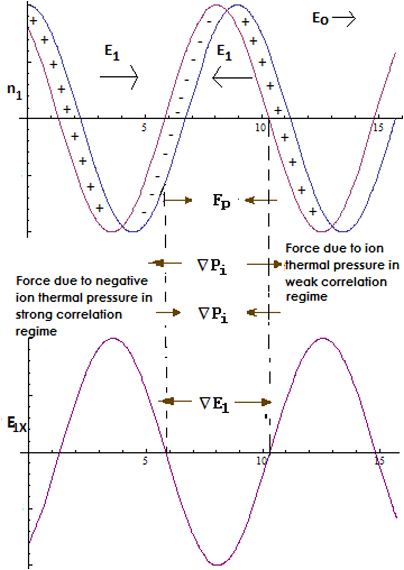
Fig. 1. Physical mechanism of OTSI in weakly and strongly coupled plasma.

Consider a laser pump $({\rm \omega} _0,\,\vec{k}_0)$ decays into two sideband waves (${\rm \omega} _{a,b},\vec{k}$) and one low frequency (${\rm \omega}, \,\vec{k}$) mode density perturbation where ${\rm \omega} _{a,b} = {\rm \omega} \mp {\rm \omega} _0$ and $\vec{k}_0\approx 0$. Here (${\rm \omega}, \,\vec{k}$) may not be an eigenmode of the system; it could be a driven mode. However, the sidebands are the Langmuir eigenmodes within a slight frequency mismatch due to nonlinear coupling. The dipole laser pump field is taken to be coherent given by $\vec{E}_0 = \hat{z}A_0e^{-i{\rm \omega} _0t}$ with ω₀ ≈ ω_pe. The electrostatic potentials are

(6)$${\rm \varphi} _l = Ae^{-i({\rm \omega} t-\vec{k}\cdot \vec{r})},$$

(7)$${\rm \varphi} _{a,b} = A_{a,b}e^{-i({\rm \omega} _{a,b}t-\vec{k}\cdot \vec{r})}.$$

The perturbed equation of motion for electron fluid is

(8)$$n_{e0}m_e\left( {\displaystyle{{\partial {\vec{v}}_{e1}} \over {\partial t}} + {\vec{v}}_{e1}\cdot \nabla {\vec{v}}_{e1}} \right) = -en_{e0}(\vec{E}_0-\nabla {\rm \varphi} )-\nabla P_{e1}.$$

The perturbed electron continuity equation is

(9)$$\displaystyle{{\partial n_{e1}} \over {\partial t}} + n_{e0}\nabla \cdot \vec{v}_{e1} + \nabla \cdot \left( {\displaystyle{1 \over 2}n_{e1}{\vec{v}}_{e1}} \right) = 0,$$

where $\vec{v}_{e1},P_{e1},n_{e1,}{\rm \varphi} $ are the perturbed electron velocity, pressure, density, and the electric potential, respectively, and n _e0 is the equilibrium electron density. Here the electrons will contribute to both, the high-frequency part and the low-frequency part. The high-frequency part corresponds to the laser (ω₀) and sidebands (ω_a,  ω_b) where electrons move independently of ions and the low-frequency part corresponds to the low-frequency mode (ω)where the electrons move along with ions in quasi-neutral manner. Hence for the electrons the quantities $\vec{v}_{e1},\,P_{e1},\,n_{e1},$ and φ each contains a high-frequency part ($\vec{v}_{e0}$, $\vec{v}_{ea,b},\,P_{ea,b},\,{\rm \varphi} _{a,b}$, and n _ea,b) and a low-frequency part ($\vec{v}_{el},\,P_{el},\,{\rm \varphi} _l$, and n _el).

To the lowest order of Eq. (8), the motion in response to high-frequency laser electric field E ₀ is

(10)$$\displaystyle{{\partial {\vec{v}}_{e0}} \over {\partial t}} = -\displaystyle{{e{\vec{E}}_0} \over {m_e}}$$

This gives the electron oscillatory velocity $\vec{v}_{e0} = \displaystyle{{e{\vec{E}}_0} \over {m_ei{\rm \omega} _0}}$.

For the high-frequency sidebands, the equation of motion for electron fluid is-

(11)$${m_e\displaystyle{{\partial {\vec{v}}_{ea,b}} \over {\partial t}} = e\nabla {\rm \varphi} _{a,b}-\displaystyle{{\nabla P_{ea,b}} \over {n_{e0}}}},$$

where $\vec{v}_{ea,b}$, n _ea,b, φ_a,b, and P _ea,b correspond to the high-frequency part at ${\rm \omega} _{a,b},\vec{k}$. The oscillatory velocities of electrons correspond to sideband waves (neglecting the pressure term) will be

(12)$$\vec{v}_{ea,b} = -\displaystyle{{e\vec{k}} \over {m_e{\rm \omega} _{a,b}}}{\rm \varphi} _{a.b}.$$

In the low-frequency part, the sidebands, and the pump wave beat and produce a low-frequency ponderomotive force $\vec{F}_p$ on electrons as ω = ω_a,b ± ω₀. Hence the equation of motion for low-frequency electrons along with the ponderomotive force is given by

(13)$$m_e\left( {\displaystyle{{\partial {\vec{v}}_{el}} \over {\partial t}} + {\vec{v}}_{e0}\cdot i\vec{k}{\vec{v}}_{ea} + \vec{v}_{e0}^{^\ast} \cdot i\vec{k}{\vec{v}}_{eb}} \right) = e\nabla {\rm \varphi} _l-\displaystyle{{i\vec{k}n_{el}T_e} \over {n_{e0}}},$$

where $\vec{v}_{el}$, n _el, and φ_l correspond to low-frequency part and T _e is the electron temperature. The ponderomotive force $\vec{F}_p$ can be defined as

(14)$$\vec{F}_p = e\nabla {\rm \varphi} _p = -({{m_e} / 2})\nabla (\vec{v}_{e0}\cdot \vec{v}_{ea} + \vec{v}^{^\ast}_{e0} \cdot \vec{v}_{eb}).$$

This gives the ponderomotive potential

(15)$${\rm \varphi} _p = \displaystyle{{\vec{k}\cdot {\vec{v}}_{e0}} \over {2{\rm \omega} _a}}{\rm \varphi} _a + \displaystyle{{\vec{k}\cdot {\vec{v}}^{^\ast}_{e0}} \over {2{\rm \omega} _b}}{\rm \varphi} _b.$$

Using Eqs. (14) and (15) in Eq. (13) we get

(16)$$m_e\displaystyle{{\partial {\vec{v}}_{el}} \over {\partial t}} = e\nabla \lpar {{\rm \varphi}_l + {\rm \varphi}_p} \rpar -\displaystyle{{i\vec{k}n_{el}T_e} \over {n_{e0}}}.$$

The low-frequency part of Eq. (9) gives

(17)$$\displaystyle{{\partial n_{el}} \over {\partial t}} + n_{e0}i\vec{k}\cdot \vec{v}_{el} = 0.$$

Using Eqs. (16) and (17) we can find the low-frequency electron density perturbation which is due to the ponderomotive and self-consistent potential φ_p and φ_l

(18)$$n_{el} = \displaystyle{{k^2} \over {4{\rm \pi} e}}{\rm \chi} _e({\rm \varphi} _l + {\rm \varphi} _p),$$

where χ _e is the low-frequency electron susceptibility at ω, k. For ω ≪ kv _th (v _th = (2T _e/m _e)^1/2 is electron thermal speed), ${\rm \chi} _e\approx {{2{\rm \omega} _{pe}^2} / {k^2v_{th}^2}} = {{{\rm \omega} _{pi}^2} / {k^2C_{s0}^2}} $ (where ω_pi = ((4πn _i0Z ²e ²)/m _i)^1/2is ion plasma frequency and C _S0 = (ZT _e/m _i)^1/2). The equation of motion of strongly coupled ion fluid is obtained by linearizing Eq. (1) as

(19)$$\matrix{\displaystyle{{\partial {\vec{v}}_{i1}\lpar {\vec{r},t} \rpar } \over {\partial t}} + \displaystyle{{\nabla P_{i1}(\vec{r},t)} \over {n_{i0}m_i}} + \displaystyle{{Ze\nabla {\rm \varphi} _l(\vec{r},t)} \over {m_i}} = \hfill \cr \quad \int_{-\infty} ^t {d{t}^{\prime}} \int {d{r}^{\prime}{\rm \eta} _i\lpar {\vec{r}-\vec{{r}^{\prime}},t-{t}^{\prime}} \rpar } {\vec{v}}_{i1}\lpar {\vec{{r}^{\prime}},{t}^{\prime}} \rpar \hfill}, $$

where $\vec{v}_{i1},P_{i1},{\rm \varphi} _l$ are the perturbed ion velocity, pressure and the electric potential, respectively, and n _i0 equilibrium ion density. The quantity η_i may be identified as a nonlocal viscoelastic operator (Berkovsky, Reference Berkovsky1992; Kaw and Sen, Reference Kaw and Sen1998) which accounts for memory effects and for the short-range order that begins to develop in the plasma as a result of the growing correlation between the ions with increasing values of Γ_i. If the memory function is regarded as a simple exponential function with τ_m as the relaxation time, then the Fourier transform of η_i can be expressed as (Kaw and Sen, Reference Kaw and Sen1998)

(20)$${\rm \eta} _i\lpar {{\rm \omega}, k} \rpar = \displaystyle{{{\rm \eta} k^2 + \left( {\displaystyle{{\rm \eta} \over 3} + {\rm \zeta}} \right)\vec{k}(\vec{k}\cdot )} \over {m_in_{i0}\lpar {1-i{\rm \omega} {\rm \tau}_m} \rpar }},$$

where ω and k are the frequency and the wave number of the low-frequency mode, η, ζ are shear and bulk viscosities. Combining Eqs. (19) and (20) we can express the GHD equation as

(21)$$\matrix{\left[ {{\rm 1} + {\rm \tau}_m\displaystyle{\partial \over {\partial t}}} \right]\left[ {m_{i}n_{i0}\displaystyle{{\partial {\vec{v}}_{i1}} \over {dt}} + Zen_{i0}\nabla {\rm \varphi}_l + \nabla P_{i1}} \right] \hfill \cr \quad = {\rm \eta} \nabla \cdot \nabla {\vec{v}}_{i1} + \left( {{\rm \zeta} + \displaystyle{{\rm \eta} \over 3}} \right)\nabla \lpar {\nabla \cdot {\vec{v}}_{i1}} \rpar. \hfill} $$

Linearizing the ion continuity equation given by Eq. (2)

(22)$$\displaystyle{{\partial n_{i1}} \over {\partial t}} + n_{i0}i\vec{k}\cdot \vec{v}_{i1} = 0.$$

The ion density perturbation n _i1 can be obtained by using Eq. (22) to eliminate the perturbed velocity in Eq. (21) which gives

(23)$$n_{i1} = -\displaystyle{{k^2} \over {4{\rm \pi} Ze}}{\rm \chi} _i{\rm \varphi} _l,$$

where χ _i is the ion susceptibility such that

(24)$${\rm \chi} _i = -\displaystyle{{{\rm \omega} _{\,pi}^2} \over {\left[ {{\rm \omega}^{\rm 2}-{\rm \gamma}_i{\rm \mu}_ik^{\rm 2}v_{thi}^2 + \displaystyle{{i{\rm \omega} {\rm \eta}^{^\ast}k^2a_i^2 {\rm \omega}_{\,pi}} \over {(1-i{\rm \omega} {\rm \tau}_m)}}} \right]}},$$

where γ _i = C _pi/C _vi is an adiabatic index, v _thi = (2T _i/m _i)^1/2 is the ion thermal velocity, ${\rm \mu} _i\lpar {{\rm \Gamma}_i} \rpar = \lpar {1/T_i} \rpar \lpar {\partial P_i/\partial n_i} \rpar _{T_i} = 1 + u({\rm \Gamma} _i)/3 \;+ \lpar {{\rm \Gamma}_i/9} \rpar \partial u({\rm \Gamma} _i)/\partial {\rm \Gamma} _i$ is compressibility (Ichimaru et al., Reference Ichimaru, Iyetomi and Tanaka1987) and u(Γ_i) is the normalized excess internal energy. For weakly coupled plasma (Γ_i <1), $u({\rm \Gamma} _i)\approx -\sqrt 3 /2\,\,{\rm \Gamma} _i^{3/2} $ and for 1 ≤ Γ_i ≤ 200, Slattery et al. (Reference Slattery, Doolen and DeWitt1980; Reference Slattery, Doolen and DeWitt1982) have given the empirical relation$u({\rm \Gamma} _i) = -0.89{\rm \Gamma} _i + 0.95{\rm \Gamma} _i^{1/4} + 0.19{\rm \Gamma} _i^{-1/4} -0.81$. For weak coupling (Γ_i ≈ 0) the value of μ _i = 1. As we increase Γ_i the value of μ _i decreases, goes to 0 for Γ_cr ≈ 3 and becomes negative for Γ_i >Γ_cr. Here τ_m and η* are given by

(25a)$${\rm \tau} _m = \displaystyle{{{\rm \eta} ^{^\ast}} \over {{\rm \omega} _{\,pi}{\rm \lambda} _i^2}} \displaystyle{{a_i^2} \over {1-{\rm \gamma} _i{\rm \mu} _i + \displaystyle{4 \over {15}}u({\rm \Gamma} _i)}}$$

(25b)$${\rm \eta} {^\ast} = \displaystyle{{\left( {\displaystyle{{4{\rm \eta}} \over 3} + {\rm \zeta}} \right)} \over {m_in_{i0}{\rm \omega} _{\,pi}a_i^2}} $$

where λ_i and a _i are the Debye length and mean interparticle distance for ions, respectively. The dependence of η* on Γ_i is more complicated and cannot be expressed in a simple closed form. Numerically calculated values using codes (Ichimaru et al., Reference Ichimaru, Iyetomi and Tanaka1987) show that it is of order unity (≈1.12) for values of Γ_i close to 1, goes to a minimum value (≈0.06) for Γ_i ≈ 10 and then monotonically increases for higher values of Γ_i.

Poisson's equation for the low-frequency part is given by

(26)$$k^2{\rm \varphi} _l = 4{\rm \pi} e\lpar {Zn_{i1}-n_{el}} \rpar .$$

Substituting the value of n _el and n _i1 from Eqs. (18) and (23) in Eq. (26) we get

(27)$${\rm \varepsilon} {\rm \varphi} _l = -{\rm \chi} _e{\rm \varphi} _p,$$

where ε = 1 + χ _i + χ _e.

Using Eq. (9), the continuity equation for sidebands is given by

(28)$$\displaystyle{{\partial n_{ea}} \over {\partial t}} + n_{e0}i\vec{k}\cdot \vec{v}_{ea} + i\vec{k}\cdot \left( {\displaystyle{1 \over 2}n_{el}{\vec{v}}^{^\ast}_{e0}} \right) = 0,$$

(29)$$\displaystyle{{\partial n_{eb}} \over {\partial t}} + n_{e0}i\vec{k}\cdot \vec{v}_{eb} + i\vec{k}\cdot \left( {\displaystyle{1 \over 2}n_{el}{\vec{v}}_{e0}} \right) = 0.$$

Using Eqs. (11), (28) and $({\rm \omega} _j,\vec{k})$ (29), the linear density perturbations at the sidebands are given by

(30)$$n_{ej}^L = \displaystyle{{k_{}^2} \over {4{\rm \pi} e}}{\rm \chi} _{ej}{\rm \varphi} _j,\quad j = a,b,$$

where χ _ej is the electron susceptibility at sideband. One may write ${\rm \chi} _{ej} = -({\rm \omega} _{pe}^2 + (3/2)k_{}^2 v_{th}^2 )/{\rm \omega} _j^2 $. The non-linear density perturbations at (${\rm \omega} _{a,b},\vec{k}$) due to the conjunction of density perturbation n _el with oscillatory velocity v _e0 from Eqs. (28) and (29) are

(31)$$n_{ea}^{NL} = \displaystyle{{\vec{k}\cdot {\vec{v}}^{^\ast}_{e0}} \over {2{\rm \omega} _a}}n_{el} = \displaystyle{{\vec{k}\cdot {\vec{v}}^{^\ast}_{e0}} \over {2{\rm \omega} _a}}\displaystyle{{k^2(1 + {\rm \chi} _i){\rm \chi} _e{\rm \varphi} _p} \over {4{\rm \pi} e{\rm \varepsilon}}}, $$

(32)$$n_{eb}^{NL} = \displaystyle{{\vec{k}\cdot {\vec{v}}_{e0}} \over {2{\rm \omega} _b}}n_{el} = \displaystyle{{\vec{k}\cdot {\vec{v}}_{e0}} \over {2{\rm \omega} _b}}\displaystyle{{k^2(1 + {\rm \chi} _i){\rm \chi} _e{\rm \varphi} _p} \over {4{\rm \pi} e{\rm \varepsilon}}}. $$

The Poisson's equation for high-frequency sidebands is

(33)$$k^2{\rm \varphi} _{a,b} = -4{\rm \pi} e\lpar {n_{ea,b}^L + n_{ea,b}^{NL}} \rpar .$$

Using Eqs. (30)–(32) in Eq. (33), we obtain

(34)$${\rm \varepsilon} _j{\rm \varphi} _j = {{-4{\rm \pi} en_{ej}^{NL}} / {k_{}^2}}, \quad j = a,b,$$

where ${\rm \varepsilon} _j = 1 + {\rm \chi} _{ej} = 1-({\rm \omega} _{pe}^2 + (3/2)k_{}^2 v_{th}^2 )/{\rm \omega} _j^2 $. Using Eqs. (27), (31) and (32) in Eq. (34) we get

(35)$${\rm \varphi} _a = \displaystyle{{\vec{k}\cdot {\vec{v}}^{^\ast}_{e0}} \over {2{\rm \omega} _a{\rm \varepsilon} _a}}\lpar {1 + {\rm \chi}_i} \rpar {\rm \varphi} _l,$$

(36)$${\rm \varphi} _b = \displaystyle{{\vec{k}\cdot {\vec{v}}_{e0}} \over {2{\rm \omega} _b{\rm \varepsilon} _b}}\lpar {1 + {\rm \chi}_i} \rpar {\rm \varphi} _l.$$

Using Eqs. (15), (35) and (36) in Eq. (27), we finally obtain the dispersion relation for OTSI as

(37)$${\rm \varepsilon} = -{\rm \chi} _e\lpar {1 + {\rm \chi}_i} \rpar \displaystyle{{{\vert {\vec{k}\cdot {\vec{v}}_{e0}} \vert } ^2} \over 4}\left( {\displaystyle{1 \over {{\rm \omega}_a^2 {\rm \varepsilon}_a}} + \displaystyle{1 \over {{\rm \omega}_b^2 {\rm \varepsilon}_b}}} \right).$$

Define a frequency mismatch ${\rm \Delta} = {\rm \omega} _0-\lpar {{\rm \omega}_{pe}^2 + (3/2)k^2v_{th}^2} \rpar ^{{1 / 2}}$ and substituting the value ε_a,b and ω_a,b in Eq. (37), we can write the dispersion relation as

(38)$${\rm \varepsilon} = -{\rm \chi} _e\lpar {1 + {\rm \chi}_i} \rpar \displaystyle{{{\vert {\vec{k}\cdot {\vec{v}}_{e0}} \vert } ^2} \over 4}\displaystyle{{\rm \Delta} \over {{\rm \omega} _0\lpar {{\rm \Delta}^2-{\rm \omega}^2} \rpar }}.$$

Now using Eq. (38) we will study OTSI in two limits that is, kinetic limit where ωτ _m > 1 and the hydrodynamic limit where ωτ _m < 1. Here ω represents the frequency of the ion or the low-frequency mode. We first consider the kinetic regime.

Kinetic regime

In this regime ωτ _m > 1, we can write χ _e and χ _i from Eq. (24) as follows

(39)$${{\rm \chi} _e} = {{\rm \omega} _{\,pi}^2 /k^2C_{s0}^2}, \,\,{{\rm \chi} _i = -\displaystyle{{{\rm \omega} _{\,pi}^2} \over {\left[ {{\rm \omega}^{\rm 2}-{\rm \gamma}_i{\rm \mu}_ik^{\rm 2}v_{thi}^2 -\displaystyle{{{\rm \eta}^{^\ast}{\rm \omega}_{\,pi}k^2a_i^2} \over {{\rm \tau}_m}}} \right]}}}$$

Using Eq. (25a) we can write Eq. (39) -

(40)$${\rm \chi} _i = -\displaystyle{{{\rm \omega} _{\,pi}^2} \over {\left[ {{\rm \omega}^{\rm 2}-(1 + \displaystyle{4 \over {15}}u({\rm \Gamma}_i))k^2v_{thi}^2} \right]}}$$

On substituting these values in Eq. (38) we get a biquadratic equation of ω

(41)$$\eqalign{& \lpar {{\rm \omega}^2-{\rm \Delta}^2} \rpar \left( {{\rm \omega}^2-\left( {1 + \displaystyle{4 \over {15}}u({\rm \Gamma}_i)} \right)k^2v_{thi}^2 -\displaystyle{{{\rm \omega}_{\,pi}^2} \over {\left( {1 + \displaystyle{{{\rm \omega}_{\,pi}^2} \over {k^2C_{s0}^2}}} \right)}}} \right) \cr & \quad = L\left( {{\rm \omega}^2-\left( {1 + \displaystyle{4 \over {15}}u({\rm \Gamma}_i)} \right)k^2v_{thi}^2 -{\rm \omega}_{\,pi}^2} \right){\rm \Delta},} $$

which can be simplified as

(42)$$\eqalign{& {\rm \omega} ^4-{\rm \omega} ^2\lpar {{\rm \omega}_{ac}^2 + {\rm \Delta}^2 + L{\rm \Delta}} \rpar + L{\rm \Delta} \left( {{\rm \omega}_{\,pi}^2 + \left( {1 + \displaystyle{4 \over {15}}u({\rm \Gamma}_i)} \right)k^2v_{thi}^2} \right) \cr & \quad + {\rm \Delta} ^2{\rm \omega} _{ac}^2 = 0,} $$

where

$$\eqalign{& \cr L = \displaystyle{{{\vert {v_{e0}} \vert } ^2} \over {4C_{s0}^2}} \displaystyle{{{{{\rm \omega} _{\,pi}^2} / {{\rm \omega} _0}}} \over {\left( {1 + \displaystyle{{{\rm \omega}_{\,pi}^2} \over {k^2C_{s0}^2}}} \right)}}\quad {\rm and} \cr \quad {\rm \omega} _{ac}^2 = \left( {1 + \displaystyle{4 \over {15}}u({\rm \Gamma}_i)} \right)k^2v_{thi}^2 + \displaystyle{{{\rm \omega} _{\,pi}^2} \over {\left( {1 + \displaystyle{{{\rm \omega}_{\,pi}^2} \over {k^2C_{s0}^2}}} \right)}},} $$

if we normalized ω by ω_pi Eq. (42) will be

(43)$$\eqalign{& {{{\rm \omega}} ^{\prime 4}}-{\rm \omega} ^{\prime 2}\lpar {{{\rm \omega}}_{ac}^{\prime 2} + {{{\rm \Delta}}^{\prime 2}} + {L}^{\prime}{{\rm \Delta}}^{\prime}} \rpar \cr & \quad + {L}^{\prime}{{\rm \Delta}} ^{\prime} \left( {1 + \left( {1 + \displaystyle{4 \over {15}}u({\rm \Gamma}_i)} \right)\displaystyle{{T_i} \over {ZT_e}}k^2{\rm \lambda}_e^2} \right) + {{{\rm \Delta}} ^{\prime 2}}{{\rm \omega}}_{ac}^{\prime 2} = 0,} $$

where

$${{\rm \omega}} ^{\prime} = \displaystyle{{\rm \omega} \over {{\rm \omega} _{\,pi}}},$$

$${\rm \omega} _{ac}^{\prime 2} = \left( {1 + \displaystyle{4 \over {15}}u({\rm \Gamma}_i)} \right)\displaystyle{{T_i} \over {ZT_e}}k^2{\rm \lambda} _e^2 + \displaystyle{1 \over {\left( {1 + \displaystyle{1 \over {k^2{\rm \lambda}_e^2}}} \right)}},$$

$${L}^{\prime} = \displaystyle{{{\vert {v_{e0}} \vert } ^2} \over {4C_{s0}^2}} \displaystyle{{{{{\rm \omega} _{\,pi}} / {{\rm \omega} _0}}} \over {\left( {1 + \displaystyle{1 \over {k^2{\rm \lambda}_e^2}}} \right)}},$$

$${{\rm \Delta}} ^{\prime} = \displaystyle{{\rm \Delta} \over {{\rm \omega} _{\,pi}}} = \displaystyle{{{\rm \omega} _0} \over {{\rm \omega} _{\,pi}^{}}} -\left( {\displaystyle{{{\rm \omega}_{\,pe}^2} \over {{\rm \omega}_{\,pi}^2}} + \displaystyle{{m_i} \over {Zm_e}}\displaystyle{3 \over 2}k^2{\rm \lambda}_e^2} \right)^{{1 / 2}}.$$

The two roots of Equation (43) are

(44)$$\eqalign{& \omega ^{{\prime 2}} = \displaystyle{1 \over 2} \bigg[ (\omega _{ac}^{{\prime 2}} + \Delta ^{{\prime 2}} + L^{\prime}\Delta ^{\prime}) - \sqrt{\lpar \omega _{ac}^{{\prime 2}} + \Delta^{{\prime 2}} + L^{\prime}\Delta ^{\prime} \rpar^{2} -4 {\left( {L^{\prime}\Delta ^{\prime}\left( {1 + \left( {1 + \displaystyle{4 \over {15}}u(\Gamma _i)} \right)\displaystyle{{T_i} \over {ZT_e}}k^2\lambda _e^2 } \right) + \Delta ^{{\prime 2}}\omega _{ac}^{{\prime 2}} } \right)}} \bigg]}.$$

Instability occurs when Δ^′ <0 and

$$\vert {{{\rm \Delta}}^{\prime}} \vert \lt \displaystyle{{{L}^{\prime}\left( {1 + \left( {1 + \displaystyle{4 \over {15}}u({\rm \Gamma}_i)} \right)\displaystyle{{T_i} \over {ZT_e}}k^2{\rm \lambda}_e^2} \right)} \over {{{\rm \omega}}_{ac}^{\prime 2}}}. $$

If the two conditions given above are satisfied then the value of ω^′2 will be negative which gives two imaginary roots, out of which one grows with time. This root corresponds to OTSI. Thus the growth rate of OTSI in the kinetic regime is

(45)$$\displaystyle{{\rm \gamma} \over {{\rm \omega} _{\,pi}}} = \left[ {\displaystyle{1 \over 2}\left\{ \matrix{({{\rm \omega}}_{ac}^{\prime 2} + {{{\rm \Delta}}^{\prime 2}} + {L}^{\prime}{{\rm \Delta}}^{\prime})- \sqrt {{\lpar {{{\rm \omega}}_{ac}^{\prime 2} + {{{\rm \Delta}}^{\prime 2}} + {L}^{\prime}{{\rm \Delta}}^{\prime}} \rpar }^2- 4\left( {{L}^{\prime}{{\rm \Delta}}^{\prime}(1 + \left( {1 + \displaystyle{4 \over {15}}u({\rm \Gamma}_i)} \right)\displaystyle{{T_i} \over {ZT_e}}k^2{\rm \lambda}_e^2 ) + {{{\rm \Delta}}^{\prime 2}}{{\rm \omega}}_{ac}^{\prime 2}} \right) }} \right\}} \right]^{1/2}.$$

In the limit Γ_i → 0 the growth rate in Eq. (45) reduces to the standard growth rate of OTSI (Ramachandran and Tripathi, Reference Ramachandran and Tripathi1997). In Figure 2, we have plotted the growth rate (γ) as a function of k for Γ_i ≈ 0 (for the weak coupling limit) and for Γ_i = 2.5 and 5. The parameters which we have used in Figure 2 are as follows. Since OTSI takes place near the critical density (n _cr) region where ω₀ ≈ ω_pe, we take n _i ≈10²¹ cm⁻³ (n _e ≈ n _cr ≈ 10²² cm⁻³ for laser 351 nm), T _e ≈ 100 − 150 eV, T _i ≈ 45 − 100 eV, laser intensity(I) is10¹⁴W/cm² and Z = 5 − 10 for Al ion plasma.

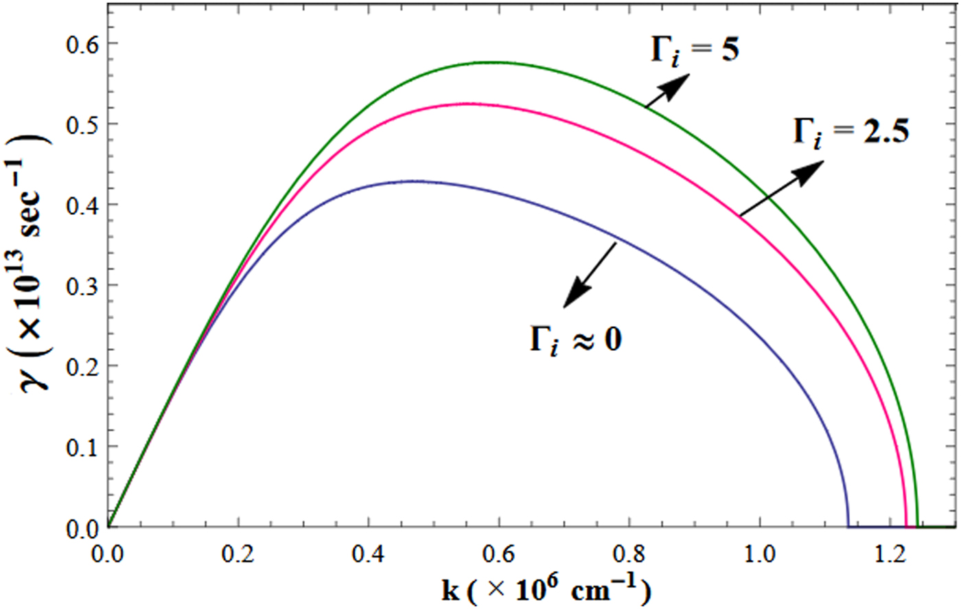
Fig. 2. Variation in growth rate (γ) as a function of k for Γ_i = 2.5 and Γ_i = 5 in the kinetic regime. The case of Γ_i ≈ 0 is included for comparison with weak coupling limit (Γ_i <1).

In the plot, we can see the growth rate increases with Γ_i. For example at k ≈ 0.6 × 10⁶ cm⁻¹, the enhancement in the growth rate for Γ_i = 2.5 is about 25% and for Γ_i = 5 is about 40%. In Figure 3, we plot the growth rate (γ) as a function of normalized pump frequency (ω₀/ω_pe) for k = 0.5 × 10⁶ cm⁻¹ with different Γ_i ≈ 0, 2.5 and 5. OTSI will occur only when ω₀ ≈ ω_pe. For higher values of ω₀, at which Δ^′ becomes positive, OTSI will vanish. Next, we give a posterior justification for the kinetic regime condition γτ _m >1. For particular values of plasma parameters ω_pi, λ_i and ion coupling parameter Γ_i, τ_m can be obtained from Eq. (25a). So in Fig. 2 for Γ_i = 2.5, τ_m ≈ 1.8 × 10⁻¹¹ s while the typical growth rate γ ≈ 0.45 × 10¹³ s⁻¹ and hence γτ _m ≈ 80. Similarly for Γ_i = 5, τ_m ≈ 2.7 × 10⁻¹² s and γτ _m ≈ 15. Thus in Figure 2 and Figure 3, OTSI is indeed in the kinetic regime for Γ_i = 2.5 as well as for Γ_i = 5. It should be noted that since γ → 0 as k → 0, the growth rate must be chosen sufficiently away from zero for the kinetic regime to be valid.

Fig. 3. Variation in growth rate (γ) as a function of ω₀/ω_pe for k = 0.5 × 10⁶ cm⁻¹ with different values of Γ_i in the kinetic regime. The case of Γ_i ≈ 0 is included for comparison with weak coupling limit (Γ_i <1).

Hydrodynamic regime

In this regime where ωτ _m <1, χ _e and χ _i from Eq. (24) will be as follows

(46)$${{\rm \chi} _e} = {{\rm \omega} _{\,pi}^2 /k^2C_{s0}^2}, \ldots {\rm \chi} _i = -\displaystyle{{{\rm \omega} _{\,pi}^2} \over {\lsqb {{\rm \omega}^{\rm 2}-{\rm \gamma}_i{\rm \mu}_ik^{\rm 2}v_{thi}^2} \rsqb }}.$$

On substituting these values in Eq. (38), the biquadratic equation which we obtain is

(47)$$\eqalign{& {{{\rm \omega}} ^{\prime 4}}-{{{\rm \omega}} ^{\prime 2}}\lpar {{{\rm \omega}}_{ac}^{\prime 2} + {{{\rm \Delta}}^{\prime 2}} + {L}^{\prime}{{\rm \Delta}}^{\prime}} \rpar + {L}^{\prime}{{\rm \Delta}} ^{\prime} \cr & \quad \left( {1 + {\rm \gamma}_i{\rm \mu}_i\displaystyle{{T_i} \over {ZT_e}}k^2{\rm \lambda}_e^2} \right) + {{{\rm \Delta}} ^{\prime 2}}{{\rm \omega}} _{ac}^{\prime 2} = 0,} $$

where

$${{\rm \omega}} ^{\prime} = \displaystyle{{\rm \omega} \over {{\rm \omega} _{\,pi}}},$$

$${{\rm \omega}} _{ac}^{\prime 2} = {\rm \gamma} _i{\rm \mu} _i\displaystyle{{T_i} \over {ZT_e}}k^2{\rm \lambda} _e^2 + \displaystyle{1 \over {\left( {1 + \displaystyle{1 \over {k^2{\rm \lambda}_e^2}}} \right)}},$$

$${L}^{\prime} = \displaystyle{{{\vert {v_{e0}} \vert } ^2} \over {4C_{s0}^2}} \displaystyle{{{{{\rm \omega} _{\,pi}} / {{\rm \omega} _0}}} \over {\left( {1 + \displaystyle{1 \over {k^2{\rm \lambda}_e^2}}} \right)}},$$

$${{\rm \Delta}} ^{\prime} = \displaystyle{{\rm \Delta} \over {{\rm \omega} _{\,pi}}} = \displaystyle{{{\rm \omega} _0} \over {{\rm \omega} _{\,pi}^{}}} -\left( {\displaystyle{{{\rm \omega}_{\,pe}^2} \over {{\rm \omega}_{\,pi}^2}} + \displaystyle{{m_i} \over {Zm_e}}\displaystyle{3 \over 2}k^2{\rm \lambda}_e^2} \right)^{{1 / 2}}.$$

Two roots of Eq. (47) are-

(48)$$\eqalign{&{\omega }^{\prime 2} = \displaystyle{1 \over 2}\Bigg[ ({\omega }^{\prime 2}_{ac} + {{\Delta }^{\prime 2}} + {L}^{\prime}{\Delta }^{\prime}) -\sqrt {\matrix{\left( {\omega }^{\prime 2}_{ac} + {\Delta }^{\prime 2} + {L}^{\prime}{\Delta }^{\prime} \right)^2 -4\left( {L}^{\prime}{\Delta }^{\prime}\left( 1 + \gamma _i\mu _i\displaystyle{{T_i} \over {ZT_e}}k^2\lambda _e^2 \right) + {\Delta }^{\prime 2}{\omega }^{\prime 2}_{ac} \right)}} \Bigg].}$$

For instability Δ^′ must be negative and

$$\vert {{{\rm \Delta}}^{\prime}} \vert \lt \displaystyle{{{L}^{\prime}\left( {1 + {\rm \gamma}_i{\rm \mu}_i\displaystyle{{T_i} \over {ZT_e}}k^2{\rm \lambda}_e^2} \right)} \over {{{\rm \omega}} _{ac}^{\prime 2}}}. $$

For the above two conditions, the value of ω^′2 will be negative which further gives two imaginary roots and hence one of the roots of Eq. (48) gives the growth rate of OTSI in the hydrodynamic regime such that

(49)$$\displaystyle{\gamma \over {\omega _{\,pi}}} = \left[ {\displaystyle{1 \over 2} \left\{(\omega _{ac}^{{\prime}2} + \Delta ^{{\prime}2} + L^{\prime}\Delta ^{\prime})- \sqrt{ \matrix{\left( {\omega _{ac}^{{\prime}2} + \Delta ^{{\prime}2} + L^{\prime}\Delta ^{\prime}} \right)^2- 4\left( {L^{\prime}\Delta ^{\prime}(1 + \left( {1 + \gamma _i\mu _i\displaystyle{{T_i} \over {ZT_e}}k^2\lambda _e^2 } \right) + \Delta ^{{\prime}2}\omega _{ac}^{{\prime}2} } \right) \hfill} \hfill} } \right\} \right]^{1/2}.$$

The growth rate in Eq. (49) reduces to the standard growth rate of OTSI in the limit Γ_i → 0. In Figure 4 we have plotted the growth rate (γ) as a function of k for Γ_i = 9 and Γ_i = 14, where the laser intensity (I) is 10¹⁴W/cm², n _e ≈ 10²² cm⁻³, T _e ≈ 75 eV, T _i = 20 − 25 eV, Z = 10–11 (for Al ion) and ω₀ ≈ ω_pe. The curve Γ_i ≈ 0 shows the growth rate in weakly coupled plasma.

Fig. 4. Variation in growth rate (γ) as a function of k for Γ_i = 9 and Γ_i = 14 in the hydrodynamic regime. The case of Γ_i ≈ 0 is included for comparison with weak coupling limit (Γ_i <1).

The plot shows a large increment in the growth rate of OTSI (by almost 200%) for k = 1 × 10⁶cm⁻¹ and Γ_i = 14. For Γ_i = 9 the enhancement in the growth rate at k = 1 × 10⁶ cm⁻¹ is about 160%. Thus the destabilization effect of strongly coupled ions is much severe in the hydrodynamic limit than in the kinetic limit. To give a posterior justification for the hydrodynamic regime condition γτ _m <1, we find for Γ_i = 9, τ_m ≈ 0.3 × 10⁻¹³ s while the typical growth rate γ ≈ 0.6 × 10¹³ s⁻¹ and hence γτ _m ≈ 0.1, similarly for Γ_i = 14, τ_m ≈ 0.9 × 10⁻¹⁴ s and γτ _m ≈ 0.06. Hence in Figure 4, OTSI is in the hydrodynamic regime for Γ_i = 9 as well as for Γ_i = 14.

Summary and discussions

In this paper, we have studied the OTSI in the presence of strongly coupled ions. The situation involving strongly coupled ions is likely to arise in a number of cases. For example in the case of Au blow of plasma near the hohlraum wall in the indirect drive experiments in ICF scheme, the gold ions may become strongly coupled due to large electronic charge. In case of the direct drive approach, the carbon ions of the ablator material in the coronal plasma may become strongly coupled. Similarly, in the case of laser-driven ion accelerator, a pre-plasma of C or Al ions is formed on the target's front side, where the density of plasma is near critical density. In this region, C or Al ions may become strongly coupled. Typically in these situations, the ion correlation factor Γ_i can be as high as 2–15. In this regime, the ion behaves as strongly coupled viscoelastic fluid. The strong coupling effects are included here via GHD equation. It is shown that in a typical parameter regime of OTSI, these strong correlation effects modify the compressibility μ _i(Γ_i). This can be integrated once to give the ion pressure P _i as a function of Γ_i given by the expression $P_i = (0.73-0.3{\rm \Gamma} _i + 0.31{\rm \Gamma} _i^{1/4} + 0.07{\rm \Gamma} _i^{-1/4} )n_iT_i.$ As can be seen from this expression with increasing Γ_i ion pressure decreases and for Γ_i >4 it becomes negative. We have examined the effects of strong correlation in the two regimes that is, the kinetic regime (valid for ωτ _m >1) and the hydrodynamic regime (valid for ωτ _m <1). Our results show that these strong correlation effects lead to significant enhancement of the growth rate of OTSI. This destabilization is caused by enhancing bunching of ions due to its negative pressure as shown in Figure 1.

It should be noted that extreme compression also leads to plasma electrons and ions correlation. Strong correlations generated due to high compression cannot be described by GHD theory (Avinash, Reference Avinash2015). These effects may also become significant in laser fusion targets and ion acceleration which will be the subject of future publication.