NOMENCLATURE
- API
Application Programming Interface
- CFD
Computational Fluid Dynamics
- CSD
Computational Structural Dynamics
- CSGE
Control System Graphical Editor
- DYW
Dynamic Wake Model
- FAA
Federal Aviation Agency
- FLME
FLIGHTLAB Model Editor
- GPU
Graphical Processing Unit
- GUI
Graphical User Interface
- HAG
Height Above Ground
- Hstab
Horizontal Stabilator
- N-S CFD
Navier Stokes Computational Fluid Dynamics
- SAS
Stability Augmentation System
- SIMQT
Simulator Qualification Test
- VE
Virtual Engineering
- VPLAB
Virtual Pilot Laboratory
- VPM
Vortex Particle Method
- Cp
coefficient of power
- CT
coefficient of thrust
- CQ
coefficient of torque
- Deg
degrees
- FSCG
fuselage station centre of gravity
- Ft
feet
- G.W.
gross weight
- Hp
horse power
- In
inches
- Kn
knots
- lb
pounds
- Mu
advance ratio
- Pres. Alt.
pressure altitude
- R
rotor radius
- Rad
radians
- RPM
revolutions per minute
- Sec
second
- Rad/Sec
radians/second (units of damping)
- Whl. Ht.
wheel Height
- X
longitudinal position from rotor hub (positive aft)
- Y
lateral position from rotor hub (positive up)
- Z
vertical offset from rotor (positive right)
- αf
angle-of-attack of fuselage
Acronyms
Notation
1.0 INTRODUCTION
Faster computer processing capabilities, the use of modern computer science methodologies, and advances in physics-based modelling and simulation techniques have enabled the development of VE software tools to effectively support inter-disciplinary engineering applications. These tools are beginning to be used to support all aspects of the aircraft life cycle including acquisition, design, manufacturing, operations, testing and evaluation, and training. The following state-of-the-art features facilitate modelling and simulation in the software that have incorporated them.
(1) The use of an interpretive programming language
The ability to bypass compilation and both edit and execute a program interactively expedites the efficiency of software development and troubleshooting.
(2) Interactive access to essential mathematical operations for vector and matrix manipulation
Programming an equation in vector/matrix format, as the equation would appear in a textbook, as opposed to embedding multiple scalar equations in nested loops, expedites the programming of high-order equations.
(3) Object-oriented programming applications
Applications of object-oriented features greatly simplifies the structure and re-configurability of the software. For example, the use of method calls can automatically sequence and invoke a subset of software in all modelling components that are programmed to respond to that method call. The propagation of motion and forces throughout the model are each invoked with an associated method call.
(4) A library of generic modelling components
The ability to build a complex model from simpler reconfigurable building blocks with parameters that can be assigned interactively by the developer both expedites the development and reduces human error due to the use of predefined components that have been tested extensively in a variety of modelling applications.
(5) State-of-the-art physics-based modelling of rotorcraft phenomena
The modelling component library should be continually updated to reflect the latest advances in multidisciplinary modelling of rotorcraft, including aerodynamics, structures, propulsion, and control.
(6) A library of analysis utilities
Similar to the use of modelling components, standard analyses utilities can be programmed generically so that application-specific-parameters can be assigned interactively by the analyst.
(7) Arbitrary architecture modelling
In order to be useful, a VE modelling tool must have the capability to interconnect the modelling components into an arbitrary architecture. If the architecture were fixed, the VE tool developer could derive an explicit formulation for the solution of the coupled component equations but, since the component architecture is not fixed, an explicit solution formulation cannot be used. An iterative, numerical technique, however, can solve the resulting coupled multibody and multiple body dynamics equations implicitly, thereby eliminating the need for derivations of the coupled equations by the developer, again reducing the possibility of human error.
(8) Selective Fidelity Modelling
Different VE tasks require different levels of modelling sophistication. In order to make the most effective use of computational resources, varying levels of modelling sophistication for rotorcraft phenomena should be available. For example, the rotor wake may be modelled using finite state dynamic wake or vortex wake methods; structures may be modelled as rigid or elastic; and aerodynamic loads may be modelled as quasi-steady or unsteady.
(9) Graphical User Interfaces
In addition to being able to develop a model and run a simulation using the model by developing a program in the interpretive language, Graphical User Interfaces (GUIs) can be used to build models and perform analyses by providing the developer with modelling and analysis options and allowing the assignment of application-specific data. The GUIs then automatically generate the required program from the information provided by the developer. This can significantly reduce, or eliminate, the need for programming and thereby speed the development and reduce, or eliminate, human error.
(10) Open Architecture
The ability to allow the developer to expand on the component library and the analysis utilities is essential to addressing modelling and analysis issues not covered in the current software release.
(11) Interface to external programs
VE tools should include the capability to interface with external comprehensive modelling tools that complement the modelling domain of the VE tool, such as CFD and aeroacoustic modelling tools
FLIGHTLAB is a VE software tool, which is widely used in rotorcraft design, analysis, and full flight simulation applications, that incorporates all of the above features. The software supports the development of aircraft models, both fixed and rotary wing, with an extensive library of modelling components which have been used and validated in numerous, real-world applications. It has been continuously enhanced since its introduction in 1990 and used to develop a variety of high-fidelity rotary and fixed-wing aircraft configurations to support all phases of the product life-cycle, for both engineering analysis and real-time flight simulation. The tools have had the benefit of over 30 years of research and development and are continuously enhanced and updated with new features and capabilities. The following is a brief summary of the FLIGHTLAB VE tools. For a more extensive description, see Appendix A.
Development System: This is an interactive modelling and simulation environment to describe the flight vehicle and analyse its aeromechanics using a library of modelling components and engineering analysis utilities. Models can be developed by invoking and interconnecting modelling components in arbitrary architectures using a scripting language, or GUIs may be employed to facilitate modelling and analysis from pre-defined scripting templates.
PilotStation: The PilotStation software provides a desktop simulator for the Development Model as executed in the Development System. It includes an out-the-Window display, an instrument display, and a joystick interface. An interactive operator console display is also provided.
Run-Time System: The Run-Time System is a run-time environment for execution of real-time aeromechanics models. It includes the model driver, a command interface for executing the model, Application Programming Interface (API) and communication utilities to facilitate integration with other simulator systems in a distributed local area network, and a GUI for testing and troubleshooting.
Simulation Qualification Tool (SIMQT): This software tool automatically performs a set of simulated flight tests on an aeromechanics model and compares the results with reference data obtained from flight testing. The model and test results are plotted and tolerance bands for acceptance testing are displayed.
Viscous Vortex Particle Method (VPM): VPM provides interactional aerodynamics modelling of the mutual interference effect of all aerodynamic components on the flow field.
The Virtual Pilot Laboratory (VPLAB): VPLAB provides a set of utilities for generating control histories that drive the models though prescribed manoeuvres and flightpath waypoints.
The Run-Time System and Simulation Qualification Test tools were initially developed to support integration and testing of models with simulators utilising a wide variety of simulation hardware, including visual display systems, image generators, control loaders, motion platforms, avionics systems and Instructor/Operator Stations. Objective testing of aeromechanics models against test data and subjective testing with experienced pilots have been part and parcel of this development experience.
This paper presents a description of these rotorcraft VE tools and their validation, and draws on a number of examples to illustrate their range of applications. Extensive validation of models against test data has taken place by FLIGHTLAB users over a long period and this paper discusses only examples of this work. Readers can refer to a wide range of publications by FLIGHTLAB users for more validations that have been performed.
The authors are conscious that their paper is essentially a description of the technical content and range of applications of a commercially available VE tool and they have striven to be impartial in the presentation of results. The history of FLIGHTLAB development has been a substantial technical experience involving a large number of users and it is intended that this publication brings this experience to a broader readership concerned with rotorcraft VE.
2.0 FLIGHTLAB – AIR VEHICLE MODELLING AND SIMULATION SOFTWARE
Advances in physics-based modelling and simulation techniques have enabled rotorcraft modelling and analysis tools to support new design and engineering applications such as coupled Computational Fluid Dynamics (CFD)/Computational Structural Dynamics (CSD) analysis and detailed rotor/body aerodynamic interaction analysis. Figure 1 shows the range of modelling capabilities provided by FLIGHTLAB.

Figure 1. FLIGHTLAB rotorcraft modelling and analysis capability.
The following is a brief summary of the capabilities identified in Fig. 1.
2.1 Multi-body dynamics
This refers to the ability to construct a model by arbitrarily interconnecting modelling elements, each with their own degrees of freedom, and using iterative numerical methods to solve the resulting fully coupled dynamic system. This has the advantage of eliminating the derivation and programming of the fully coupled equations, thereby reducing model development time and eliminating the potential for human error. While the iterative solution method is less computationally efficient than the explicit formulation that could be achieved with a manual derivation, the speed of modern computers has largely eliminated this disadvantage.
2.2 Blade element and finite element methodologies
Using a blade element model, detailed rotor aerodynamics and blade- and hub-retention dynamics can be accurately modelled. The blade element model is computationally efficient and has been extensively used for flight dynamics and handling qualities analysis as well as full rotorcraft flight simulation(Reference He, Goericke and Lee1,Reference He, Goericke and Kang2) . The finite element method significantly improves the rotor structural dynamics modelling by considering the nonlinear blade elasticity, which is important for vibratory loads prediction(Reference Saberi, Jung and Anastassiades3).
2.3 Unsteady airloads
Both blade element and finite element models are integrated with unsteady aerodynamics models, including dynamic stall for detailed blade section airloads evaluation(Reference He and Du Val4). In addition, modules are provided for blade element ducted fan modelling that include the effect of fan/duct interaction(Reference He and Xin5).
2.4 Viscous vortex particle method
The viscous VPM is a first-principle-based rotor/wing wake dynamics solution. It provides an accurate and computationally efficient method for complicated and/or novel rotor/wing wake and interference modelling(Reference He and Zhao6-Reference He and Rajmohan11). VPM currently does not run in real time and is used in an offline mode.
2.5 Interface to computational fluid dynamics codes
In recent years, first-principle-based rotorcraft aerodynamics methods (i.e. Navier-Stokes-based CFD airloads solvers) have been interfaced with FLIGHTLAB to offer a coupled CFD/CSD solution(Reference Rajmohan, Zhao and He8).
2.6 Flight and engine controls
To support full-flight rotorcraft modelling, modules are provided (such as gains, integrators, switches, transfer functions, etc.) to simulate flight control systems, ranging from simple mechanical controls with a Stability Augmentation System (SAS) to full digital fly-by-wire/light systems with integrated primary and automatic flight control systems.
2.7 Engines and drivetrain
Modules are provided for the modelling of the power turbine and gas generator with the applied turbine and gas generator torques obtained from thermodynamic tables as a function of rotational speed and fuel flow. Options for both quasi-static and dynamic modelling of the thermodynamics are provided. Modelling of the rotational speed degree of freedom of the power turbine and gas generator includes their inertia, the torque output of the thermodynamic tables, and the reaction torque of the rotors, as applied through the drivetrain. Control modules (such as gains, switches, math elements, transfer functions, etc.) are also provided for modelling engine fuel control and fuel dynamics. The drivetrain model includes the transmission, clutch, main rotor shaft, and tail rotor shaft.
Additional modules provide modelling capabilities of landing gears, fuel system, internal and external cargo, and more. The research reported in the references has underpinned the developments illustrated in Fig. 1.
3.0 VALIDATION
3.1 Overview
The FLIGHTLAB Development System has been used by a variety of organisations to simulate and analyse the behaviour of a wide range of existing aircraft and to support the design and testing of new and unique aircraft configurations. The unique configurations include tail sitters, tiltrotors, compound rotorcraft, coaxial rotorcraft, autogyros, and distributed propulsion aircraft. A selective fidelity modelling capability allows for reduction in the computational intensity by reducing the modelling sophistication for phenomena that are of secondary importance to the application. For example, rigid body structural modelling may be used in real-time training applications where structural loads are not being directly investigated. Validation is an essential activity to ensure the modelling fidelity is sufficient to support the required application. The level of modelling typically used for performance and handling qualities analysis includes blade element rotors with finite state dynamic inflow modelling of both the inflow at the rotor and for downwash interference effects on the fuselage and empennage(Reference He, Goericke and Kang2,Reference He and Du Val4,Reference Strope, Borden and Harding12) . Structural modelling of the rotor for these applications uses either rigid body, modal elastic or finite element representations(Reference Saberi, Jung and Anastassiades3). For detailed design and analysis, the flow field is modelled using VPM to capture the interactional aerodynamics of all vorticity producing elements(Reference He and Zhao6-Reference He and Rajmohan11). Interfacing to CFD codes provides high-fidelity modelling of the airloads(Reference Rajmohan, Zhao and He8). For structural loads analysis, finite element modelling of the rotor is used and a modal representation of the fuselage, obtained from a NASTRAN model, is used to couple the modal fuselage response with a full finite element NASTRAN model of the fuselage. Table 1 provides examples of the selective fidelity modelling options typically used for various modelling and simulation applications.
Table 1 Examples of selective fidelity modelling options applied to achieve required fidelity for different applications

The following sections discuss these validation efforts, including example plots comparing simulation and test data. The discussion also addresses the modelling and simulation challenges in each area and the model enhancements that were required to achieve an acceptable level of correlation with the test data.
3.2 Performance
Performance prediction is a basic necessity for any modelling and simulation tool. It requires trimming the model at a range of flight conditions and aircraft configurations and recording control settings, engine power, rotor thrust and torque, and other essential parameters. The software uses an iterative gradient approach to trim that can be carried out to any desired level of accuracy. The trim process can be difficult at the edge of the flight envelope due to discontinuities in the aerodynamics. The trim process has been enhanced to address this problem and provides a robust trim across the flight envelope. A detailed study of the ability of FLIGHTLAB models to accurately predict rotorcraft performance was conducted and reported in Reference He, Goericke and KangRef. 2. A number of modelling enhancements were made during this study to improve the performance prediction. Enhancements include modification to the inflow modelling, the addition of stall delay, the addition of wake decay, and modelling of rotor interference effects on the empennage. These enhancements and the associated validation effort are described in Reference He, Goericke and KangRef. 2 and summarised below.
Prediction of the power required for performance estimates is affected by inflow modelling accuracy, particularly at hover and low-speed flight conditions. The Peters and He finite state dynamic wake model, described in Reference Peters and HeRef. 13, is used for induced velocity modelling for performance predictions. The finite-state dynamic wake model uses a mathematical series representation of both radial and azimuthal inflow variation. Comparisons against test data were performed for two different orders of the dynamic wake series approximation; 3 states and 15 states. Increasing the order of the series approximation affects the power estimation accuracy as shown in Fig. 2(Reference He, Goericke and Kang2). This figure plots power coefficient (CP) vs. thrust coefficient (CT) for a UH-60 helicopter in ground effect and overlays test data with both a 3-state and a 15-state dynamic wake model. The dynamic wake model includes ground effect using a three-dimensional potential source.

Figure 2. Effect of inflow model order on hover performance(Reference He, Goericke and Kang2) Pres. Alt (ft): 3111 Whl. Ht. (ft. AGL): 5.0 F.S.C.G. (in): 347.1.
The rotor blade planform and twist for this vehicle were distributed toward an optimum inflow distribution for good hover performance. The blade element model used for analysis accurately represents the detailed blade platform and twist and therefore, it gives reasonably good prediction even with a 3-state wake model. But the 3-state model prediction does deviate from the measured data at higher lifting conditions due to the increasingly nonuniform variation of the induced inflow. That is why the higher-order finite state wake model (15 states) improved the results at the higher thrust region. While a 6-state model was not tested in this study, it may provide a good compromise between the 3- and 15-state results and it is still very computationally efficient.
In forward flight, the retreating blades experience reversed flow, which increases with speed and is the primary cause of stall encountered by the inboard blade sections, as discussed in Reference He, Goericke and KangRef. 2. The flow stall causes a large increase of rotor profile drag and hence, the power. But, the 3D flow due to rotor rotation can delay the blade stall and therefore, modelling the stall delay effect helps improve the prediction. This phenomena is also referred to as dynamic stall.
The stall delay model was developed analytically using a laminar 3D boundary-layer solution on a rotating wing(Reference Banks and Gadd14) and the model introduces the delay in terms of both maximum lift angle-of-attack and the angle-of-attack corresponding to the drag divergence in stall. Enhancing the blade element with the 3D stall delay model helps improve the prediction. This effect is further addressed in Reference He, Goericke and KangRef. 2.
3.3 Stability
Stability validation includes tests for longitudinal static stability and lateral directional static stability. Longitudinal static stability requires varying the airspeed about a trim point and recording the attitudes and control settings required to achieve the specified airspeed. Lateral directional stability requires varying the sideslip about a trim point and recording the attitudes and control settings required to achieve the specified sideslip. The modelling and simulation challenge is to provide sufficient flexibility in the choice of trim variables and trim targets to conduct these specialised trim problems. For the longitudinal static stability prediction, the collective is fixed at the nominal trimmed state to follow the flight test procedure. For lateral/directional stability, the collective is varied to achieve trim. Figures 3(a) and 3(b)(Reference He, Goericke and Kang2) show the results of these two stability tests for the UH-60 helicopter. The flight conditions for these tests are presented in the figure captions. The fit quality is dependent on multiple factors, including the fidelity of the rotor and interference modelling and the fidelity of the aerodynamic coefficient data for fuselage airloads, etc. The slope of these prediction lines for the simulated data agree well with the overlaid flight test data for the longitudinal stick, the pitch angle, and the horizontal stabilator (Hstab) in the longitudinal static stability case and for the lateral stick and roll angle in the lateral directional static stability case. The deviation of the slope in the pedal prediction line from that of the flight test data in the lateral directional static stability case is most likely due to deficiencies in the tail rotor modelling. This comparison was performed in 2005 when a Bailey rotor model was used for the tail rotor. The accuracy of the Bailey model degrades with forward flight speed and this could account for the discrepancy. Blade element tail rotor models are now used for improved forward flight predictions.

Figure 3. (a) Longitudinal static stability at 123 Kn. Pres. Alt (ft): 5220 G.W. (lb): 15260 F.S.C.G. (in): 360.3.

Figure 3. (b) Lateral directional static stability at 90 Kn. Pres. Alt (ft): 8524 G.W. (lb): 16785 F.S.C.G. (in): 364.4.
3.4 Control response
Validation of a model's dynamic response to control inputs is performed by initialising the model to the test conditions, driving the model with the recorded time history of controls, and comparing the model response with recorded flight data. This is typically done for a range of flight conditions and vehicle configurations. The modelling and simulation challenge is that any modelling error will propagate rapidly due to the open loop nature of this test so the test is generally limited to relatively short durations. Sufficient response duration, however, is required to assure that at least one full cycle of the longest frequency dynamics mode is fully captured. A set of representative controllability validation results are presented for hover in Figs. 4(a) and 4(b) and for forward flight in Figs. 5(a) and 5(b)(Reference He, Goericke and Kang2). The slight pitch attitude change prior to the control input is due to the level of tolerance assigned in the trim process. Modelling enhancements provided since this 2005 paper would significantly improve the correlation and have, in fact, resulted in the model passing FAA Level D certification requirements(19). These enhancements include adjusting the inflow influence matrices of the Peters-He finite state inflow model based on results from the Viscous VPM, deriving fuselage aero data tables from CFD modelling, utilising a blade element tail rotor, etc. In addition, the off-axis response modelling has been significantly improved by the addition of the manoeuvre wake deformation to the dynamic wake modelling methodology. Also note the inconsistency between measured z-axis acceleration and measured z-axis velocity in Fig. 5(b). The velocity test data was derived from air data sensors and is less accurate than accelerometer data. This test data was collected in the mid-1980s before kinematic consistency testing was commonly applied to processing of test data.

Figure 4. (a) Longitudinal step in hover. Pres. Alt (ft): 5373 G.W. (lb): 15950 F.S.C.G. (in): 359.4.

Figure 4. (b) Pedal step in hover. Pres. Alt (ft): 5742 G.W. (lb): 15750 F.S.C.G. (in): 359.3.

Figure 5. (a) Lateral impulse in forward flight (92.0 Kn). Pres. Alt (ft): 4736 G.W. (lb): 16780 F.S.C.G. (in): 362.7.

Figure 5. (b) Collective step in forward flight. Pres. Alt (ft): 5944 G.W. (lb): 15600 F.S.C.G. (in): 351.4.
3.5 Manoeuvre loads
The ability of a model to predict manoeuvre loads accurately is essential to the use of the model in support of design and flight testing. Table 2 presents the types of manoeuvres typically used in helicopter flight tests for loads analysis(Reference Strope, Gassaway, Spires and Kacvinsky15).
Table 2 Flight test manoeuvres for loads analysis

As mentioned in the previous section, the use of a prescribed control-time history to drive the model results in rapid propagation of any modelling errors due to the open-loop nature of the control. The sensitivity of the manoeuvre loads to vehicle attitude makes this particularly problematic for manoeuvre loads prediction. This problem is addressed by using a virtual pilot model that uses feedback to track the time history of handling qualities parameters such as load factor. The prescribed control and virtual pilot can be combined as a feed-forward and feedback controller to further improve tracking of flight data.
A validation of manoeuvre load predictions on a UH-60M model was reported in Reference Strope, Gassaway, Spires and KacvinskyRef. 15, where three different methods of predicting manoeuvre loads were examined.
(1) Driving the model open loop from the flight test control time history
(2) Augmenting the flight test control history with a virtual pilot model that used handling qualities targets for the required manoeuvre
(3) Using only the virtual pilot model for the prescribed manoeuvre
The first approach could not replicate the handling qualities targets of roll attitude and load factor with sufficient accuracy to estimate manoeuvre loads. The second approach was more effective in predicting manoeuvre loads since it augmented the open-loop flight-test control time history with the feedback virtual pilot model, thereby tracking the handling qualities targets more accurately.
When there is a need for predicting manoeuvre loads in the absence of flight test data, the third method is the only available approach since it does not utilise the flight test control history. The paper concluded that matching test data for roll attitude and load factor for the rolling pull-out manoeuvre that was investigated is critical to matching peak manoeuvre loads and that running the virtual pilot control alone with these targets generated peak loads very near those measured in the flight test. This approach was subsequently used to predict the flight-test manoeuvre loads for the UH-60M aircraft in advance of flight tests.
A fourth approach, which was not investigated, is to use inverse simulation, where the time history of the trajectory is input and the controls and loads are output. This approach requires an iterative gradient search for the controls as opposed to the time-marching feedback control approach of a virtual pilot model.
No specific prediction error tolerance requirement for manoeuvring loads prediction exists, as far as the authors are aware. But, there is always a safety margin factor built in the design process, so it can tolerate certain load prediction errors in practice.
3.6 Aeroelastic stability
Aeroelastic effects can impact the dynamics of an aircraft and must therefore be properly modelled in a VE tool. The modelling and simulation challenge is to determine the necessary modelling sophistication to accurately capture the damping of the aeroelastic modes. This requires first validating the finite element structural model against structural deformation test data and then determining the level of sophistication of the wake modelling required to accurately reproduce the damping in aeroelastic test data.
This section presents results for the validation of finite element structural modelling, modal reduction, and aeroelastic stability analysis that were reported in Reference Saberi, Jung and AnastassiadesRef. 3. In this reference, three separate tests were performed on the FLIGHTLAB implementation of the Hodges-Dowell nonlinear beam element(Reference Hodges and Dowell16).
• The Hodges-Dowell nonlinear beam element has been validated for flap-lag-torsion deformation against the Princeton beam tests(Reference Dowell and Traybar17).
• The modal reduction accuracy was tested by comparing hub vibratory loads for the full finite element model of the Lynx rotor with those obtained from different levels of modal reduction.
• The coupled rotor-body aeromechanical stability analysis was validated by utilising a finite element model of the blade structure with different-order Finite-State Dynamic Inflow models and comparing the simulation results with experimental data from a scaled model of a hingeless rotor(Reference Bousman18).
The results of the aeromechanical stability analysis are shown in Fig. 6(Reference Saberi, Jung and Anastassiades3). This figure shows the comparison of predicted modal damping of the lag regressing mode, the body roll mode, and the body pitch mode with experimental results from the scaled model of a hingeless rotor. The dampings of these modes were obtained from the model by linearizing all degrees of freedom of the model, including body degrees of freedom, blade structural degrees of freedom, and inflow model degrees of freedom. Degrees of freedom in the rotating frame were transformed to multi-blade coordinates prior to the linearisation and the linearisation was performed at multiple rotor azimuths and averaged to obtain a constant coefficient representation of this periodic coefficient system. Eigenanalysis of the resulting linear model was then performed to obtain the damping of each mode.

Figure 6. FIGHTLAB finite element modelling of a scaled model of a hingeless rotor.
The experimental model(Reference Bousman18) consisted of a rigid body for the fuselage, a shaft, and a hingeless rotor with three very stiff composite blades attached to the hub with steel flap and lead-lag flexures. The fuselage was mounted on spring-restrained pitch-and-roll gimbals. The experimental model is half scale to match the tip speed of the full-scale system. The arrangement effectively modelled an ideal rigid blade configuration with spring-restrained hinges. The experiment was designed to investigate the aeroelastic coupling effects of blades with the fuselage and it is widely used for methodology assessment.
The modal damping results shown in Fig. 6 are for various inflow models at zero degrees of collective pitch in zero wind. The model consists of a rigid body mass representing the fuselage, two pitch-and-roll springs representing the gimballed mount and a three-bladed rotor with blades attached to the hub with discrete flap and lead-lag hinges with spring components to represent the model flexure stiffness. Each blade includes five nonlinear beam elements. Comparisons were run for five different inflow models; uniform inflow and 3-, 6-, 10-, and 15-state Finite State Dynamic inflow models. The negative lag damping at the 750-RPM rotor speed is a result of the lag-regressing mode at resonance coupling with the body pitch-and-roll modes to produce an instability in the lag degree of freedom. The coupling is a function of the body pitch-and-roll frequencies, which are determined by the spring restraints on the body. The difference in the roll-and-pitch damping is due to the difference in the spring restraints and fuselage inertias in these axes. While all inflow models predicted the instability, the accuracy of the damping prediction improved successively with increased inflow states up to the 10-state inflow model. The 15-state inflow model did not show significant improvement over the10 state model, so the 10-state model is considered optimal for this analysis. The reason for the increase in fidelity in the damping prediction with inflow model order is due to the improved modelling of the non-uniform inflow distribution with increased inflow model order. Since there was zero relative wind in this test, the only non-uniform inflow effects are due to the elastic response of the blades and yet it can be seen that this small effect has a significant impact on the aeroelastic damping. This demonstrates the importance of modelling fidelity to achieve accurate analyses with VE.
3.7 Induced velocity
The rotor-induced velocity is a predominating factor in all aspects of rotorcraft modelling. The vortex wake method, based on potential flow theory, is often used to model induced velocity, but it cannot predict transient wake behaviour, it does not include the effect of viscosity, it requires the use of empirical parameters, and it uses a grid-based formulation that induces an artificial numerical dissipation of the wake. VPM, based on the Navier-Stokes equations, includes viscosity, is completely physics based sono empirical parameters are required, and it uses a Lagrangian solution method that avoids the numerical dissipation of the grid-based solution method.
In Reference He and ZhaoRef. 6, comparisons were made between the induced velocity predictions of VPM, coupled with a FLIGHTLAB blade element rotor model, and measured data. This section summarises the validation results of Reference He and ZhaoRef. 6.
Comparisons were run at hover and forward-flight conditions for both steady-state and dynamic response cases. Figure 7 shows the comparison of simulated and measured downwash velocity for a two-bladed rotor in hover. Figure 8 shows the comparison of simulated and measured downwash velocity for a two-bladed rotor in forward flight at an advance ratio, Mu, of 0.095. For both the hover and forward-flight cases, the rotor is trimmed to a mean thrust coefficient of 0.0032 and the results are plotted at steady state. The measured downwash velocities were time averaged for comparison with the steady-state simulation results. The source data for both cases are referenced in Reference He and ZhaoRef. 6. Due to symmetry, the time-averaged hover downwash velocities in Fig. 7 are plotted vs. radial position only, for three vertical offsets from the rotor plane. For the forward-flight case, the time-averaged lateral component of the downwash velocities in Fig. 8(a) are plotted for a lateral cross-section at the rotor centre and each plot shows three vertical offsets from the rotor plane. In Fig. 8(b) the lateral component of the downwash velocities for three vertical offsets from the rotor plane are plotted for a lateral cross-section at 0.5 rotor radii behind the rotor centre. The hub coordinate frame, in which z is positive upward, y is positive to the right, and x is positive to the rear, is used for these plots. Downwash is defined as negative as it points to the negative z direction.

Figure 7. (a) Downwash velocity profile in hover for rotor vertical offset = -0.1R.

Figure 7. (b) Downwash velocity profile in hover for rotor vertical offset = -0.5R.

Figure 7. (c) Downwash velocity profile in hover for rotor vertical offset = -1.0R.

Figure 8. (a) Downwash velocity profiles in forward-flight for three vertical offsets at the rotor centre.

Figure 8. (b) Downwash velocity profiles in forward flight-for three vertical offsets at 0.5 rotor behind the rotor centre.
Figure 7, for the hover case, shows the initial wake contraction and the vortex decay and diffusion that occurs further downstream. Figure 8, for the forward-flight case, shows the downwash variation has a strong nonlinearity around both the advancing and retreating sides of the rotor plane, which implies strong rolled up tip vortices. The good correlation of simulation and test data, for both cases, demonstrate that VPM captures fundamental characteristics of the rotor vortex wake interaction, including wake contraction and tip-vortex roll-up, without any empirical modelling parameters. It also adequately predicts the physical wake diffusion in terms of the induced velocity decay.
3.8 Ground effects
Ground effects significantly impact rotor performance and trim and can impact nearby ground operations. Reference 9 reports the results of a study using the viscous VPM with a FLIGHTLAB aeromechanics rotorcraft model to predict ground effects. In order to incorporate ground effects into VPM, constraints must be satisfied at the ground boundary. There are two types of boundary conditions in fluid dynamics. One is the “non-penetration” condition, i.e., no air flow penetrates through the normal direction of the surface. All potential flow-based methods use a “mirror image wake” at the ground level to satisfy this type of boundary condition for the flow solution. The other boundary condition is the “non-slip condition” which enforces the zero flow velocity in all directions over the surface (both normal and tangential). The “non-slip” boundary condition at the ground surface is satisfied by the addition of vorticity at the ground surface to oppose ground-relative motion of the rotor downwash at the ground surface. Potential flow methods using the mirror image method only capture the non-penetration condition, not the non-slip condition (in the tangential direction). CFD methods use the non-slip condition. It should be noted that the non-slip constraint can also be applied to moving surfaces. VPM has the option to apply either boundary condition.
Figure 9(Reference Zhao and He9) shows a comparison of the simulated rotor wake in ground effect with experimental data obtained from a wind-tunnel test of a scaled four-bladed rotor in ground effects. The source data are referenced in Reference Zhao and HeRef. 9. A simulated rotor wake using only the non-penetration constraint (image ground) and a simulated rotor wake using the non-slip constraints (viscous ground) are compared with measured data to demonstrate the importance of applying the non-slip constraint. The plot shows the time-averaged outwash velocity, normalised by the nominal induced velocity in hover, at a lateral distance of twice the rotor radius from the rotor centre. The normalised outwash velocity is plotted as a function of Height Above Ground (HAG), normalised by the rotor radius.

Figure 9. Effect of the viscous ground on VPM-predicted time-averaged rotorwash at a radial station of 2.0R for an isolated rotor hovering at a Height Above Ground (HAG) of 0.5 R.
As seen in Fig. 9, the non-slip boundary condition matches the measurement data more closely than the non-penetration boundary condition, particularly in the region close to the ground. This is due to the introduction of the ground vorticity by implementing the non-slipboundary condition. It may be possible to further improve the correlation around 0.25R by using a smaller integration step. In Fig. 9, the normalised outwash at the ground surface is non-zero for all three cases. With the non-slip condition, the flow at the ground surface is zero in theory, but, due to the rapid reduction in outwash close to the surface, the numerical implementation can have errors and the referred paper discusses this in detail and also provides parametric studies on the numerical discretisation scheme that shows how to get the exact zero flow on the surface. For engineering analysis, however, this is less important. Note that even the measured data does not get the exact zero at the surface.
Additional comparisons of VPM predicted outwash with measured data are presented in Reference Zhao and HeRef. 9, including comparisons with CH-53E and XV-15 class rotorcraft. The comparisons show a good correlation.
3.9 Interactional aerodynamics
Interactional aerodynamics have a major effect on rotorcraft but it has traditionally been the least accurate element of rotorcraft simulation. Potential flow-based solution methods have been adopted in most interactional aerodynamics analyses. The potential flow methods, without considering the full flow physics such as air viscosity, etc., are insufficient to capture the fundamental aspects of flow interaction that usually involves large wake distortion and diffusion. Recent research and development of first-principle-based methods, such as VPM and Navier-Stokes-based CFD, has significantly improved the prediction accuracy. VPM now provides the first-principle physics-based modelling of the rotor wake required to address interactional aerodynamics modelling accurately.
The Rotorcraft industry has begun the design of transformational aircraft that will define aspects of the future of vertical flight aviation. These aircraft include tiltrotor, coaxial, and compound configurations with multiple rotors and ducted fans. The mutual interaction between the wakes, and other lifting surfaces, produced by these rotors and ducted fans significantly affects the performance, dynamics, loads, aeroelastic stability, and vibrations. The following sections address the validation of VPM-based interactional aerodynamic modelling for two modern configurations; coaxial, and compound. Validation of VPM for a tiltrotor configuration was given in Reference He and ZhaoRef. 7 but is not discussed here. The tiltrotor VPM results showed good correlation with the measured data.
3.9.1 Coaxial
This section summarises the results of Reference Zhao and HeRef. 10, which reports on an investigation into the use of VPM for coaxial rotor interactional aerodynamic modelling. As a first-principle modelling tool, VPM can properly model the mutual aerodynamic interaction of the upper and lower rotors. This validation effort also investigated enhancing the Finite-State Dynamic Inflow model with parameter modifications obtained from comparisons with the VPM results to obtain an enhanced Dynamic Wake model (DYW). The structure of the enhanced model is produced by coupling separate Dynamic Wake models for the two rotors through their off-rotor induced velocities. The parameters of these coupled Dynamic Wake models are then identified to match the results of the VPM wake. During the parameter identification process, the same rotor model was used in both the VPM simulation and the Dynamic Wake solution.
Figure 10(Reference Zhao and He10) shows the coefficient of thrust (CT) vs. coefficient of torque (CQ) plot of a coaxial rotor in hover. The three lines represent the measured wind-tunnel results, the VPM simulation results using VPM for the induced velocity, and the simulation results using the Augmented Dynamic Wake for the induced velocity. The aerodynamic interaction in a coaxial rotor is particularly strong due to the mutual interactions of the rotors and the interactions between the rotor wakes. VPM is well suited to capture these effects, as shown in Fig. 10. Figure 10 also shows that the augmented Dynamic Wake model provides good correlation with test data and may therefore be a useful tool for design and analysis given its state space formulation. As discussed in Reference Zhao and HeRef. 10, the correlation of the enhanced Dynamic Wake model with measured data is significantly improved over the Dynamic Wake model without enhancements.

Figure 10. Comparison of VPM, DYW, and test results for coaxial rotor.
Figure 11(Reference Zhao and He10) shows the correlation of VPM predictions with test data for the KA32 helicopter coaxial rotor for three different advance ratios. The flight test data in this figure are the tip vortex trajectories digitised from a photograph. The shading of the VPM results represents the vorticity strength with the darker shading representing stronger vorticity. The circles show the tip vortex concentration region (black for VPM and red for test data), which can be viewed as the tip vortex path as well. The VPM results are seen to compare well with flight test results.

Figure 11. Comparison of VPM-predicted tip vortex trajectory with KA-32 flight test measurement at different advance ratios (CT=0.008).
3.9.2 Compound
In order to satisfy future rotorcraft mission requirements for speed, range, and payloads, the U.S. Army Future Vertical Lift programme is exploring compound configurations that may have multiple rotors, ducted fans, auxiliary wings, etc. These advanced configurations introduce additional aerodynamic lifting devices/surfaces that make aerodynamic interactions even more complex. A hybrid solver has been developed for full rotorcraft interactional aerodynamic modelling. The hybrid solver couples near-surface vorticity solvers (such as CFD) with the VPM, off-body, wake simulation and the aeromechanics model. This hybrid solver has been applied to model the aerodynamic interaction between the rotors, wings, fuselage, and empennage. The main rotor is modelled using the blade-element formulation with the VPM wake solution. The wing and tail surface are modelled with the lifting line that couples with the VPM wake solver. The fuselage is modelled using Navier-Stokes CFD solvers and is coupled with the rotor, wing, and tail surface. Simulation and wind-tunnel test results have been compared for validation in Reference He and RajmohanRef. 11. This section provides a qualitative summary from the results of Reference He and RajmohanRef. 11.
Figure 12(Reference He and Rajmohan11) shows the wake interaction of a compound rotorcraft between the rotor, wing, fuselage, and tail at 120 Kn for two different wing positions. The rotor has a diameter of 108 inches and the wing is located directly under the rotor and has a span of 81 inches. The rotor-wake and the wing-tip vortices can be seen in the figure.

Figure 12. Rotorcraft wake with interaction between rotor, wing and horizontal tail at 120 Kn (mid and high positions).
Figure 13(Reference He and Rajmohan11) shows the effect of the rotor-lift coefficient on the wing-lift coefficient for a range of fuselage angles of attack (αf) and for two different wing positions. Comparing the zero angle-of-attack lines for both wing positions, it is seen that the closer the wing is to the rotor, the lower the resulting wing lift coefficient. The simulation results compare well with the wind-tunnel test results confirming the validity of using the hybrid simulation approach with VPM as a VE tool to evaluate designs where interactional aerodynamic effects are significant.

Figure 13. Effect of rotor on wing lift at 120 Kn (mid and high positions).
4.0 FULL-FLIGHT ENVELOPE VALIDATION OF FLIGHTLAB MODELS
FLIGHTLAB models for a variety of rotorcraft have been validated across the flight envelope based on the FAA's Level D Helicopter Simulator Certification requirements(19). A rotorcraft manufacturer has recently used this tool to model one of their production aircraft and has validated the model against experimental data across the flight envelope(Reference Zang, Xin and Driscoll20). The model is intended to be a high-fidelity engineering model to support future design modifications and must therefore be physics based and must run fast, in support of real-time operation. As the aircraft manufacturer, they had access to all the modelling data necessary to produce a high-fidelity simulation. They also had access to a large database of flight test records which they utilised to perform a comprehensive validation effort.
Reference 22 presents the extensive validation results of this model for performance, stability and control response across the flight envelope. Trim tests were performed that included in- and out-of-ground effect hover, lateral and longitudinal low-speed flight, level flight, vertical climb, forward climb and descent, and autorotation. Dynamic response tests were performed that included longitudinal, lateral, collective, and pedal step and doublet control responses. These dynamic response tests were performed in both hover and cruise flight. The authors state that the model predictions satisfactorily correlate with the test data in most of the test cases covering a broad range of configurations and flight conditions. While the model compared well with the test data in forward flight, the correlation in low-speed flight and in ground effects where the interactional aerodynamic effects are the strongest, was somewhat limited by the semi-empirical interactional aerodynamics models used for real-time applications. If real-time operation were not required, VPM could improve the interactional aerodynamics modelling, and VPM has been successfully used offline to calibrate the semi-empirical interactional aerodynamic models to improve the accuracy for real-time applications(Reference He, Syal, Tischler and Juhasz21). The manufacturer modified the semi-empirical interactional aerodynamic models by calibrating the coefficients based on comparison of simulation and experimental data and significantly improved the resulting correlation.
While using physics-based modelling is more demanding on the model development than empirical methods, it has the advantage that changes made at one flight condition to improve the correlation will properly propagate across the flight envelope, so the tuning effort may be reduced. Also, there is more confidence that if the reference data with which to test the model are limited, the results will be physically consistent between available test points.
5.0 APPLYING VIRTUAL ENGINEERING TO CURRENT AND FUTURE DESIGN CHALLENGES
VE can be used throughout the lifecycle of rotorcraft to reduce cost and risk during design and testing; improve performance, maintenance, and training; and optimise operational scenarios. Essential features for VE tools were listed in the introduction of this paper. These features have been implemented in FLIGHTLAB and have been extensively tested over the last 25 years by the user community, resulting in a high level of confidence in both the software verification and the modelling accuracy. The validation tests referenced in this paper provide examples of the broad range of applications and the extensive testing that has been performed. This software's utility in the support of design, testing and training applications for the current generation of rotorcraft has been well established. However, as the next generation of rotorcraft designs emerge, VE tools must adapt to new challenges.
As the U.S. Army Future Vertical Lift program generates unique new configurations with multiple distributed rotors, wings, and propellers, there is an increasing need to provide improved computational efficiency for users of comprehensive simulation modelling and analysis in order to reduce the turn-around time. Examples of computationally intensive applications include the following:
• coupled CFD/CSD/VPM modelling and analysis of interactional aerodynamics from multiple wake sources;
• coupled rotor/fuselage aeroelastic stability and vibratory loads;
• sling load modelling with cable elasticity and unsteady sling load aerodynamics;
• shipboard operations modelling which includes the mutual interaction of the ship airwake, the rotor wake and the ship deck.
The ability to partition the software efficiently in order to utilise multiple processors, or GPUs, to parallelise the required modelling and analysis is currently under investigation.
6.0 CONCLUDING REMARKS AND FUTURE DIRECTIONS
VE software tools that allow for interdisciplinary full-flight modelling and simulation are required to tackle the complex challenges presented by both conventional helicopters and novel rotorcraft configurations. Essential elements of these tools include the ability to support arbitrary architectures, state-of-the art modelling and analysis technology, selective fidelity modelling, interpretive software languages, modern software methodology, GUIs, open architectures, and the ability to interface with complementary modelling tools. Extensive validation of these tools across a range of rotorcraft architectures, flight conditions, and operational applications is required to gain confidence in the use of the tools.
This paper has presented a set of desired features for rotorcraft VE tools and has described the implementation of these features in FLIGHTLAB. Examples of validation of this VE tool that are available in the open literature have also been presented. The examples include performance, stability, control response, manoeuvre loads, aeroelastic stability, induced velocity, ground effects, and interactional aerodynamics. An example of validation based on the FAA's Level D simulator qualification requirements for Full Flight Simulators by a rotorcraft manufacturer is also referenced. In each case, the comparison with test data was discussed and the model enhancements required to ensure the model is fit for purpose has been presented. The examples serve to demonstrate the scope, flexibility and validity of the software's modelling and analysis capability. Many more such validations have been performed but some may not be publically available due to proprietary data restrictions.
While quantitative standards for validation have been established for models used for pilot training, to the authors’ knowledge, no such validation standards exist for many of the engineering applications discussed in this paper. The increased use of modelling and simulation in the design and the test and evaluation of new aircraft necessitates the development of standards for these applications. As with the training application, the authors believe this is best done by Government agencies with assistance from research laboratories and academia, ideally with international coordination.
This paper has taken a brief look forward to emerging challenges that will require further developments in such VE toolsets.
APPENDIX A: THE FLIGHTLAB VIRTUAL ENGINEERING TOOLSET
A.1 FLIGHTLAB development system
Figure A1 shows the FLIGHTLAB Development Environment and its interaction with the modelling libraries, functions, utilities, and commands. FLIGHTLAB uses a scripting language, called Scope, which is a MATLAB-like interpretive language that allows for direct keyboard interaction with the model through the Scope Command set. All Scope commands may be executed interactively from the Xanalysis command line or can be included in scripts for complex system modelling and analysis. As illustrated in Fig. A1, GUIs are provided to expedite performing both modelling and analysis tasks. The FLIGHTLAB Model Editor (FLME), expanded in Fig. A2, allows the user to hierarchically traverse the model and select dialog windows at each subsystem level to enter aircraft modelling properties and select modelling options. As seen in Fig. A2, at the main rotor” subsystem level, the “blade-element modelling option has been chosen and the articulated blade structure has been chosen. The resulting dialog box for blade structure then requests associated rotor geometry and mass properties information for these options. The Control System Graphical Editor (CSGE), expanded in Fig. A3, provides a drawing canvas and control element libraries for the user to create control system block diagrams by graphically selecting, arranging, and interconnecting control system elements. CSGE then automatically creates the Scope code required to model the schematic representation. The CSGE block diagram in Fig. A3 shows a portion of a roll axis controller with pilot input and feedback of roll rate and roll attitude. The software can also be directly coupled with MATLAB/Simulink control systems thus allowing MATLAB/Simulink control systems to be interfaced with FLIGHTLAB flight dynamics models.
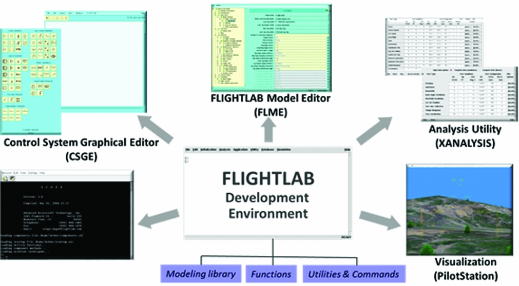
Figure A1. FLIGHTLAB development environment.

Figure A2. FLIGHTLAB Model Editor (FLME).

Figure A3. FLIGHTLAB Control System Graphical Editor (CSGE).
Xanalysis provides multiple GUIs for direct user interaction with and analysis of rotorcraft models. Xanalysis allows the user to enter commands and to execute analysis scripts and functions. In addition, a wide range of model setup and analysis functionalities such as setting test conditions and aircraft configurations, model trim and linearisation, time-marching control response, conducting simulated flight tests (e.g., hover, low speed, climb, cruise, turn, etc.), and more are provided via interactive GUIs and menus. The Flight Test GUI of Xanalysis is shown in Fig. A4. This GUI is presented in the form of a flight test card with standard rotorcraft flight tests listed in the first column. For each selected flight-test option, the user then enters the test conditions and rotorcraft configuration and defines inputs and outputs for the test. If flight-test data are available, they may be imported and overlaid with the simulation results. Xanalysis also includes a rotorcraft handling qualities analysis GUI based on the U.S. Army Rotorcraft Aeronautical Design Standard, ADS-33(22). Analysis results can be saved or plotted within Xanalysis or data can be exported for external use and visualisation.

Figure A4. Xanalysis flight test GUI.
Models developed in the FLME GUI (referred to as Development Models) are executed and analysed in the Xanalysis GUI. The model sophistication and fidelity can vary to support various aspects of aircraft modelling and analysis, including early conceptual design, detailed control system design, flight test and maintenance support, component and/or subsystem improvement studies and more. Xanalysis executes analysis scripts that use built-in functionalities or user-defined analysis to run the model through required analysis scenarios.
A.2 PilotStation
Development models can be synchronised to real-time and linked to a pilot interface with controls and displays using PilotStation. PilotStation allows an engineer to interactively fly the model in the development system to evaluate performance and handling qualities. An operator console provides control of the simulation run including setting the flight condition; modifying the vehicle configuration; trimming the rotorcraft to the initialised flight condition; initiating run, pause, and reset; and selecting data for recording during the run. Since it is executed within the development environment, PilotStation allows the user to fly the model to a specific flight condition, pause the flight simulation and interactively examine aircraft states and interface data. Model parameters and properties may also be modified while the model is paused and before continuing the run. PilotStation is therefore a powerful tool for testing a flight dynamics model and interactively modifying model parameters, such as flight control gains.
PilotStation includes a plug-in to the open-source FLIGHTGEAR image generation software. (Fig. A5). Many Open Source geo-specific terrain databases are available for use with FLIGHTGEAR and the open-Source software allows extensive customisation by the user.

Figure A5. PilotStation out-the-window display with heads-up display.
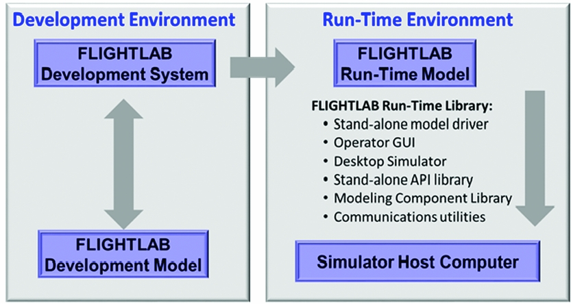
A.3 FLIGHTLAB run-time system and run-time models
In the development environment, the user has complete access to all model data and structures and can edit and analyse any aspect of the model easily and conveniently. This extensive editing and analysis capability is generally not required in a real-time application and also reduces the efficiency of real-time operations and complicates integration with a distributed computing environment. The run-time system was designed to support the integration and real-time execution of models with simulators and hardware-in-the-loop laboratories. The run-time model is a representation of the development model that is designed to support efficient integration into a distributed computational environment and efficient real-time operation through the use of the run-time system.
Run-time models are derived from development models but are designed to run independent of the development system requiring only the run-time system for execution.
The run-time system includes:
• a physics-based run-time modelling component library;
• an application programming interface (API) functions library;
• a driver that executes the run-time model and synchronises it to real-time;
• an operator GUI with remote access to the model driver commands;
• communication utilities for interfacing to the host computer through a local area network.
A schematic diagram of the development and run-time environments is shown in Fig. A6.

Figure A6. FLIGHTLAB development and run-time environments.
A.4 Simulation qualification tool (SIMQT)
The flight-test GUI in Xanalysis permits comparison of simulation and flight-test results within the development system where the model is most readily modified for calibration. Once the model is ready for use in a training simulator, it is output as a run-time model for execution in the run-time system where it is interfaced to the simulator. The FAA requires that comparisons with flight-test data be performed on the model actually used with the simulator so the tests run on the development model, although it is technically the same as the run-time model, do not satisfy this requirement. The Simulation Qualification Tool (SIMQT) is a software package to automatically perform simulated flight test scenarios on run-time models in an offline batch execution in order to satisfy this requirement. The tool includes all FAA Level D flight-test scenarios and provides FAA Level D standard-report formats.
This tool initiates the test condition from the flight-test data, drives the model with the pilot control history from the flight-test data, and provides superimposed plots of the model-test results with the reference flight-test results.
SIMQT has been implemented in multiple full-flight helicopter simulators with acceptance testing based on the FAA's Level D methodology. SIMQT can provide an onsite tool to reproduce the test results and to provide a regression test capability for these applications.
A.5 Viscous vortex particle method
VPM(Reference He and Zhao6-Reference He and Rajmohan11) is a recently developed solution dedicated to solving the vortex-wake-dominated problems for multiple rotors, wings, and ducted-fan configurations. It is a robust and computationally very efficient tool for solving complicated rotorcraft aerodynamic interaction problems. VPM is based on a first-principle formulation and efficiently solves the incompressible Navier-Stokes equation in a vorticity-velocity form with a grid-less Lagrangian representation. It accurately convects the vorticity in the flow-field without any artificial dissipation while capturing the wake distortion and physical diffusion due to viscosity. The VPM tool is best suited for modelling rotorcraft aerodynamic interaction problems, such as rotor/wing, rotor/fuselage, and rotor/superstructure. VPM is fully parallelised using Graphical Processing Units (GPUs) and the OpenMP multiprocessing software. VPM can be coupled with a lifting-line-based blade element, a lifting-surface model, or a grid-based Navier Stokes Computational Fluid Dynamics (N-S CFD) solver. In the coupled application, FLIGHTLAB or a CFD solver computes the vorticity source emanated from body surfaces and VPM transports the wake vorticity throughout the entire flow-field. The coupled VPM/CFD simulation renders a hybrid flow solver that maximises the benefits of both VPM and CFD solvers. The near-body flow-field is accurately captured using CFD while the wake-vorticity structure is well preserved using the efficient VPM simulation. Figure A7 illustrates example rotor wakes for various rotor configurations and flight conditions as predicted by VPM.

Figure A7. Example rotor wake geometries as predicted by VPM.
A.6 Virtual pilot laboratory (VPLAB)
The Virtual Pilot Laboratory (VPLAB) is a toolset to facilitate defining a control history that can fly a rotorcraft though a prescribed set of vehicle states(Reference Lee, He, Saberi and Du Val23). The tool was initially developed to support testing of avionics systems across a wide range of mission profiles. The objective was to derive a control history that could be applied to an aircraft-specific model to fly the model through a prescribed set of waypoints, orientations, and angular and translational rates and accelerations. The resulting control history is then used with the model to stimulate avionics systems through a prescribed mission scenario in a repeatable fashion. The approach is also useful in flying a comprehensive model through manoeuvring flight without requiring a pilot in the loop. This allows for manoeuvring analysis of models that cannot run in real time due to computationally intensive modelling.
The next generation of rotorcraft include designs that provide for vertical take-off and landing as a helicopter and high-speed forward flight as a fixed-wing aircraft. The transition between helicopter and fixed-wing modes provides significant control system challenges. The ability of VPLAB to generate a control history for a specific aircraft and manoeuvre combination can be useful in the design and implementation of a transition controller for a rotorcraft. The resulting control history can be used as feed forward in the controller with an added feedback loop compensating for deviations that result from environmental conditions or modelling discrepancies.
The tool includes an input processor to define the flight profile using 3D visualisation, control generation using the dynamic trim approach, and implementation of the resulting control with the standalone model in a run-time environment, as shown in Fig. A8.

Figure A8. Virtual pilot laboratory (VPLAB).
VPLAB generates the control by using inverse simulation in a dynamic trim plus a feedback control compensation process(Reference Lee, He, Saberi and Du Val23) to fly the model through a prescribed trajectory with prescribed state constraints. Discrete points are selected along the prescribed trajectory and the required acceleration at these points is determined. The model is linearised about each of these discrete points and the inverse of the linearised model is used in an iterative gradient search to compute the controls required to achieve the specified accelerations subject to any specified state constraints. If the dynamic trim fails to converge this indicates that the specified trajectory, or the specified state constraints, are beyond the performance capability of the aircraft and additional iterations on the prescribed trajectory or state constraints are required.