2.1 Navier–Stokes equations

The compressible Navier–Stokes equations were utilized to simulate the two-dimensional laminar flow past a square cylinder at low Reynolds numbers ( $Re\leqslant 200$ ). The Mach number was set to be $Ma=0.1$ . It has been confirmed that the compressible Navier–Stokes equations with Mach numbers less than 0.3 can be used as an efficient alternative to study incompressible flows as well as the flow-induced vibrations of bluff bodies (Wanderley & Levi Reference Wanderley and Levi2002). The Reynolds number, based on the oncoming flow velocity ( $U_{\infty }$ ) and the side length of the square cylinder ( $D$ ), is defined as $Re=\unicode[STIX]{x1D70C}U_{\infty }D/\unicode[STIX]{x1D707}$ , where $\unicode[STIX]{x1D70C}$ and $\unicode[STIX]{x1D707}$ are the density and the dynamic viscosity of the fluid, respectively. To cope with the deforming mesh due to the vibration of the cylinder, the arbitrary Lagrangian–Eulerian form of the Navier–Stokes equations was employed. The non-dimensional governing equations, with all physical variables normalized by $U_{\infty }$ and  $D$ , are given as follows:

(2.1) $$\begin{eqnarray}\frac{\unicode[STIX]{x2202}}{\unicode[STIX]{x2202}t}\int \int _{\unicode[STIX]{x1D6FA}}\boldsymbol{Q}\,\text{d}V+\oint _{\unicode[STIX]{x2202}\unicode[STIX]{x1D6FA}}\boldsymbol{F}(\boldsymbol{Q},\boldsymbol{V}_{grid})\boldsymbol{\cdot }\boldsymbol{n}\,\text{d}S=\oint _{\unicode[STIX]{x2202}\unicode[STIX]{x1D6FA}}\boldsymbol{G}(\boldsymbol{Q})\boldsymbol{\cdot }\boldsymbol{n}\,\text{d}S,\end{eqnarray}$$

where $\unicode[STIX]{x1D6FA}$ denotes the control surface element, $\unicode[STIX]{x2202}\unicode[STIX]{x1D6FA}$ represents the boundary of the control surface element, $t$ is the dimensionless time and $\boldsymbol{n}$ is the identity normal vector. The vector of conservative variables  $\boldsymbol{Q}$ , the modified inviscid flux vector $\boldsymbol{F}(\boldsymbol{Q},\boldsymbol{V}_{grid})$ and the viscous flux vector $\boldsymbol{G}(\boldsymbol{Q})$ are given as follows:

(2.2a,b ) $$\begin{eqnarray}\boldsymbol{Q}=\left[\begin{array}{@{}c@{}}\unicode[STIX]{x1D70C}\\ \unicode[STIX]{x1D70C}u\\ \unicode[STIX]{x1D70C}v\\ e_{0}\end{array}\right],\quad \boldsymbol{F}_{x}(\boldsymbol{Q},\boldsymbol{V}_{grid})=\left[\begin{array}{@{}c@{}}\unicode[STIX]{x1D70C}(u-u_{grid})\\ \unicode[STIX]{x1D70C}u(u-u_{grid})+P\\ \unicode[STIX]{x1D70C}(u-u_{grid})v\\ e_{0}(u-u_{grid})+Pu\end{array}\right],\end{eqnarray}$$

(2.3) $$\begin{eqnarray}\displaystyle & \displaystyle \boldsymbol{F}_{y}(\boldsymbol{Q},\boldsymbol{V}_{grid})=\left[\begin{array}{@{}c@{}}\unicode[STIX]{x1D70C}(v-v_{grid})\\ \unicode[STIX]{x1D70C}u(v-v_{grid})\\ \unicode[STIX]{x1D70C}(v-v_{grid})v+P\\ e_{0}(v-v_{grid})+Pv\end{array}\right], & \displaystyle\end{eqnarray}$$

(2.4) $$\begin{eqnarray}\displaystyle & \displaystyle \boldsymbol{G}_{x}(\boldsymbol{Q})=\unicode[STIX]{x1D707}\left[\begin{array}{@{}c@{}}0\\ 2u_{x}-{\displaystyle \frac{2}{3}}(u_{x}+v_{y})\\ v_{x}+u_{y}\\ u\left[2u_{x}-{\displaystyle \frac{2}{3}}(u_{x}+v_{y})\right]+v(v_{x}+u_{y})+{\displaystyle \frac{1}{\unicode[STIX]{x1D6FE}-1}}{\displaystyle \frac{T_{x}}{Pr}}\end{array}\right], & \displaystyle\end{eqnarray}$$

(2.5) $$\begin{eqnarray}\displaystyle & \displaystyle \boldsymbol{G}_{y}(\boldsymbol{Q})=\unicode[STIX]{x1D707}\left[\begin{array}{@{}c@{}}0\\ v_{x}+u_{y}\\ 2v_{y}-{\displaystyle \frac{2}{3}}(u_{x}+v_{y})\\ u(v_{x}+u_{y})+v\left[2v_{y}-{\displaystyle \frac{2}{3}}(u_{x}+v_{y})\right]+{\displaystyle \frac{1}{\unicode[STIX]{x1D6FE}-1}}{\displaystyle \frac{T_{y}}{Pr}}\end{array}\right], & \displaystyle\end{eqnarray}$$

where $u$ , $v$ are the $x$ -wise and $y$ -wise components of the velocity vector of the flow, $u_{grid}$ , $v_{grid}$ are the $x$ -wise and $y$ -wise components of the velocity vector of the deforming grid and $e_{0}$ , $P$ denote the total energy and pressure, respectively. The subscripts $x$ and $y$ denote the partial derivatives of the flow velocity; $T$ is the temperature, $Pr$ is the Prandtl number and $\unicode[STIX]{x1D6FE}=1.4$ is the ratio of specific heats.

The computational domain as well as the generated mesh is shown in figure 1. The overall size of the computational domain is $60D\times 40D$ , and the centre of the square cylinder is $20D$ from the upstream boundary. The unstructured hybrid mesh employed for the present computations consists of 18 741 nodes and 34 408 elements. We refer to this mesh as  $M1$ . The convergence of $M1$ has been verified by a finer mesh in § 2.3. No-slip boundary condition was applied on the velocity of the cylinder surface. The location and velocity of the cylinder were updated at each real-time step. The far field was assigned a non-reflective boundary condition using the Riemann invariants. The entire mesh was deformed at each time step and was updated using the radial base function interpolation method (Boer, Van der Schoot & Bijl Reference De Boer, Van der Schoot and Bijl2007). A compact Wendlands C2 function was chosen as the basis function. The quality of the meshes after deformation is high enough to perform accurate flow calculations.

Figure 1. Computational domain for a square cylinder: (a) hybrid mesh employed in the present study and (b) close-up view of the mesh near the surface of the cylinder.

2.2 Structure motion equation

In this study, we focus on the dynamic response characteristics of an elastically mounted square cylinder subjected to a uniform flow, as sketched in figure 2. The square cylinder is free to vibrate in the transverse direction only. The rigid motion of the body along the Cartesian axes is given by:

(2.6) $$\begin{eqnarray}\ddot{Y} +4\unicode[STIX]{x03C0}F_{s}\unicode[STIX]{x1D701}{\dot{Y}}+(2\unicode[STIX]{x03C0}F_{s})^{2}Y=\frac{C_{L}}{2m^{\ast }},\end{eqnarray}$$

where $F_{s}=f_{s}D/U_{\infty }$ is the reduced natural frequency in a vacuum related to the natural frequency of a mass–spring system ( $f_{s}$ ); $\unicode[STIX]{x1D701}$ is the structural damping ratio and is set to be zero to encourage large-amplitude oscillations; $m^{\ast }$ is the non-dimensional mass of the body defined as $m^{\ast }=m/\unicode[STIX]{x1D70C}D^{2}$ with $m$ the actual mass of the oscillator per unit length; $C_{L}$ is the instantaneous lift coefficient acting on the body; $\ddot{Y}$ , ${\dot{Y}}$ and $Y$ denote the acceleration, velocity and displacement of the cylinder in the transverse direction normalized by $D$ and $U_{\infty }$ . In particular, the reduced velocity is defined as $U^{\ast }=1/F_{s}=U_{\infty }/f_{s}D$ .

Figure 2. Schematic diagram of an elastically mounted square cylinder subjected to a uniform flow; $m$ , $c$ and $k$ are the mass, damping and stiffness of the system.

2.3 Numerical scheme and verification

The cell-centred finite volume method was employed to solve the Navier–Stokes equations. Spatial discretization of the inviscid flux terms was accomplished using the second-order AUSM+-up scheme (Liou Reference Liou2006), while the viscous flux terms were discretized by the standard central scheme. A second-order accurate full implicit scheme was used to integrate the equations in time domain, and an implicit symmetric Gauss–Seidel iterative time-marching scheme was applied in the pseudo time step.

A fourth-order hybrid linear multi-step scheme was adopted to solve the nonlinear FSI problems (Zhang, Jiang & Ye Reference Zhang, Jiang and Ye2007). The flow and structural equations were solved separately using a partitioned approach. At each real-time step, the fluid force acting on the square cylinder was obtained from the solution of Navier–Stokes equations; and then the displacement of the inner boundary was updated by solving the structural motion equation, which was necessary for the solution of the flow equations at the next time step. A more detailed process and extensive validations of the numerical method have been documented in our previous works (Zhang et al. Reference Zhang, Li, Ye and Jiang2015a ; Li, Zhang & Gao Reference Li, Zhang and Gao2018). For completeness, further validations of the numerical method for the flow and VIV of a square cylinder at low $Re$ were performed. Mesh dependency and time step convergence study was also carried out.

Firstly, we computed the flow past a stationary square cylinder at $Re=100$ . To study the convergence of the time step, four computations were conducted at $\unicode[STIX]{x0394}t=0.20$ , 0.10, 0.05 and 0.02 for  $M1$ . In addition, a finer mesh $M2$ with 24 764 nodes and 44 648 elements was generated for the mesh dependency study; $M2$ has the same domain size as $M1$ but has higher spatial resolution especially close to the surface of the square cylinder. Table 1 shows the comparison of the mean drag coefficient ( $\overline{C_{D}}$ ), root-mean-square (r.m.s.) drag coefficient ( $C_{D}^{rms}$ ), amplitude of lift coefficient ( $C_{L}^{max}$ ), r.m.s. lift coefficient ( $C_{L}^{rms}$ ) and Strouhal number of the vortex shedding ( $St$ ) with the published results in the literature. As can be seen, with the decrease of the time step, the results for $M1$ gradually converge and remain almost unchanged when $\unicode[STIX]{x0394}t\leqslant 0.05$ . Thus, the time step was set to be $\unicode[STIX]{x0394}t=0.05$ for most of the present computations. On the other hand, the results from $M1$ and $M2$ at $\unicode[STIX]{x0394}t=0.05$ are in good agreement and the differences of the values between the two meshes are generally less than 1 %. This indicates that $M1$ is adequate for the present study. Besides, our results compare reasonably well with those of other researchers, verifying that the numerical method we adopted is reliable.

Table 1. Mesh dependency and time step convergence study: comparison of the present calculation results with the published numerical data in the literature for the flow past a stationary square cylinder at $Re=100$ .

To further verify our numerical solver, VIV of a square cylinder with two degrees of freedom was simulated. The parameter settings were consistent with one of the numerical cases in Zhao et al. (Reference Zhao, Cheng and Zhou2013), i.e. $Re=100$ , $m^{\ast }=3$ and $\unicode[STIX]{x1D701}=0$ . The square cylinder is free to vibrate in both the transverse and in-line directions. The reduced velocity $U^{\ast }$ is varied by changing the reduced natural frequency of the structure $F_{s}$ . Since the vibration amplitude in the transverse direction is much larger than that in the in-line direction, we only present the results for transverse vibrations. Figure 3 shows the transverse vibration amplitude of the cylinder varying with  $U^{\ast }$ . The vibration amplitude in the transverse direction is defined as $A_{y}=(Y^{max}-Y^{min})/2$ with $Y^{max}$ and $Y^{min}$ being the maximum and minimum transverse displacements of the cylinder, respectively. As can be seen, remarkable VIV begins to occur at $U^{\ast }=4$ , and the response amplitude increases rapidly in the range $4<U^{\ast }<5$ . The maximum vibration amplitude is achieved at $U^{\ast }=5$ , approximately, with a value of $A_{y}=0.315$ . When $U^{\ast }>5$ , the transverse vibration amplitude decreases gradually with the increase of  $U^{\ast }$ . It is worth noting that the critical reduced velocity for vortex-shedding resonance $U_{r}^{\ast }=1/St$ falls in the descending branch of the VIV response. Moreover, as will be shown in figure 8(b), when the mass ratio is further reduced, the response curve of VIV expands on the left-hand side of $U_{r}^{\ast }$ . This is opposite to the cases of high Reynolds numbers and high mass ratios, for which $U_{r}^{\ast }$ falls at the beginning of the VIV response pattern and the excitation range expands on the right-hand side (Bearman & Obasaju Reference Bearman and Obasaju1982; Nakamura & Matsukawa Reference Nakamura and Matsukawa1987).

Figure 3. Transverse vibration amplitude for VIV of a two-degree-of-freedom elastically mounted square cylinder at $Re=100$ , $m^{\ast }=3$ and $\unicode[STIX]{x1D701}=0$ . The numerical results of Zhao et al. (Reference Zhao, Cheng and Zhou2013) are also plotted for comparison; $U_{r}^{\ast }=1/St$ denotes the critical reduced velocity for vortex-shedding resonance.

The present numerical results agree excellently well with those of Zhao et al. (Reference Zhao, Cheng and Zhou2013). This indicates that our numerical method is effective and applicable to study the FIV problems of a square cylinder at low  $Re$ .

3.1 Reduced-order modelling of the unsteady wake flow

The model reduction for unsteady flow has been an active area of research in recent years (Lucia, Beran & Silva Reference Lucia, Beran and Silva2004; Ghoreyshi, Jirasek & Cummings Reference Ghoreyshi, Jirasek and Cummings2014; Rowley & Dawson Reference Rowley and Dawson2017). Compared to high-fidelity numerical simulations, reduced-order models (ROMs) can retain the dominant flow dynamics of the original system with significant lower orders, which results in a great improvement of computational efficiency. In this section, we focus on developing ROMs for the unsteady flow past a transversely vibrating square cylinder. The system identification method based on the ARX model was adopted for model reduction. This method has been discussed in detail in our previous works (Zhang et al. Reference Zhang, Li, Ye and Jiang2015a ; Gao et al. Reference Gao, Zhang, Li, Liu, Quan, Ye and Jiang2017; Kou & Zhang Reference Kou and Zhang2019). For completeness, we give a brief introduction of the ROM method here. The linear time-invariant input–output model is given as:

(3.1) $$\begin{eqnarray}\boldsymbol{y}_{F}(k)=\mathop{\sum }_{i=1}^{na}\unicode[STIX]{x1D63C}_{i}\boldsymbol{y}_{F}(k-i)+\mathop{\sum }_{i=0}^{nb-1}\unicode[STIX]{x1D63D}_{i}\boldsymbol{u}(k-i),\end{eqnarray}$$

where $\boldsymbol{y}_{F}$ is the output vector and $\boldsymbol{u}$ is the input vector of the system. For the current single-input–single-output model, $\boldsymbol{u}=[Y]$ (transverse displacement) and $\boldsymbol{y}_{F}=[C_{L}]$ (instantaneous lift coefficient); $\unicode[STIX]{x1D63C}_{i}$ and $\unicode[STIX]{x1D63D}_{i}$ are the constant coefficients to be estimated. The least squares method is employed for the estimation procedure; $na$ and $nb$ are the delay orders determined by the user. By varying $na$ and  $nb$ , we can find the model that minimizes the error between the training data and ROM predictions.

Figure 4. Steady-state base flow of a stationary square cylinder at $Re=150$ : (a) streamwise and (b) cross-flow velocity fields.

Figure 5. (a)Time history and (b) fast Fourier transformation of the training signal.

The discrete-time fluid model (3.1) can be further converted into the continuous-time state-space form as:

(3.2) $$\begin{eqnarray}\left.\begin{array}{@{}l@{}}\dot{\boldsymbol{x}}_{F}(t)=\unicode[STIX]{x1D63C}_{F}\boldsymbol{x}_{F}(t)+\unicode[STIX]{x1D63D}_{F}u(t),\\ y_{F}(t)=\unicode[STIX]{x1D63E}_{F}\boldsymbol{x}_{F}(t)+\unicode[STIX]{x1D63F}_{F}u(t),\end{array}\right\}\end{eqnarray}$$

where $\boldsymbol{x}_{F}$ is the state vector with the order of $(na+nb)$ ; $(\unicode[STIX]{x1D63C}_{F},\unicode[STIX]{x1D63D}_{F},\unicode[STIX]{x1D63E}_{F},\unicode[STIX]{x1D63F}_{F})$ are the system matrices. Once the ROM is established, the stability characteristics of the flow can be quickly obtained by computing the eigenvalues of matrix $\unicode[STIX]{x1D63C}_{F}$ in the state-space equation (3.2). It is remarkable that, for the stable flow at subcritical $Re$ , the ROM can be directly identified based on the steady flow. However, for the unstable flow at supercritical $Re$ , the ROM should be trained based on the unstable steady-state base flow.

Here, we take the unsteady flow modelling of $Re=150$ as an example to verify the correctness of the ROM method. The steady-state base flow was computed using a time-filtering method based on the unsteady flow solver (Zhang, Liu & Li Reference Zhang, Liu and Li2015b ), as shown in figure 4. A smoothed chirp signal with an increasing frequency is adopted as the training signal. The time history as well as the fast Fourier transformation (FFT) of the signal is shown in figure 5. As can be seen, the signal has a wide reduced frequency band ranging from 0 to 0.4 approximately, which covers the vortex-shedding frequency of a square cylinder in the laminar flow regime. When the data training is completed, we vary the delay orders to construct an accurate enough model. The identification error used for model-order selection is defined as:

(3.3) $$\begin{eqnarray}e=\frac{\displaystyle \mathop{\sum }_{i=1}^{N}|y_{F}(i)-y_{F}^{iden}(i)|}{\displaystyle \mathop{\sum }_{i=1}^{N}|y_{F}(i)|},\end{eqnarray}$$

where $y_{F}^{iden}$ denotes the vector of the identified lift coefficient and $N$ is the size of the training data. The identified results with various delay orders are compared with those of direct numerical simulation in figure 6. For clarity, only the results for $na=nb$ are presented. As can be seen, the identification error gradually decreases with increasing delay orders. The best identification is achieved at $na=nb=80$ with an identification error less than 1 %. Hence, for the case of $Re=150$ , we set the delay orders equal to $na=nb=80$ .

Figure 6. Identified results under the training signal compared with that of direct numerical simulation at $Re=150$ .

For further verification, the ARX-based ROM was applied to predict the instability onset of the square cylinder wake flow due to a Hopf bifurcation. The eigenvalues of the first two least-stable modes at various Reynolds numbers are plotted in figure 7. As can be seen, the base flow starts to become unstable at $Re_{cr}\approx 45.2$ when the eigenvalue of the leading fluid mode crosses the imaginary axis and moves into the right half of the complex plane, which is consistent with the numerical predictions of Yoon, Yang & Choi (Reference Yoon, Yang and Choi2010), Park & Yang (Reference Park and Yang2016) and Yao & Jaiman (Reference Yao and Jaiman2017). In addition, the eigenvalue of the second fluid mode gradually approaches the imaginary axis as the $Re$ increases. This indicates that the second mode tends to be a weak-stable mode (light-damped mode) at large $Re$ , and therefore cannot be neglected anymore in fluid-elastic stability analysis. We will show in § 5 that the second fluid mode plays an important role in the fluid–structure coupling mechanism that inherently leads to the galloping-type oscillation of the structure.

Figure 7. Eigenvalue analysis via the ARX-based ROM for the flow past a stationary square cylinder: (a) least-stable fluid mode and (b) second least-stable fluid mode. The flow becomes unstable at the critical $Re_{cr}=45.2$ when the eigenvalue of the least-stable fluid mode crosses the imaginary axis and moves into the right half of the complex plane.

3.2 ROM-based FSI model

By defining a structure state vector $\boldsymbol{x}_{s}=[Y,{\dot{Y}}]^{T}$ for the present one-degree-of-freedom transversely vibrating square cylinder, the structure motion equation (2.6) can be written in the state-space form as:

(3.4) $$\begin{eqnarray}\left.\begin{array}{@{}l@{}}\dot{\boldsymbol{x}}_{S}(t)=\unicode[STIX]{x1D63C}_{S}\boldsymbol{x}_{S}(t)+q\unicode[STIX]{x1D63D}_{S}y_{F}(t),\\ Y(t)=\unicode[STIX]{x1D63E}_{S}\boldsymbol{x}_{S}(t)+q\unicode[STIX]{x1D63F}_{S}y_{F}(t),\end{array}\right\}\end{eqnarray}$$

where $\unicode[STIX]{x1D63C}_{S}=\left[\!\begin{smallmatrix}0 & 1\\ -(2\unicode[STIX]{x03C0}F_{s})^{2} & -4\unicode[STIX]{x03C0}F_{s}\unicode[STIX]{x1D701}\end{smallmatrix}\!\right]$ , $\unicode[STIX]{x1D63D}_{S}=\left[\!\begin{smallmatrix}0\\ 1\end{smallmatrix}\!\right]$ , $\unicode[STIX]{x1D63E}_{S}=\left[\!\begin{smallmatrix}1 & 0\end{smallmatrix}\!\right]$ , $\unicode[STIX]{x1D63F}_{S}=\left[\!\begin{smallmatrix}0\end{smallmatrix}\!\right]$ and $q=1/(2m^{\ast })$ . By coupling the structural state equation (3.4) with the aerodynamic state equation (3.2), we obtain the state and output equations for the linear coupled system as follows:

(3.5) $$\begin{eqnarray}\left.\begin{array}{@{}c@{}}\dot{\boldsymbol{x}}_{FS}(t)=\left[\begin{array}{@{}cc@{}}\unicode[STIX]{x1D63C}_{S}+q\unicode[STIX]{x1D63D}_{S}\unicode[STIX]{x1D63F}_{F}\unicode[STIX]{x1D63E}_{S} & q\unicode[STIX]{x1D63D}_{S}\unicode[STIX]{x1D63E}_{F}\\ \unicode[STIX]{x1D63D}_{F}\unicode[STIX]{x1D63E}_{S} & \unicode[STIX]{x1D63C}_{F}\end{array}\right]\boldsymbol{\cdot }\boldsymbol{x}_{FS}=\unicode[STIX]{x1D63C}_{FS}\unicode[STIX]{x1D66D}_{FS}(t)\\ Y(t)=[\unicode[STIX]{x1D63E}_{S},\unicode[STIX]{x1D7EC}]\boldsymbol{\cdot }\boldsymbol{x}_{FS}(t),\end{array}\right\}\end{eqnarray}$$

where $\boldsymbol{x}_{FS}=[\boldsymbol{x}_{S},\boldsymbol{x}_{F}]^{T}$ . The ROM-based linear dynamic model for FIV of a square cylinder is now constructed. The fluid-elastic stability problem is then converted into solving and analysing the eigenvalues of $\unicode[STIX]{x1D63C}_{FS}$ , expressed as $\unicode[STIX]{x1D706}=\unicode[STIX]{x1D706}_{r}+\text{i}\unicode[STIX]{x1D706}_{i}$ . The real part $\unicode[STIX]{x1D706}_{r}$ represents the growth rate of the eigenmodes, while the imaginary part $\unicode[STIX]{x1D706}_{i}$ denotes the angular frequency, which is equal to $2\unicode[STIX]{x03C0}$ times the eigenfrequency of the eigenmodes. Tracking the eigenvalues varying with structural parameters ( $F_{s}$ , $\unicode[STIX]{x1D701}$ and  $m^{\ast }$ ), we can obtain the stability characteristics of the coupled system. Specifically, in the present study, we investigate the trajectories of eigenvalues by varying the reduced natural frequency of structure $F_{s}$ ( $1/U^{\ast }$ ) while maintaining the $Re$ , $m^{\ast }$ and $\unicode[STIX]{x1D701}$ fixed at given values.

4.1 Response amplitude

The transverse vibration amplitudes of the square cylinder as a function of $U^{\ast }$ at various $(Re,m^{\ast })$ combinations are shown in figure 8. Figure 8(a) shows the results for $m^{\ast }=10$ at four representative Reynolds numbers, $Re=140$ , 150, 160 and 180. Figure 8(b) shows the results for $Re=150$ at four representative mass ratios, $m^{\ast }=2$ , 5, 10 and 20. Overall, there exist two typical FIV responses: VIV and galloping. When the structure natural frequency approaches the vortex-shedding frequency of a stationary cylinder in the range $4<U^{\ast }<8$ , vortex-excited resonance leads to a relatively large-amplitude vibration of the structure. Compared to its circular cylinder counterpart, the vibration amplitude and lock-in regime for VIV of a square cylinder are much smaller and narrower, which is in agreement with the numerical results of Sen & Mittal (Reference Sen and Mittal2011). This is mainly because VIV of a square cylinder is dominated by resonance without any flutter regime (Yao & Jaiman Reference Yao and Jaiman2017). As demonstrated in Zhang et al. (Reference Zhang, Li, Ye and Jiang2015a ), flutter is the root cause of frequency lock-in, which can lead to larger vibration amplitude of the structure than that induced by resonance. Galloping mainly occurs at relatively large reduced velocities, generally $U^{\ast }>10$ . When the reduced velocity is greater than a critical threshold $U_{g}^{\ast }$ , the transverse vibration amplitude increases progressively with the increase of  $U^{\ast }$ . Unlike VIV, which only shows large-amplitude oscillations in the lock-in region, galloping is a kind of unbounded vibration. There exists no upper instability boundary with regard to $U^{\ast }$ beyond which galloping will cease.

Figure 8. Transverse vibration amplitude of the square cylinder as a function of $U^{\ast }$ for various $(Re,m^{\ast })$ combinations: (a) results for $m^{\ast }=10$ at different $Re$ and (b) results for $Re=150$ at different  $m^{\ast }$ . Note that the results for $(Re,m^{\ast })=(150,10)$ are shown in both plots.

For the case of $m^{\ast }=10$ , the response amplitude of VIV decreases slightly as the $Re$ increases. Moreover, the reduced velocity corresponding to the peak value of vibration amplitude varies little with $Re$ and locates at $U^{\ast }=5.75$ , approximately. On the other side, the galloping onset $U_{g}^{\ast }$ decreases gradually and the galloping vibration amplitude increases monotonically with increasing $Re$ . It is noteworthy that there is a kink in the amplitude response of $Re=180$ near $U^{\ast }=16$ (figure 8 a). This phenomenon has been previously investigated by Zhao et al. (Reference Zhao, Leontini, Jacono and Sheridan2014) and Jaiman, Guan & Miyanawala (Reference Jaiman, Guan and Miyanawala2016), and is attributed to the 1 : 3 synchronization between the vortex-shedding frequency and the body oscillation frequency. With the increase of $Re$ , the onset of galloping gradually extends to lower reduced velocities where the unsteady effect is very strong. For the present study in the laminar flow regime, VIV and galloping are always separated with a desynchronization region between them. No combined VIV–galloping phenomenon is observed. It is remarkable that the vibration amplitude of galloping drops suddenly when the Reynolds number is reduced from 150 to 140. This indicates the existence of a critical $Re$ below which galloping will not occur. To accurately determine the critical $Re$ , further computations were conducted for various $Re$ at a sufficiently large reduced velocity $U^{\ast }=40$ . Figure 9 shows the vibration amplitude of the cylinder as a function of $Re$ . As can be seen, the critical Reynolds number $Re_{cg}$ for galloping is approximately 139, which is close to the value of 140 predicted by Joly et al. (Reference Joly, Etienne and Pelletier2012).

Figure 9. Variation of the transverse vibration amplitude with $Re$ for $m^{\ast }=10$ at a sufficiently large $U^{\ast }=40$ .

For the case of $Re=150$ , with the decrease of $m^{\ast }$ , the resonance peak of VIV gradually increases while the corresponding reduced velocity $U^{\ast }$ where the peak is acquired slightly decreases. This indicates that VIV is intensified when the mass ratio is decreased. In contrast, the onset of galloping increases and the galloping vibration amplitude decreases rapidly with decrease in  $m^{\ast }$ . This is a bit counter-intuitive since the intensity of galloping oscillation is reduced as the mass ratio decreases. More specifically, the galloping-type oscillation completely vanishes for $m^{\ast }=2$ . This indicates that there exists a critical mass ratio below which galloping completely disappears and the response will be dominated by VIV only. This phenomenon was first reported by Joly et al. (Reference Joly, Etienne and Pelletier2012) and then confirmed by Sen & Mittal (Reference Sen and Mittal2015) through numerical simulations. However, as far as we know, the primary cause that leads to this strange phenomenon has not been thoroughly investigated and discussed until now. In this study, we try to give an explanation for this peculiar phenomenon from the point view of mode competition between the fluid and the structure, as will be shown in § 5.

4.2 Frequency characteristics and lift force

Here, we take the case of $(Re,m^{\ast })=(150,10)$ as an example, to further study other aspects of galloping response. Figure 10 presents the vibration amplitude  $A_{y}$ , frequency ratios of vibration and vortex shedding $F^{\ast }=F/F_{s}$ , amplitude of lift coefficient $C_{L}^{max}$ and phase angle $\unicode[STIX]{x1D719}$ between the lift coefficient $C_{L}$ and transverse displacement $Y$ , as a function of  $U^{\ast }$ . Figure 11 shows the time histories of the lift coefficient and transverse displacement as well as their power spectral densities (PSDs) at three typical  $U^{\ast }$ . As can be seen, the response can be divided into three branches by two critical reduced velocities ( $U^{\ast }=5.75$ and $U^{\ast }=17$ ): the initial branch ( $U^{\ast }\leqslant 5.75$ ), the lower branch ( $5.75<U^{\ast }<17$ ) and the galloping branch ( $U^{\ast }\geqslant 17$ ). The first two branches belong to VIV. In the initial branch, the vibration amplitude increases rapidly with increasing  $U^{\ast }$ , and the maximum vibration amplitude is acquired at $U^{\ast }=5.75$ with a value of 0.138. In the lower branch, the vibration amplitude decreases gradually with increasing  $U^{\ast }$ . When the galloping is triggered at $U_{g}^{\ast }=17$ , the vibration amplitude increases monotonously again with increasing  $U^{\ast }$ .

Figure 10. FIV response of a transversely vibrating square cylinder as a function of $U^{\ast }$ for $(Re,m^{\ast })=(150,10)$ : (a) the vibration amplitude of cylinder  $A_{y}$ , (b) the amplitude of lift coefficient $C_{L}^{max}$ , (c) the dominant frequency ratios of cylinder vibration $F_{y}^{\ast }$ and lift coefficient $F_{C_{L}}^{\ast }$ , and (d) the phase angle $\unicode[STIX]{x1D719}$ between $C_{L}$ and $Y$ at the vibration frequency. The frequency ratio is defined as $F^{\ast }=F/F_{s}$ with $F_{s}$ being the reduced natural frequency of the structure.

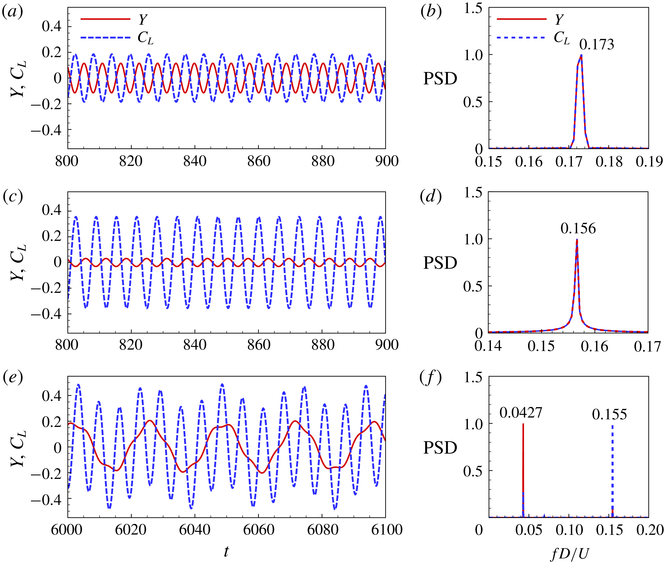
Figure 11. Time histories of transverse displacement and lift coefficient, and their power spectral densities for $(Re,m^{\ast })=(150,10)$ at three representative reduced velocities: (a,b)  $U^{\ast }=6$ , (c,d)  $U^{\ast }=10$ and (e,f)  $U^{\ast }=20$ . The power spectra are normalized by peak values.

As can be seen from figures 10(c) and 11(a–d), in the VIV region, the dominant frequencies of vortex shedding and cylinder vibration are always identical. In a very narrow region $5.75\leqslant U^{\ast }\leqslant 6.5$ , they are both synchronized with the natural frequency of the structure, i.e. the classical lock-in phenomenon occurs. Outside the lock-in region, the vibration frequency and the vortex-shedding frequency for VIV are nearly equal to the vortex-shedding frequency of a stationary square cylinder. In the galloping branch, the dominant frequencies of vortex shedding and cylinder vibration are not synchronized but become well separated. A typical response for galloping is presented in figure 11(e). From the PSD results in figure 11(f), we can see that both the fluctuating lift and vibration displacement contain two distinct frequency components, which correspond to the natural frequency of the structure and the vortex-shedding frequency of a stationary square cylinder, respectively. The dominant vibration frequency is close to, but slightly lower than the structural natural frequency in vacuum ( $F_{y}/F_{s}\approx 0.83$ ), while the dominant vortex-shedding frequency is consistent with the vortex-shedding frequency of a stationary square cylinder. The difference between the vibration frequency and the natural frequency of the structure is attributed to the added mass effect. According to Khalak & Williamson (Reference Khalak and Williamson1999), the effective added mass coefficient for a freely vibrating cylinder can be represented by

(4.1) $$\begin{eqnarray}C_{EA}=\frac{1}{2\unicode[STIX]{x03C0}^{3}}\frac{C_{L}^{\prime }\cos \unicode[STIX]{x1D719}}{A_{y}^{\prime }}\left[\frac{U_{\infty }}{f_{s}D}\right]^{2},\end{eqnarray}$$

where $C_{L}^{\prime }$ is the lift coefficient amplitude, $A_{y}^{\prime }$ is the oscillation amplitude and $\unicode[STIX]{x1D719}$ is the phase angle between the lift coefficient and transverse displacement at the dominant oscillation frequency. These values can be obtained by standard Fourier analysis using the numerical simulation data. When $C_{EA}$ is evaluated, the structural natural frequency with consideration of added mass effect can be given as

(4.2) $$\begin{eqnarray}F_{sa}=\sqrt{\frac{m^{\ast }}{m^{\ast }+C_{EA}}}\cdot F_{s}.\end{eqnarray}$$

Figure 12 shows the variation of $C_{EA}$ and the modified frequency ratio $F_{y}/F_{sa}$ with $U^{\ast }$ in the galloping regime. As can be seen, the effective added mass coefficient measured from numerical results remains around 3.3, which is close to the value of 3.5 reported in Joly et al. (Reference Joly, Etienne and Pelletier2012) for a freely oscillating square cylinder at $Re=200$ . From figure 12(b), we can see that the dominant vibration frequency of the cylinder matches exactly the natural frequency of the structure when the effective added mass is considered. The above analysis indicates that, for galloping responses, the structure vibration and the vortex shedding are basically decoupled, and they only interfere with each other by means of forced excitation.

Figure 12. (a) Effective added mass coefficient $C_{EA}$ and (b) modified frequency ratio $F_{y}/F_{sa}$ as a function of $U^{\ast }$ for $(Re,m^{\ast })=(150,10)$ in the galloping regime.

The amplitude of the lift coefficient is closely related to the phase angle between $C_{L}$ and  $Y$ , as demonstrated in figure 10(b,d). The phase angle jumps suddenly from $0^{\circ }$ to $180^{\circ }$ in the lock-in region around $U^{\ast }=5.75$ , where $C_{L}^{max}$ achieves the minimum value. This phenomenon has also been observed in the experimental study of Khalak & Williamson (Reference Khalak and Williamson1999). They indicated that the phase change through resonance is matched by a switch in the timing of vortex shedding. After the phase transition point, $C_{L}^{max}$ increases gradually with increasing  $U^{\ast }$ . However, the phase angle undergoes an abrupt change again from $180^{\circ }$ to $0^{\circ }$ around $U^{\ast }=17$ due to the occurrence of galloping instability. As evident from figure 11(e), during galloping, the low-frequency oscillation of $C_{L}$ is in phase with the vibration of the cylinder. Besides, the amplitude of the lift coefficient $C_{L}^{max}$ experiences a relatively small increase near the galloping onset.

4.3 Wake pattern

Figures 13 and 14 show the vorticity fields at typical reduced velocities for VIV ( $U^{\ast }=6$ and $U^{\ast }=10$ ) and galloping ( $U^{\ast }=20$ ), respectively. The classical terminology of Williamson & Roshko (Reference Williamson and Roshko1988) is employed to identify the wake patterns. As can be seen, for VIV responses, all the wakes present as the 2S mode (two single vortices shed during a vibration cycle). For the galloping response, the wake characteristics have no essential difference with those of VIV. However, because the vibration frequency of the cylinder is much lower than the vortex-shedding frequency, there are multiple vortex-shedding cycles during a single vibration period. Within one cycle of oscillation, the vortex-shedding structures in different vortex-shedding periods are very similar to each other. We refer to this kind of wake pattern as N(2S) mode with $\text{N}=F_{vs}/F_{y}$ , where $F_{vs}$ is the vortex-shedding frequency and $F_{y}$ is the vibration frequency of the square cylinder. As shown in figure 14(a), for the case of $U^{\ast }=20$ , N equals to 4, approximately. Thus, the wake for $U^{\ast }=20$ is referred to as the 4(2S) mode.

5.1 Clarification of modes

In the earlier studies on LSA for VIV of bluff bodies (Cossu & Morino Reference Cossu and Morino2000; Meliga & Chomaz Reference Meliga and Chomaz2011), the eigenmodes of coupled systems were classified based on their characteristics in the limit of very large mass ratios, wherein the fluid–structure coupling effect is very weak. The strength of fluid–structure coupling increases with the decrease of mass ratio (Yao & Jaiman Reference Yao and Jaiman2017). It is demonstrated that for large $m^{\ast }$ , the two leading modes are absolutely distinct for all  $U^{\ast }$ , i.e. the two modes are decoupled. Cossu & Morino (Reference Cossu and Morino2000) referred to these two modes as the ‘nearly’ structure mode and the von Kármán mode, and subsequently Meliga & Chomaz (Reference Meliga and Chomaz2011) renamed them the structure mode (SM) and the wake mode (WM), respectively. The frequency of the SM is close to the natural frequency of the structure, while the eigenvalue of the WM tends to the leading eigenvalue of the flow past a stationary cylinder. However, for sufficiently low  $m^{\ast }$ , the two leading modes may transform into mixed or coupled modes (Zhang et al. Reference Zhang, Li, Ye and Jiang2015a ; Navrose & Mittal Reference Mittal2016; Yao & Jaiman Reference Yao and Jaiman2017). They exchange roles in the synchronization region when their eigenfrequencies approach each other. Navrose & Mittal (Reference Mittal2016) defined such coupled modes as fluid-elastic mode I (FEMI) and fluid-elastic mode II (FEMII), respectively. FEMI resembles the WM at low $U^{\ast }$ while resembles the SM at large  $U^{\ast }$ . FEMII does the opposite.

Figure 15. Root loci of the coupled system as a function of $U^{\ast }$ for $Re=150$ at two representative mass ratios: (a)  $m^{\ast }=10$ and (b)  $m^{\ast }=50$ .

To classify the eigenmodes of the present FIV system, a systematic analysis is conducted by tracking the eigenvalues of the linear coupled model for a range of $U^{\ast }$ , while maintaining $Re$ and $m^{\ast }$ fixed. Figure 15 presents the eigenvalues of the three leading modes of the coupled system for $Re=150$ at two typical mass ratios, $m^{\ast }=10$ and $m^{\ast }=50$ . The corresponding growth rates and frequencies of the eigenmodes as a function of $U^{\ast }$ are plotted in figure 16. It can be seen that, for a relatively large mass ratio, $m^{\ast }=50$ , the three modes are well decoupled. According to their frequency characteristics, we define them as the wake mode I (WM-I), wake mode II (WM-II) and structure mode (SM), respectively. WM-I and WM-II tend to the leading eigenvalues of the flow past a stationary square cylinder, respectively. The modes responsible for the global instability of the fluid-only system are denoted as the stationary modes, marked by red diamonds in figure 15. On the other hand, the eigenfrequency ratio of the SM is almost constant and equals unity throughout the $U^{\ast }$ investigated (figure 16 d). This implies that the frequency of the SM follows the natural frequency of the structure. For a relatively low $m^{\ast }=10$ , the leading mode remains unchanged, still behaves as WM-I. However, the second and the third modes are coupled and exchange roles in the process of increasing  $U^{\ast }$ . This is clearly demonstrated in figure 16(c) where the frequencies of the eigenmodes are plotted against  $U^{\ast }$ , frequency transition of the two modes occurs when their eigenfrequencies get close to each other in the range $7\leqslant U^{\ast }\leqslant 9$ . Thus, they cannot be simply classified as SM or WM-II. In this study, we define them as coupled mode I (CM-I) and coupled mode II (CM-II), respectively. CM-I acts as the WM-II at low $U^{\ast }$ but acts as the SM at large  $U^{\ast }$ . On the contrary, CM-II acts as the SM at low $U^{\ast }$ while acts as the WM-II at large  $U^{\ast }$ .

Figure 16. Growth rates $\unicode[STIX]{x1D706}_{r}$ and frequency ratios $F_{LSA}^{\ast }$ of the eigenmodes as a function of $U^{\ast }$ for (a,c)  $m^{\ast }=10$ and (b,d)  $m^{\ast }=50$ . The eigenfrequency ratio is defined as $F_{LSA}^{\ast }=\unicode[STIX]{x1D706}_{i}/(2\unicode[STIX]{x03C0}F_{s})$ .

It is worth noting that, for $m^{\ast }=10$ , the eigenfrequency ratio of CM-I for $U^{\ast }>U_{c}^{\ast }$ (in this region, CM-I behaves as SM) deviates considerably from unity due to the added mass effect (figure 16 c), as discussed in § 4.2. Besides, the results from the two typical mass ratios indicate that there exists a critical mass ratio, below which the two distinct modes develop into mixed modes. For $Re=150$ , the critical mass ratio is $m_{cr}^{\ast }=32$ , approximately.

5.2 Primary cause of galloping

The mechanisms underlying galloping are investigated in this section from the perspective of linear dynamics. As can be seen from figure 15, the leading fluid mode WM-I is located in the right half of the complex plane and is therefore always unstable. It is in the shape of a ring, accumulating around the leading eigenvalue of the flow past a stationary square cylinder, and is almost unaffected by $U^{\ast }$ and  $m^{\ast }$ . This implies that its coupling with SM is very weak, which explains why the oscillation of the structure and the vortex shedding in the wake are essentially decoupled during the galloping. In contrast, the SM has a relatively strong coupling with the second fluid mode WM-II. For $m^{\ast }=50$ , the eigenvalue of SM gradually moves downwards and approaches that of WM-II as the $U^{\ast }$ increases. In this process, the coupling between SM and WM-II is enhanced. The two modes first attract and then repel each other in the interference region. Importantly, due to the repelling effect, the SM becomes unstable beyond a critical reduced velocity $U_{c}^{\ast }=9.54$ . For $m^{\ast }=10$ , the coupling between SM and WM-II becomes stronger, which ultimately leads to the mode transition phenomenon. The two distinct modes change into coupled modes as CM-I and CM-II, respectively. CM-II is always stable while CM-I becomes unstable beyond $U_{c}^{\ast }=7.85$ . Since CM-I practically behaves as SM in the whole unstable region $U^{\ast }>U_{c}^{\ast }$ , and to give a more comprehensible explanation, we use SM instead of CM-I for further discussion of the galloping mechanism in the following parts of this paper. We suppose that the instability of SM may be closely related to the occurrence of galloping-type oscillation.

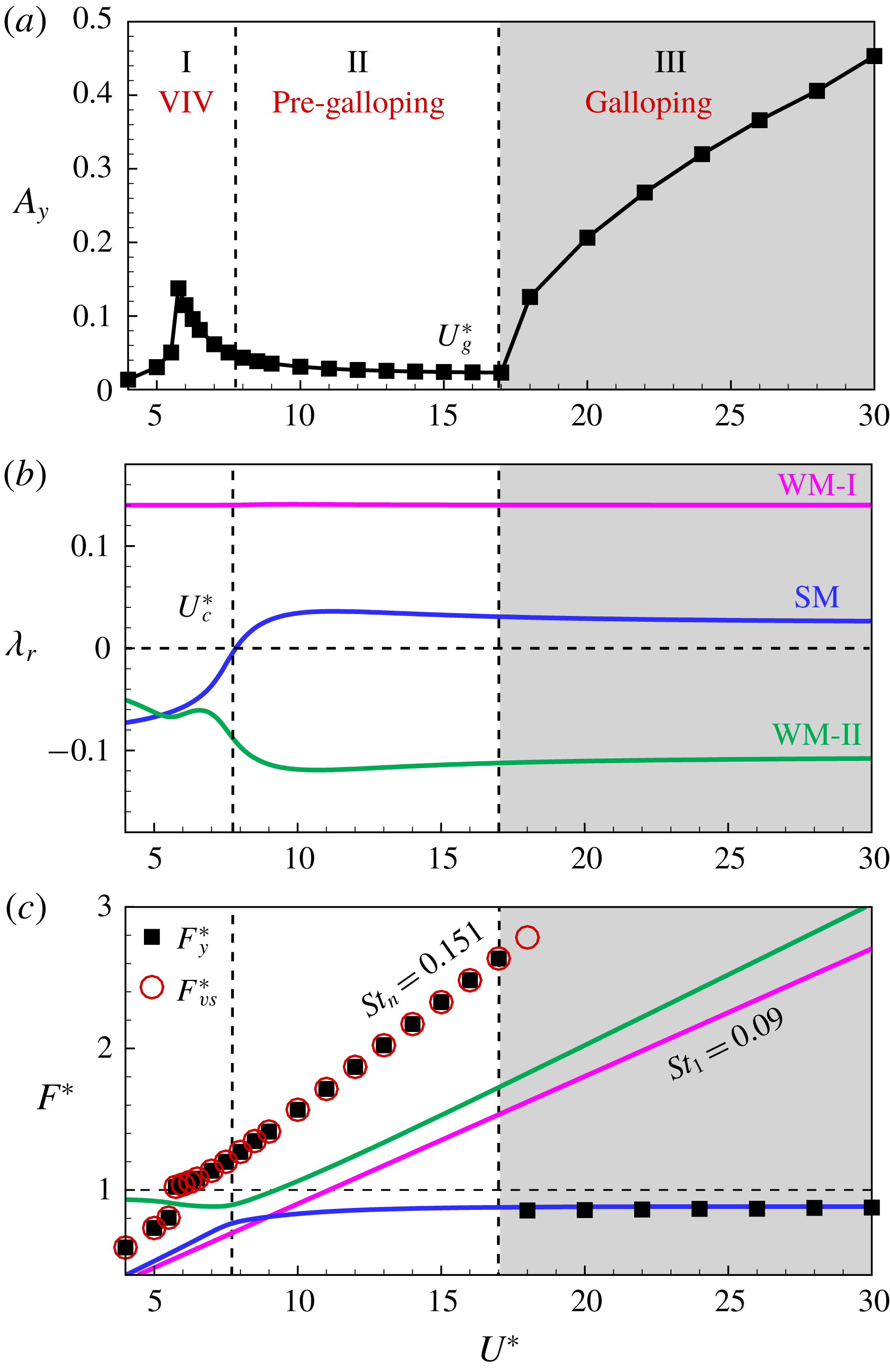
Figure 17. Flow-induced vibration of a square cylinder at $(Re,m^{\ast })=(150,10)$ : (a) transverse vibration amplitude obtained from CFD/CSD simulations, (b) growth rates and (c) eigenfrequencies of the leading three unstable modes obtained from LSA. The dominant vibration frequency (black solid squares) and vortex-shedding frequency (red hollow circles) in the saturated state obtained from CFD/CSD simulations are also plotted in (c) for comparison. The frequencies are normalized by the reduced natural frequency of the structure  $F_{s}$ .

To verify this conjecture, a comparative study between the results from LSA and CFD/CSD simulations is conducted; $(Re,m^{\ast })=(150,10)$ is selected as a representative case to explore the inherent dynamics of galloping. Figure 17(a) illustrates the vibration amplitude of the square cylinder obtained from numerical simulations; figure 17(b,c) presents the growth rates and eigenfrequencies of the leading unstable modes analysed by LSA, as a function of  $U^{\ast }$ . The vibration frequency of the cylinder and the vortex-shedding frequency in the nonlinear saturation state obtained from CFD/CSD simulations are also plotted in figure 17(c) for comparison. The frequencies are all normalized by the structural natural frequency  $F_{s}$ . As can be seen, the response range can be divided into three regimes (marked by I, II and III in the figure) by two critical reduced velocities, i.e. the instability onset of SM ( $U_{c}^{\ast }$ ) obtained from LSA and the critical threshold of galloping ( $U_{g}^{\ast }$ ) acquired from direct numerical simulations. The FIV responses corresponding to the three regimes are VIV, pre-galloping and galloping, respectively. In essence, the pre-galloping regime also belongs to VIV. As will be discussed later, we use the term ‘pre-galloping’ primarily to denote the regime where the SM is unstable but galloping does not occur.

In regime I, only the leading fluid mode WM-I is unstable, the response of the coupled system is dominated by vortex-excited resonance and no coupled-mode flutter occurs, which is consistent with the LSA results of Yao & Jaiman (Reference Yao and Jaiman2017). As a consequence, the square cylinder only shows large-amplitude vibrations in a quite narrow lock-in region. During lock-in, the vibration frequency as well as the vortex-shedding frequency is synchronized with the structural natural frequency. Outside the lock-in region, both the cylinder vibration frequency and the vortex-shedding frequency coincide with the vortex shedding frequency of a stationary square cylinder. The response behaves as a forced vibration under the effect of unsteady vortex shedding. It is worth noting that the eigenfrequency of WM-I ( $F_{WM-I}=St_{l}=0.09$ ) deviates substantially from the nonlinear vortex-shedding frequency ( $St_{n}=0.151$ ), as shown in figure 17(c). This is because the linear model can only predict the characteristic frequency of the wake in the vicinity of the critical $Re$ , but fails to capture the frequency for $Re$ far away from the critical point, where the vortex-shedding frequency is strongly modulated by nonlinear effects (Barkley Reference Barkley2006). For the present case, the selected $Re=150$ is far from the critical Reynolds number of a square cylinder $Re_{cr}=45.2$ .

In regime III, both the WM-I and SM are unstable. It is well known that the instability of SM is an important feature of flutter, and flutter often leads to larger vibration amplitude of the structure than that induced by vortex-excited resonance (Zhang et al. Reference Zhang, Li, Ye and Jiang2015a ). As expected, the vibration amplitude of the cylinder increases monotonically with increasing $U^{\ast }$ in this regime. Very importantly, the dominant vibration frequency of the square cylinder exactly matches the eigenfrequency of SM during the galloping, as demonstrated in figure 17(c). This confirms that the instability of SM is the primary cause of galloping-type oscillation. In other words, the instability of SM is a necessary condition for the occurrence of galloping. On the other hand, the dominant frequency of vortex shedding still follows the Strouhal law and is close to the vortex shedding frequency of a fixed square cylinder with a value of 0.151. The variation trend of vortex-shedding frequency ratio is qualitatively consistent with that of WM-I with regard to  $U^{\ast }$ . Thus, it can be inferred that the high-frequency vortex shedding in the cylinder wake is induced by the leading fluid mode WM-I. As discussed previously, the essential nature of decoupling between the low-frequency vibration and the high-frequency vortex shedding during galloping is owing to the weak coupling between SM and WM-I.

In regime II, the SM is also unstable. However, numerical simulation results indicate that the FIV response in this regime is still dominated by VIV with no galloping-type oscillation. As can be seen from figure 17, the critical reduced velocity of galloping predicted by LSA ( $U_{c}^{\ast }=7.85$ ) is much lower than that calculated by direct CFD/CSD simulation method ( $U_{g}^{\ast }=17.0$ ). This means that the linear dynamic model significantly underestimates the onset reduced velocity of galloping. In the next section, we try to reveal the fundamental reason for this discrepancy from the perspective of nonlinear competition between the SM and the leading fluid mode WM-I.

5.3 Mode competition mechanism

Two important and interesting questions arise from the former results: for the case of more than one eigenmode being linearly unstable, how do the unstable modes interact with each other? And which one will dominate the final response?

Zhang et al. (Reference Zhang, Li, Ye and Jiang2015a ) investigated the underlying mechanism of VIV lock-in through LSA and direct numerical simulation. They reported that in the flutter-induced lock-in region, the SM and WM are both unstable, and the essential characteristic of flutter is the competition between the two unstable modes. It was found that, in the initial development stage of numerical simulation, the two modes co-exist. However, as the vibration amplitude increases, the SM gradually dominates the dynamics of the coupled system and locks the WM, causing the vortex-shedding frequency to be locked onto the structural natural frequency.

Inspired by previous work, in this section, we attempt to uncover the interaction mechanism between SM and WM-I by means of direct numerical simulations. To study the evolution and development of the unstable modes (SM and WM-I), the simulations were initiated from the equilibrium state (steady-state base flow with zero displacement and zero velocity of the cylinder). In this way, we can acquire more dynamical information of the coupled system, especially for the mode competition process.

Figure 18. (a) Evolution process of the transverse displacement $Y$ of the square cylinder with time for $(Re,m^{\ast })=(150,10)$ at $U^{\ast }=10$ . (b,c) Illustrate the PSD results at different time stages. The simulation is initiated from the equilibrium steady state.

Figures 18 and 20 show the representative time histories of cylinder displacement for regimes II and III, respectively, as well as the corresponding PSD results at different time stages. The case of $U^{\ast }=10$ belongs to regime II (pre-galloping) while the case of $U^{\ast }=20$ belongs to regime III (galloping). As can be seen, for $U^{\ast }=10$ , in the initial stage of development $200<t<340$ , the response amplitude does not increase exponentially, but exhibits uneven features, which indicates that there are multiple frequency components at this stage. This is evident from the PSD analysis result shown in figure 18(b), wherein the spectrum has two peak frequencies corresponding to WM-I and SM, respectively. Therefore, it confirms the LSA results: both the WM-I and SM are linearly unstable in regime II. However, as time goes on, WM-I quickly reaches the nonlinear saturation state, and the wake flow is gradually dominated by nonlinear dynamics. In the nonlinear stage, rigorous competition between WM-I and SM is observed because the frequencies of the two unstable modes are very close to each other ( $F_{WM-I}/F_{SM}=1.08$ ). As a result, the SM is locked by the WM-I during the nonlinear mode competition. It can be seen from figure 18 that, over time, the SM gradually disappears and the response is ultimately dominated by WM-I. The process of mode competition is more clearly shown in figure 19 where the time–frequency spectrum of the cylinder displacement is presented. The time–frequency spectrum is achieved using continuous wavelet transforms (CWT), which can provide an insight into the temporal evolution of the frequency content (Zhao et al. Reference Zhao, Nemes, Jacono and Sheridan2018). In this work, the Morlet wavelet was employed for CWT analysis. As can be seen, in the linear stage, the intensity of both unstable modes increases gradually with time. However, when the nonlinearity occurs the intensity of SM progressively decreases and eventually disappears during the competition with WM-I. The above analysis explains why galloping is not observed in regime II even though the SM is unstable.

Figure 19. Time–frequency spectrum of the transverse displacement based on CWT for $(Re,m^{\ast })=(150,10)$ at $U^{\ast }=10$ .

Figure 20. (a) Evolution process of the transverse displacement $Y$ of the square cylinder with time for $(Re,m^{\ast })=(150,10)$ at $U^{\ast }=20$ . (b–d) Illustrate the PSD results at different time stages. The simulation is initiated from the equilibrium steady state.

This kind of mode lock-in is different from the one observed in coupled-mode flutter of VIV reported in Zhang et al. (Reference Zhang, Li, Ye and Jiang2015a ). For coupled-mode flutter, the WM and SM are both unstable and their eigenfrequencies are also very close ( $0.75<F_{WM}/F_{SM}<0.95$ ). But, eventually, it is the SM that locks the WM in the nonlinear competition, resulting in the classical frequency lock-in phenomenon. However, for the present case in the pre-galloping region ( $1.06<F_{WM-I}/F_{SM}<1.75$ ), it is the leading fluid mode WM-I that wins the competition and finally locks the SM. Consequently, the structure response in regime II exhibits as vortex-excited forced vibration and the galloping-type oscillation is suppressed. In other words, the onset $U^{\ast }$ of galloping is postponed. Table 2 compares the two mode lock-in phenomena and summarizes the underlying physical principles. As can be seen, for both cases, it is the higher-frequency mode that finally wins the competition. Navrose & Mittal (Reference Mittal2016) examined the mode lock-in phenomenon from the energy transfer viewpoint. They showed that the energy transfer coefficient of SM is larger than that of WM in the flutter regime of VIV. As a result, the SM ultimately drives the response of the coupled system towards lock-in.

Table 2. Phenomenon and principle for mode competition in flutter of VIV of a circular cylinder (Zhang et al. Reference Zhang, Li, Ye and Jiang2015a ) and in pre-galloping of a square cylinder (present study). For both cases, the mode with higher frequency finally wins the competition.

To gain more quantitative insight into the mode competition mechanism, we estimated the energy transfer coefficients $E_{c}$ of the leading unstable modes by the ROM-based FSI model (see the derivation in appendix A). The energy transfer coefficient denotes the non-dimensional energy transfer over one period of cylinder oscillation from the fluid to the structure that excludes the exponential growth/decay. It is a function of $(m^{\ast },\unicode[STIX]{x1D706})$ and can be written as

(5.1) $$\begin{eqnarray}E_{c}=2\unicode[STIX]{x03C0}^{2}{\hat{Y}}^{2}m^{\ast }\unicode[STIX]{x1D706}_{r}\unicode[STIX]{x1D706}_{i},\end{eqnarray}$$

where ${\hat{Y}}$ represents the magnitude of the eigenmode for the structural part. The expression shows that the sign of $E_{c}$ is determined by the sign of the real part of eigenvalue ( $\unicode[STIX]{x1D706}_{r}$ ). Therefore, $E_{c}$ is positive for unstable modes while negative for stable modes. It is also noted that $E_{c}$ is directly proportional to the real and imaginary parts of the eigenmode. This means that the mode with larger growth rate and higher frequency is generally associated with a larger energy transfer coefficient. Figure 22 shows the energy transfer coefficients of the three leading modes as a function of $U^{\ast }$ for $(Re,m^{\ast })=(150,10)$ . It can be seen that $E_{c}$ of WM-I is always larger than that of SM in the whole unstable region. Thus, WM-I is expected to dominate the temporal evolution of cylinder displacement in the pre-galloping region when strong mode competition occurs.

For the case of a larger reduced velocity $U^{\ast }=20$ (figure 20), since the frequency of SM departs too far from that of WM-I ( $F_{WM-I}/F_{SM}=2.04$ ), the competition between the two unstable modes becomes weaker and no mode lock-in can happen. As a result, the two modes coexist all the time and act in a nearly decoupled manner to contribute to the response of the fluid–structure system. Because the growth rate of WM-I is much larger than that of SM (figure 17 b), the developing process of galloping contains two interesting stages, as illustrated in figure 20(a). In the first stage, WM-I develops rapidly and quickly reaches the nonlinear saturation state. At this time stage, the contribution of SM to the coupled system is very weak and has not been clearly reflected in the response. The second stage of growth in the vibration amplitude is contributed by SM. For that the growth rate of SM is quite small, the response takes a very long time to reach the final nonlinear saturation state (quasi-periodic oscillation state). Figure 21 presents the time–frequency spectrum of the cylinder displacement for $U^{\ast }=20$ . As can be seen, during the entire development process, the frequency spectrum contains two distinct frequency components, corresponding to WM-I and SM, respectively. It is worth noting that an intermediate frequency $F\approx 0.07$ appears when $t>3000$ . The peak power spectrum of this frequency is nearly two orders lower than those of WM-I and SM. Moreover, it has a close relation with the frequencies of WM-I and SM in the saturated state, i.e. $F\approx F_{WM-I}-2F_{SM}$ . Hence, the appearance of this frequency component is the result of the nonlinear interaction between the fluid mode and the structure mode.

Figure 21. Time–frequency spectrum of the transverse displacement based on CWT for $(Re,m^{\ast })=(150,10)$ at $U^{\ast }=20$ .

Figure 22. Variation of energy transfer coefficients of the three leading modes with $U^{\ast }$ for $(Re,m^{\ast })=(150,10)$ .

To further verify the correctness of the linear model, the growth rates of the unstable modes predicted by LSA are compared with those measured from the time histories of the cylinder displacement in the linear stage, as shown in figure 23. The autoregressive moving-averaging approach (Box, Jenkins & Reinsel Reference Box, Jenkins and Reinsel1994) was employed to recover the growth rates from the calculated time-series data. This method has been shown to be able to correctly estimate the damping ratios of fluid–structure interaction systems (Zhu & So Reference Zhu and So2000; McNamara & Friedmann Reference McNamara and Friedmann2007). As can be seen, the results are in good agreement for all $U^{\ast }$ considered, which indicates that the ROM-based FSI model has accurately captured the linear dynamics of the coupled system.

Figure 23. Comparison of the growth rates predicted by LSA and those measured from direct numerical simulations for $(Re,m^{\ast })=(150,10)$ at various  $U^{\ast }$ .

From the above analysis, we know that the instability of SM is the primary cause of the galloping phenomenon. This provides clear evidence that transverse galloping is essentially a kind of single-degree-of-freedom (SDOF) flutter (Nakamura Reference Nakamura1990). As this kind of SDOF flutter occurs at relatively large reduced velocities, the vibration frequency of the structure is far from the natural vortex-shedding frequency (natural vortex-shedding frequency refers to the frequency component which is close to the vortex-shedding frequency of a stationary square cylinder). Hence, the oscillation of the structure is unable to lock the vortex shedding in the wake, resulting in the existence of a high-frequency component in the structure response. Therefore, the high-speed galloping can be understood as a type of SDOF flutter, superimposed by a forced vibration induced by the natural vortex shedding.

5.4 Effect of mass ratio

The numerical study of Joly et al. (Reference Joly, Etienne and Pelletier2012) indicated that when the mass ratio is less than a critical value, the galloping phenomenon will not occur. This interesting phenomenon is also confirmed by the present numerical results, as demonstrated in § 4.1. To determine the critical mass ratio, the variation of oscillation amplitude with $m^{\ast }$ at a large $U^{\ast }=40$ is investigated, as illustrated in figure 24. It can be seen that, with the decrease of  $m^{\ast }$ , the vibration amplitude first gradually decreases ( $m^{\ast }\geqslant 4$ ) and then slightly increases ( $m^{\ast }<4$ ). Therefore, the critical mass ratio is $m_{cg}^{\ast }=4$ , approximately. Below this value galloping completely disappears and the response of the coupled system is dominated by VIV for all $U^{\ast }$ .

Figure 24. Variation of the transverse vibration amplitude with $m^{\ast }$ for $Re=150$ at a sufficiently large $U^{\ast }=40$ .

Figure 25. LSA results for $Re=150$ at various $m^{\ast }$ : (a) root loci of the coupled system; (b,c) present the growth rate and frequency ratio of CM-I, as a function of  $U^{\ast }$ . Note that CM-I resembles the SM in the unstable region.

To further understand this phenomenon, we present the root loci as a function of $U^{\ast }$ for $Re=150$ at various $m^{\ast }$ in figure 25. As can be seen, with the decrease of $m^{\ast }$ , the growth rate of CM-I increases gradually. Note that CM-I exhibits as the SM in the unstable region for all mass ratios. This means that the SM tends to be more unstable at lower  $m^{\ast }$ . However, numerical simulation results show that the galloping-type oscillation completely vanishes at sufficiently low $m^{\ast }$ conditions. As an example, we show the time evolution of cylinder displacement and the corresponding PSD results for $(Re,m^{\ast })=(150,2)$ at a representative $U^{\ast }=40$ in figure 26. Similarly, the simulation was initiated from the unstable steady-state base flow with zero initial displacement and velocity of the cylinder. From figure 26(b), we can see that in the early stage, there exist two unstable modes in the response, namely the SM and the WM-I, which is consistent with the LSA results. The two unstable modes develop rapidly and quickly enter the nonlinear stage. The nonlinear mode competition eventually leads to the mode lock-in of SM by WM-I in the whole unstable region $U^{\ast }>U_{c}^{\ast }$ , resulting in the disappearance of the galloping phenomenon. This is mainly because, although the instability of SM is intensified at low  $m^{\ast }$ , the forced vibration effect induced by the natural vortex shedding is also enhanced when the structure is getting lighter.

Figure 26. (a) Evolution process of the transverse displacement $Y$ of the square cylinder with time for $(Re,m^{\ast })=(150,2)$ at $U^{\ast }=40$ . (b,c) Illustrate the corresponding PSD results at different time stages. The simulation is initiated from the equilibrium steady state.

5.5 Effect of Reynolds number

The Reynolds number has a great influence on the FIV response of a square cylinder. As shown in figure 9, for $m^{\ast }=10$ , galloping starts to occur when $Re>139$ . Below this value, the response is dominated by VIV only. The quasi-steady analyses by Barrero-Gil, Sanz-Andrés & Roura (Reference Barrero-Gil, Sanz-Andrés and Roura2009) and Joly et al. (Reference Joly, Etienne and Pelletier2012) indicated that the $Re$ threshold can be determined by using the Den Hartog criterion. The slope of the vertical force coefficient changes sign when the $Re$ passes though the critical value. In this section, we further investigate the effect of $Re$ on the FIV response of a square cylinder. The intention is to reveal whether mode competition still exists at lower  $Re$ .

Figure 27 shows the root loci of the coupled system for $m^{\ast }=10$ at three typical Reynolds numbers, $Re=80$ , 100 and 120. As can be seen, the SM begins to become unstable at large $U^{\ast }$ when $Re\geqslant 100$ , approximately. However, numerical simulation results suggest that galloping is not observed until $Re>139$ . Apparently, the inconsistency is also due to the mode competition mechanism, as discussed previously. A typical case for $Re=139$ at a large $U^{\ast }=40$ is given in figure 28 to show the mode competition process. Since $Re=139$ is very close to the critical Reynolds number, the SM decays very slowly and takes quite a long time to completely vanish.

Figure 27. Root loci of the coupled system as a function of $U^{\ast }$ for $m^{\ast }=10$ at three representative Reynolds numbers: (a)  $Re=80$ , (b)  $Re=100$ and (c)  $Re=120$ . As can be seen, the SM begins to be unstable at large $U^{\ast }$ when $Re\geqslant 100$ , approximately.

Figure 28. (a) Evolution process of the transverse displacement $Y$ of the square cylinder with time for $(Re,m^{\ast })=(139,10)$ at $U^{\ast }=40$ . (b,c) Illustrate the corresponding PSD results at different time stages. The simulation is initiated from the equilibrium steady state.

Figure 29 shows the neutral stability curve of the SM analysed by LSA and the onset boundary of galloping acquired from direct numerical simulations in the $(Re,U^{\ast })$ plane for $m^{\ast }=10$ . It can be seen that the critical reduced velocity predicted by LSA is generally lower than the onset reduced velocity calculated by CFD/CSD simulation method. The grey shaded region between the two critical boundaries indicates the regime where strong mode competition occurs. In this region, both the SM and WM-I are linearly unstable, but the WM-I locks the SM in the nonlinear stage. As a result, the galloping-type oscillation is suppressed and the response is still dominated by VIV in this region.

Figure 29. Neutral stability curve of the SM obtained from LSA (blue squares) and the galloping onset boundary obtained from direct CFD/CSD simulations (dark circles) for $m^{\ast }=10$ in the $(Re,U^{\ast })$ plane. The plane is divided into three regions: VIV, galloping and pre-galloping (grey shaded).

It should be noted that the critical mass ratio and Reynolds number are determined based on the numerical computations at a large $U^{\ast }=40$ . The critical values may slightly change when the test reduced velocity is further increased.