2.1 Basic Notation and Assumptions

Following Taylor's (Reference Taylor1986, Reference Taylor1987) and Emms et al. (Reference Emms, Haberman and Savoulli2007) approaches, we propose a stochastic, discrete-time premium pricing model to describe a competitive insurance market. Thus, the following notation is needed:

V_k: denotes the volume of business (or exposure) underwritten by the insurer in year [k, k + 1). This volume may be measured in any meaningful unit, e.g. number of claims incurred, total man-hours at risk (for workers’ compensation insurance). In our paper, we consider the number of claims incurred as the volume of exposure.

π_k: denotes the break-even premium in year [k, k + 1), i.e. risk premium plus expenses per unit exposure.

p_k: denotes the premium charged by the insurer in year [k, k + 1). This is our control parameter.

$$\[--><$>{{\bar{p}}_k}:<$><!--\]$$ denotes the “average” premium charged by the market in year [k, k + 1). We further assume that this process is stochastic, see also Emms et al. (Reference Emms, Haberman and Savoulli2007). Let $$\[--><$>\left( {\Omega, {\cal F},{\cal P}} \right)<$><!--\]$$ be the probability space and $$\[--><$>\left\{ {{{{\bar{p}}}_k}|k\: = \:1,2, \ldots } \right\}<$><!--\]$$ be the sequence of random variables defined on this probability space.

r: denotes the rate of return on equity required by shareholders of the insurer whose strategy is under consideration. We further assume that this rate is deterministic.

$$\[--><$>\upsilon <$><!--\]$$ : denotes the corresponding discount factor, $$\[--><$>\upsilon \: = \:{{\left( {1\: + \:r} \right)}^{{\rm{ - }}1}} <$><!--\]$$ .

θ_k: denotes the set of all other stochastic variables (which are assumed to be independently distributed in time and Gaussian) and it is considered to be relevant to the demand function in year [k, k + 1), such as inflation, interest rate, exchange rate, marketing etc. In other words, this stochastic parameter tries to number the contracts that the company loses or gains due to these disturbances, which actually affect the volume of business of the insurance company. However, for the purposes of the present version of the paper, further analysis of the micro and macro economics parameters that get involved in θ_k is omitted. We will leave it as a future direction to our research.

In this paper, as in Emms et al. (Reference Emms, Haberman and Savoulli2007) and Taylor (Reference Taylor1986), we make the following assumptions.

Additionally, extending Taylor's (Reference Taylor1986, Reference Taylor1987) assumptions, we assume that the demand function is stochastic (because of θ_k and $$\[--><$>{{\bar{p}}_k}<$><!--\]$$ ). Here, we denote the wealth process w_k as the insurer's capital at time [k, k + 1), following Emms et al. (Reference Emms, Haberman and Savoulli2007) ideas, so we obtain

$${{w}_{k + 1}}\: = \:{\rm{ - }}{{a}_k}{{w}_k}\: + \:({{p}_k}{\rm{ - }}{{\pi }_k}){{V}_k},$$

where a_k∈[0,1] denotes the excess return on capital (i.e. return on capital required by the shareholders of the insurer whose strategy is under consideration). Thus, −a_kw_k is the cost of holding w_k in the time interval [k,k + 1).

Following Taylor (Reference Taylor1986, Reference Taylor1987), the volume of business (or exposure) of an insurance company for a given sequence of average market prices over the k ^th year is given by a relation of the following type

$${{V}_k}\:{\triangleq}\:{{f}_k}\left( {{{V}_{k{\rm{ - }}1}},{{p}_k},{{{\bar{p}}}_k},{{\theta }_k}} \right),$$

where p_k is the controller and θ_k denotes the set of all other random variables (disturbances) which are considered to be relevant to the demand function. Under this assumption V_k is a stochastic variable and depends on k.

Our aim is to determine the strategy which maximizes the expected total utility of the wealth at time k over a finite time horizon T. As it has been also considered by Emms et al. (Reference Emms, Haberman and Savoulli2007), we use a linear discounted function (of wealth).

Analytically, we want to maximize

$${\mathop{{\max }}\limits_{{{{p}_k}}}} \,{\Bbb E}\left[ {\mathop{\sum}\limits_{k\: = \:0}^T {U({{w}_k},k)} } \right],$$

where $$\[--><$>U({{w}_k},k) = {{\upsilon }^k} {{w}_k}<$><!--\]$$ is the present value of the wealth w_k.

Consequently, substituting (2.2) into (2.1), the wealth process w_k is given by (2.4)

$${{w}_{k\: + \:1}}\: = \:{\rm{ - }}{{a}_k}{{w}_k}\: + \:({{p}_k}{\rm{ - }}{{\pi }_k}){{f}_k}({{V}_{k{\rm{ - }}1}},{{p}_k},{{\bar{p}}_k},{{\theta }_k}),$$

and w ₀, V ₀, V ₋₁ (the volume of business now and for the previous year) a ₀ and π ₀ are the initial conditions.

Extending Taylor's (Reference Taylor1986, Reference Taylor1987) ideas, who assumed that the volume of business in year k+1 is proportional to the demand of the preceding year, in this paper we propose that the volume of business is proportional to the average premium charged by the market (see Assumption 3), but reverse proportional to the premium rate charged by the insurer in year k. Empirically speaking, this new approach might be considered as a little more realistic, since it is true that whenever the average premium stays unchanged and the premium charged by the insurer increases, unavoidably the company's volume of business might decrease. On the other hand, whenever the premium calculated by the insurer stays unchanged and the average premium decreases, the volume of business might decrease as well. These thoughts lead to the assumption that the volume of business should be proportional to the rate $$\[--><$>\frac{{{{{\bar{p}}}_k}}}{{{{p}_k}}}<$><!--\]$$ .

Additionally, it is realistic to assume that there might be an unexpected set of parameters, which can modify (i.e. decrease or increase) the volume of business. Consequently, we can assume that this set of parameters can be modelled using the stochastic variable θ_k, which can take either positive or negative values. In this paper, since we are more interested in investigating the premium strategy of an insurance company when it is expected to lose part of the market, we assume that the expected values of θ_k is positive (i.e. $$\[--><$>{\Bbb E}\left( {{{\theta }_k}} \right)\, \gt \,\mu <$><!--\]$$ , where μ > 0 is a deductible parameter which can be pre-defined by the managerial team), and then the volume of business is strictly decreasing, i.e. losing part of the competitive market. Obviously, within the next lines, the case $$\[--><$>{\Bbb E}\left( {{{\theta }_k}} \right)\, \lt \,\mu <$><!--\]$$ is also discussed, however this case is not very interested since it implies that the insurance company is increasing gradually its volume, and any change in its premium policy might affect it negatively.

Consequently, we can assume that the volume of business is given by

$${{V}_k}\: = \:{{V}_{k{\rm{ - }}1}}\frac{{{{{\bar{p}}}_k}}}{{{{p}_k}}}{\rm{ - }}{{\theta }_k},$$

where θ_k is being involved as an additive white noise.

2.2 Calculation of the Optimal Premium

After the basic notations, and the mathematical formulation of the problem, we need to calculate the optimal premium, which maximize the expected total utility of the wealth (2.3).

Following the general ideas about stochastic dynamic programming and control theory in a discrete-time framework, see for instance the classical books by Bertzekas (Reference Bertzekas2000) and Kushner (Reference Kushner1970), we determine the strategy which maximises the expected total utility of wealth (2.3) over a finite time horizon T, and over a choice of strategies p. This is similar to the objective function used by Taylor (Reference Taylor1986, Reference Taylor1987), and Emms et al. (Reference Emms, Haberman and Savoulli2007).

The next Theorem provides us with the optimal premium strategy for the finite time horizon maximization problem (2.3)–(2.5), see also Jacobson (Reference Jacobson1974) and Kushner (Reference Kushner1970).

$${{w}_{k\: + \:1}}\: = \:{\rm{ - }}{{a}_k}{{w}_k}\: + \:({{p}_k}{\rm{ - }}{{\pi }_k})\left( {{{V}_{k{\rm{ - }}1}}\frac{{{{{\bar{p}}}_k}}}{{{{p}_k}}}{\rm{ - }}{{\theta }_k}} \right),$$

where $$\[--><$>{\Bbb E}\left( {{{\theta }_k}} \right)\, \gt \,\mu <$><!--\]$$ , μ > 0, and for the maximization problem defined by

$${\mathop{{\max }}\limits_{{{{p}_k}}}} \,{\Bbb E}\left[ {\mathop{\sum}\limits_{i\: = \:k}^{T{\rm{ - }}1} {{{\upsilon }^i} {{w}_i}} } \right],$$

with initial conditions w ₀, V ₀, V ₋₁, a ₀, and π ₀, the optimal strategy process $$\[--><$>p_{k}^{\ast} <$><!--\]$$ is given by

$$ p_{k}^{\ast} \: = \:{{\left( {\frac{1}{{{\Bbb E}\left( {{{\theta }_k}} \right)}}{{\pi }_k}{{V}_{k{\rm{ - }}1}}{\Bbb E}({{{\bar{p}}}_k})} \right)}^{1/2}} \ {{for}} \ k\: = \:0,1, \ldots, T{\rm{ - }}1, $$

where $$\[--><$>{{\bar{p}}_k} <$><!--\]$$ , π_k is the “average” and the break-even premium respectively, in year k;V_{k −1}is the volume of exposure underwritten by the insurer in year k−1, and $$\[--><$>{\Bbb E}\left( {{{\theta }_k}} \right)<$><!--\]$$ is the expectation of the (stochastic) disturbance θ_k in year k, and the maximum value of (2.7) is given by

$${{w}_0}{{d}_0}\: + \:{{e}_0}.$$

Moreover, we define

$${{d}_k}\: = \:{{\upsilon }^k} {\rm{ - }}{{a}_k}{{d}_{k\: + \:1}}\: \gt \:0\,, \ {{and}} \ {{d}_T}\: = \:0,$$

$$ no{\quad \qquad {{e}_k}\: = \: {\rm{ - }}{{d}_{k\: + \:1}}\left( {{{{\left( {\frac{1}{{{\Bbb E}\left( {{{\theta }_k}} \right)}}{{\pi }_k}{{V}_{k{\rm{ - }}1}}{\Bbb E}({{{\bar{p}}}_k})} \right)}}^{1/2}} {\Bbb E}\left( {{{\theta }_k}} \right){\rm{ - }}{{V}_{k{\rm{ - }}1}}{\Bbb E}\left( {{{{\bar{p}}}_k}} \right)} \right) \cr & \quad\: + \:{{d}_{k\: + \:1}}{{\pi }_k}\left( {{\Bbb E}\left( {{{\theta }_k}} \right){\rm{ - }}{{V}_{k{\rm{ - }}1}}{\Bbb E}\left( {{{{\bar{p}}}_k}} \right){{{\left( {\frac{1}{{{\Bbb E}\left( {{{\theta }_k}} \right)}}{{\pi }_k}{{V}_{k{\rm{ - }}1}}{\Bbb E}({{{\bar{p}}}_k})} \right)}}^{{\rm{ - }}1/2}} } \right)\: + \:{{e}_{k\: + \:1}}\,,\ {{and}} \ {{e}_T}\: = \:0. $$

Proof Define

$${{J}_k}({{w}_k})\:{\triangleq}\:{\mathop{{\max }}\limits_{{{{p}_k},{{p}_{k\: + \:1}}, \ldots, {{p}_{T{\rm{ - }}1}}}}} {{{\Bbb E}}_{|{{w}_k}}}\left[ {\mathop{\sum}\limits_{i\: = \:k}^{T{\rm{ - }}1} {{{\upsilon }^i} {{w}_i}} } \right].$$

Then, as it is known [6], the optimal performance criterion satisfied the Bellman equation

$$no{ \qquad \qquad \qquad \qquad \qquad \quad {{J}_k}({{w}_k}) = {\mathop{{\max }}\limits_{{{{p}_k}}}} \,{{{\Bbb E}}_{|{{w}_k}}}\left\{ {{{\upsilon }^k} {{w}_k}\: + \:{{J}_{k\: + \:1}}({{w}_{k\: + \:1}})} \right\} \cr = {\mathop{{\max }}\limits_{{{{p}_k}}}} \left\{ {{{\upsilon }^k} {{w}_k}\: + \:{{{\Bbb E}}_{|{{w}_k}}}{{J}_{k\: + \:1}}({{w}_{k\: + \:1}})} \right\} $$

where $$\[--><$>{{{\Bbb E}}_{|{{w}_k}}}\left( {{{{\bar{p}}}_k}} \right)\: = \:{\Bbb E}\left( {{{{\bar{p}}}_k}} \right) <$><!--\]$$ and $$\[--><$>{{{\Bbb E}}_{|{{w}_k}}}\left( {{{\theta }_k}} \right)\: = \:{\Bbb E}\left( {{{\theta }_k}} \right)\: \gt \:\mu \: \gt \:0 <$><!--\]$$ , and $$\[--><$>J{\pre}_{T}({{w}_T})\: = \:{{w}_T}{{d}_T}\: + \:{{e}_T}\: = \:0 <$><!--\]$$ ; see (2.10), and (2.11).

We now show by induction that

$$ {{J}_k}({{w}_k})\: = \:{{w}_k}{{d}_k}\: + \:{{e}_k} $$

solves (2.13) by noting that (2.14) is true for k = T by assuming that (2.14) is true for k+1 and by proving is true for k. Substituting the assumed expression for J_{k + 1}(w_{k + 1}) into the right hand side (2.13) we obtain

$$ {{J}_k}({{w}_k})\: = \:{\mathop{{\max }}\limits_{{{{p}_k}}}} \left\{ {{{\upsilon }^k} {{w}_k}\: + \:{{{\Bbb E}}_{|{{w}_k}}}{{J}_{k\: + \:1}}({{w}_{k\: + \:1}})} \right\}\: = \:{\mathop{{\max }}\limits_{{{{p}_k}}}} \left\{ {{{\upsilon }^k} {{w}_k}\: + \:{{{\Bbb E}}_{|{{w}_k}}}({{w}_{k\: + \:1}}){{d}_{k\: + \:1}}\: + \:{{e}_{k\: + \:1}}} \right\}, $$

and from (2.6) we have

$$ no{ {\mathop{{\max }}\limits_{{{{p}_k}}}} \left\{ {{{\upsilon }^k} {{w}_k}\: + \:{{{\Bbb E}}_{|{{w}_k}}}\left[ {{\rm{ - }}{{a}_k}{{w}_k}\: + \:\left( {{{p}_k}{\rm{ - }}{{\pi }_k}} \right){{V}_k}} \right]{{d}_{k\: + \:1}}\: + \:{{e}_{k\: + \:1}}} \right\} \cr \quad= \mathop {\max }\limits_{{{p}_k}} \left\{ {{{\upsilon }^k} {{w}_k}{\rm{ - }}{{a}_k}{{w}_k}{{d}_{k\: + \:1}} + {{d}_{k\: + \:1}}({{p}_k}{\rm{ - }}{{\pi }_k})\left. {\left( {{{V}_{k{\rm{ - }}1}}\frac{{{\Bbb E}\left( {{{{\bar{p}}}_k}} \right)}}{{{{p}_k}}}{\rm{ - }}{\Bbb E}\left( {{{\theta }_k}} \right)} \right)} \right]\: + \:{{e}_{k\: + \:1}}} \right\} \cr \quad= \mathop {\max }\limits_{{{p}_k}} \left\{ {{{\upsilon }^k} {{w}_k}{\rm{ - }}{{a}_k}{{w}_k}{{d}_{k\: + \:1}}{\rm{ - }}{{d}_{k\: + \:1}}\left( {{{p}_k}{\Bbb E}\left( {{{\theta }_k}} \right){\rm{ - }}{{V}_{k{\rm{ - }}1}}{\Bbb E}\left( {{{{\bar{p}}}_k}} \right)} \right)\: + \:{{d}_{k\: + \:1}}{{\pi }_k}\left( {{\Bbb E}\left( {{{\theta }_k}} \right){\rm{ - }}{{V}_{k{\rm{ - }}1}}\frac{{{\Bbb E}\left( {{{{\bar{p}}}_k}} \right)}}{{{{p}_k}}}} \right)\: + \:{{e}_{k\: + \:1}}} \right\} \cr \quad= \mathop {\max }\limits_{{{p}_k}} \left\{ {{\rm{ - }}{{w}_k}({{a}_k}{{d}_{k\: + \:1}}{\rm{ - }}{{\upsilon }^k} ){\rm{ - }}{{d}_{k\: + \:1}}\left( {{{p}_k}{\Bbb E}\left( {{{\theta }_k}} \right){\rm{ - }}{{V}_{k{\rm{ - }}1}}{\Bbb E}\left( {{{{\bar{p}}}_k}} \right)} \right)\: + \:{{d}_{k\: + \:1}}{{\pi }_k}\left( {{\Bbb E}\left( {{{\theta }_k}} \right){\rm{ - }}{{V}_{k{\rm{ - }}1}}\frac{{{\Bbb E}\left( {{{{\bar{p}}}_k}} \right)}}{{{{p}_k}}}} \right)\: + \:{{e}_{k\: + \:1}}} \right\}. \cr$$

The controller that maximizes the above expression, (2.15), is given by (2.8), since

$$ A\: = \:{{w}_k}\left( {{{\upsilon }^k} {\rm{ - }}{{a}_k}{{d}_{k\: + \:1}}} \right)\: + \:\left( {{{V}_{k{\rm{ - }}1}}{\Bbb E}\left( {{{{\bar{p}}}_k}} \right){\rm{ - }}{{p}_k}{\Bbb E}\left( {{{\theta }_k}} \right)} \right){{d}_{k\: + \:1}}{\rm{ - }}{{d}_{k\: + \:1}}{{\pi }_k}\left( {{{V}_{k{\rm{ - }}1}}\frac{{{\Bbb E}\left( {{{{\bar{p}}}_k}} \right)}}{{{{p}_k}}}{\rm{ - }}{\Bbb E}\left( {{{\theta }_k}} \right)} \right)\: + \:{{e}_{k\: + \:1}}. $$

The first derivative of A with respect to p_k is given

$$ \frac{{\partial A}}{{\partial {{p}_k}}}\: = \:{{d}_{k\: + \:1}}{{\pi }_k}{{V}_{k{\rm{ - }}1}}\frac{{{\Bbb E}\left( {{{{\bar{p}}}_k}} \right)}}{{p_{k}^{2} }}{\rm{ - }}{{d}_{k\: + \:1}}{\Bbb E}\left( {{{\theta }_k}} \right)\: = \:{{d}_{k\: + \:1}}\left( {{{\pi }_k}{{V}_{k{\rm{ - }}1}}\frac{{{\Bbb E}\left( {{{{\bar{p}}}_k}} \right)}}{{p_{k}^{2} }}{\rm{ - }}{\Bbb E}\left( {{{\theta }_k}} \right)} \right). $$

If we equalize the first derivative with zero, i.e. $$\[--><$>\frac{{\partial A}}{{\partial {{p}_k}}}\: = \:0 <$><!--\]$$ , we obtain

$$ {{d}_{k\: + \:1}}\left( {{{\pi }_k}{{V}_{k{\rm{ - }}1}}\frac{{{\Bbb E}\left( {{{{\bar{p}}}_k}} \right)}}{{p_{k}^{2} }}{\rm{ - }}{\Bbb E}\left( {{{\theta }_k}} \right)} \right)\: = \:0{\mathop{ \Leftrightarrow }\limits^{{{{d}_{k + 1}}\: \ne \:0,\,{}{\Bbb E}\left( {{{\theta }_k}} \right)\: \gt \:\mu \: \gt \:0}}} \;{{\pi }_k}{{V}_{k{\rm{ - }}1}}\frac{{{\Bbb E}\left( {{{{\bar{p}}}_k}} \right)}}{{p_{k}^{2} }}{\rm{ - }}{\Bbb E}\left( {{{\theta }_k}} \right)\: = \:0. $$

The above expression gives the optimal strategy (2.8) as

$$ \frac{{\partial A}}{{{{\partial }^2} {{p}_k}}}\: = \:{\rm{ - }}2{{\pi }_k}{{V}_{k{\rm{ - }}1}}{\Bbb E}({{\bar{p}}_k}){{d}_{k\: + \:1}}\frac{1}{{p_{k}^{3} }}\: \lt \:0, $$

where $$\[--><$>{{\pi }_k},{{V}_{k{\rm{ - }}1}},{\Bbb E}(\overline{{{{p}_k}}} ),\frac{1}{{p_{k}^{3} }} <$><!--\]$$ and $$\[--><$>{{d}_{k\: + \:1}}\: \gt \:0 <$><!--\]$$ .

Now, let's substitute the above into (2.15), we obtain

$${ {\rm{ - }}{{w}_k}({{a}_k}{{d}_{k\: + \:1}}{\rm{ - }}{{\upsilon }^k} ){\rm{ - }}{{d}_{k\: + \:1}} \left( {{{{\left( {\frac{1}{{{\Bbb E}\left( {{{\theta }_k}} \right)}}{{\pi }_k}{{V}_{k{\rm{ - }}1}}{\Bbb E}({{{\bar{p}}}_k})} \right)}}^{1/2}} {\Bbb E}\left( {{{\theta }_k}} \right){\rm{ - }}{{V}_{k{\rm{ - }}1}}{\Bbb E}\left( {{{{\bar{p}}}_k}} \right)} \right) \cr & \qquad+ {{d}_{k\: + \:1}}{{\pi }_k}\left( {{\Bbb E}\left( {{{\theta }_k}} \right){\rm{ - }}{{V}_{k{\rm{ - }}1}}{{{\left( {\frac{1}{{{\Bbb E}\left( {{{\theta }_k}} \right)}}{{\pi }_k}{{V}_{k{\rm{ - }}1}}{\Bbb E}({{{\bar{p}}}_k})} \right)}}^{{\rm{ - }}1/2}} } \right)\: + \:{{e}_{k\: + \:1}}. \cr} $$

Substituting (2.10) and (2.11) in the above expression yields the fact that (2.14) is true. Thus, the proof of the Theorem 1 by induction is complete. □

The following proposition considers the case where the volume of business changes either above or below μ > 0 (i.e., for decreasing or increasing the volume of business above or below the required level, respectively).

$${\Bbb E}(w_{{k\: + \:1}}^{\ast} )\: = \:{{V}_{k{\rm{ - }}1}}{\Bbb E}({{\bar{p}}_k})\: + \:{{\pi }_k}{\Bbb E}({{\theta }_k}){\rm{ - }}\left\{ {{{a}_k}{{w}_k}\: + \:2{{{\left( {{\Bbb E}({{\theta }_k}){{\pi }_k}{{V}_{k{\rm{ - }}1}}{\Bbb E}\left( {{{{\bar{p}}}_k}} \right)} \right)}}^{1/2}} } \right\} \ for \ {\Bbb E}\left( {{{\theta }_k}} \right)\: \gt \:\mu .$$

As Taylor (Reference Taylor1986, Reference Taylor1987), and Emms et al. (Reference Emms, Haberman and Savoulli2007) propose, and in order to take benefit of the analytical formula derived by Theorem 1 for the determination of the premium strategies into a competitive environment, in the next section we use data from the Greek automobile insurance industry, see also the tables of the Hellenic Association of Insurance Companies (2010). Moreover, we assume that the premium strategies concern the price of a contract which refers to a six-month insurance for a car that is 1400cc, 10 years old and its value estimated at 5.000€.

3.1 Premium strategy I: Considering the Entire Market

In the first premium strategy, the expected average premium is calculated considering all the competitors of the market, and their proportions regarding the volume of business. In mathematical terms the expected average premium of the market can be estimated by

$${\Bbb E}\left( {\bar{p}} \right)\: = \:\frac{1}{m}\mathop{\sum}\limits_{i\: = \:1}^K {{{b}_{i,n}}{{p}_{i,n}}}, $$

where $$\[--><$>{{b}_{i,n}}\: = \:{{V}_{i,n}}{{\left( {\mathop{\sum}\nolimits_{i\: = \:1}^K {{{V}_{i,n}}} } \right)}^{{\rm{ - }}1}} <$><!--\]$$ and $$\[--><$>\mathop{\sum}\nolimits_{i\: = \:1}^K {{{b}_{i,n}}} \: = \:1<$><!--\]$$ for every year n, p_{i ,n} is the premium of the company i ^th for the year n; K is the number of the competitors (including also our company's premium) in the insurance market and m is the number of years for the available data (i.e. we assume that we have the uniform distribution for the weight of every year). Moreover, for the calculation of the expected values of the premium of each company and the average market premium respectively, we use the available Greek data, see next paragraphs.

$$p_{k}^{\ast} \: = \:\sqrt {\frac{1}{{m{\Bbb E}\left( {{{\theta }_k}} \right)}}{{\pi }_k}{{V}_{k{\rm{ - }}1}}\mathop{\sum}\limits_{i\: = \:1}^K {{{b}_{i,n}}{{p}_{i,n}}} }, \,{\rm{for}}\,{\Bbb E}\left( {{{\theta }_k}} \right)\: \gt \:\mu \: \gt \:0, \,k\: = \:0,1, \ldots, T{\rm{ - }}1.$$

Proof The proof derives straightforwardly, and it is omitted. □

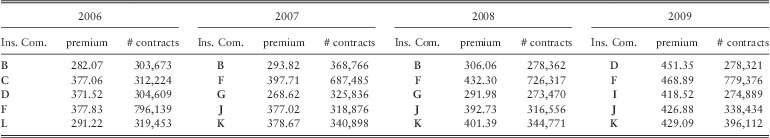
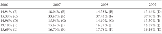
This premium strategy considers the premium and the volume of business of the entire market. The expected average premium of the market is estimated using the (3.1) expression, i.e. as an expected weighted average of each competitor that gets involved in the market. Moreover, it is clear that the premium of the company with the largest volume of business affects most of the market (see also Premium Strategy II). In Table 1, the premium prices and the number of contracts for the 12 major non-life Greek insurance companies for a standard six-month cover of a 10-year old, 1400cc car (with 5.000 Euros covered amount) are presented for the years 2006, 2007, 2008 and 2009.

Table 1 Premium prices in Euros and number of contracts for the 12 major non-life Greek insurance companies, see Hellenic Association of Insurance Companies (2010).

As we can observe in Table 1, and according to the oligopoly theory which began in 1838 with Cournot's oligopoly model, see for more details Friedman (Reference Friedman1983) and the references therein, the Greek non-life insurance industry has an oligopoly market characteristic, since there are only a few main competitors, the insurance products are almost identical (with non-significant differences) and the ownership of the key inputs and barriers imposed by the government. Thus, in the case of oligopolistic market, the revenues of the firms depend on the actions of other competitors as we have considered in our premium strategies; see also Emms et al. (Reference Emms, Haberman and Savoulli2007) and Taylor (Reference Taylor1986, Reference Taylor1987).

According to the premium strategy I, the average premium of the market is equal to the weighted average of the premiums of all the companies involved in the market for every year. Moreover, the volume of business of each company for the years 2006–2009 is presented in Table 2. Finally, Table 3 summarizes the results of the (3.1) expression.

Table 2 (The volume of business, b, in % for the 12 major non-life Greek insurance companies).

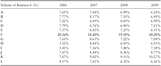
Table 3 (The expected average premium in Euros of the market for the year 2010 is given by $$\[--><$>{\Bbb E}\left( {\bar{p}} \right)\: = \:\frac{1}{m}\mathop{\sum}\nolimits_{i\: = \:1}^K {{{b}_{i,n}}{{p}_{i,n}}} .<$><!--\]$$ ).

As it has already been mentioned above in order to calculate the optimal premium for each company first, we have to estimate the expectation of θ_k which models the set of all other parameters considered to be relevant to the demand function of each company, and the insurance market (i.e. financial environment, managerial policy etc). As it is clear from the relation (2.5) $$\[--><$>{{\hat{\theta }}_k}<$><!--\]$$ (estimation of θ_k) can be calculated by $$\[--><$>{{\hat{\theta }}_k}\: = \:{{V}_{k{\rm{ - }}1}}\frac{{{{{\bar{p}}}_k}}}{{{{p}_k}}}{\rm{ - }}{{V}_k}<$><!--\]$$ .

Thus, considering the above expression, and for the available Greek data we are able to calculate $$\[--><$>{{\hat{\theta }}_k}<$><!--\]$$ for the years 2007, 2008 and 2009 as it is shown at Table 4. So, the expected value of θ_k for the year 2010 can be given by

$${\Bbb E}({{\theta }_k})\: = \:\frac{1}{m}\mathop{\sum}\limits_{i\: = \:1}^m {{{{\hat{\theta }}}_i}} $$

Table 4 (The values of $$\[--><$>{{\hat{\theta }}_k}<$><!--\]$$ , the change in percentage for the volume of business for the years 2007-2009, and the expected values of θ_k for the year 2010).

Then, in Table 4, we present the expected values of θ_k (using the estimations of θ_k). As has been already mentioned before, θ_k denotes the number of contracts that the company loses or gains because of the parameters that affect the volume of business and they have not been included in the model. In our application, the large fluctuations in the expected values of θ_k occur due to a) the limited number of the available data, and b) the impact on each company's volume of business into the market. (Note that since we have available data for only 4 years, it is difficult to provide a good estimation for the expected values of θ_k. However, for the purpose of our application, this drawback is not crucial.)

The values of the stochastic variable θ_k can be either above or below μ > 0. As we have extensively discussed in section 2, we will determine the optimal premium strategy for the year 2010 only for those companies which have positive $$\[--><$>{\Bbb E}({{\theta }_k})\, \gt 0<$><!--\]$$ .

These companies are A, B, E, G and L, see Figure 1.

Figure 1 (The real and the expected volume of business for the 5 Greek insurance companies that have positive $$\[--><$>{\Bbb E}\left( {{{\theta }_k}} \right)\, \gt \,\mu <$><!--\]$$ ).

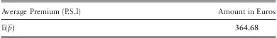
In Table 5, we present the premium for each company for the different values of the break-even premium rate.

Table 5 (The optimal premium strategy in Euros for the 5 Greek insurance companies that have positive $$\[--><$>{\Bbb E}\left( {{{\theta }_k}} \right)<$><!--\]$$ for the different values of the break-even premium rate).

As it is expected, for greater values of the π_k, greater the optimal premium values become. Consequently, since the optimal premium depends on the break-even premium rate, the company should choose its competitive strategy considering the market's construction and its marginal costs; see also Emms et al. (Reference Emms, Haberman and Savoulli2007). Thus, each company should pre-determine its break-even premium rate, in order to calculate the optimal premium strategy which will enlarge its volume of business. The results of Table 5 are shown also at Figure 1.

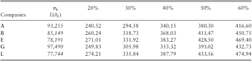
The results of Table 5 (see also Figure 2) are seemingly interesting. For the five insurance companies (A, B, E, G, and L) which expected to experience losses on their volume of business, for a break-even premium rate of 20–30% calculated by the formula 3.2, premiums are below the market average premium of 364.68€. Additionally, it is true that the insurance companies E and L which face similar losses (see Tables 1, 2, and 4) should provide similar premiums, which appear to be the most expensive premiums compared with the premiums of the other 3 companies.

Figure 2 (The optimal premium strategy in Euros for the 5 Greek insurance companies that have positive $$\[--><$>{\Bbb E}\left( {{{\theta }_k}} \right)<$><!--\]$$ for the different values of the break-even premium rate)

At this point, it should be mentioned that in this paper, we are not able to analyze further the results of Table 1, and consequently of Table 5 (and Figure 2), since the analysis of the Greek insurance market, and the micro/macro conditions that get involved for the determination of the premium strategy is far beyond the scopes of the present version of the paper. Additionally, the macro-micro economic analysis of the parameters that affect θ_k is a purpose of future research.

3.2 Premium Strategy II: Following the Leaders of the Market

In this premium strategy, the average premium is calculated considering the premiums of the top K ^top competitors of the market (including the leading company of the market). In mathematical terms the expected average premium of the market is estimated by

$${\Bbb E}\left( {\bar{p}} \right)\: = \:\frac{1}{m}\mathop{\sum}\limits_{i\: = \:1}^{{{K}^{top}} } {b_{{i,n}}^{{top}} p_{{i,n}}^{{top}} }, $$

where $$\[--><$>b_{{i,n}}^{{top}} \: = \:{{V}_{i,n}}{{\left( {\mathop{\sum}\nolimits_{i\: = \:1}^{{{K}^{top}} } {{{V}_{i,n}}} } \right)}^{{\rm{ - }}1}} <$><!--\]$$ and $$\[--><$>\mathop{\sum}\nolimits_{i\: = \:1}^{{{K}^{top}} } {b_{{i,n}}^{{top}} } \: = \:1<$><!--\]$$ for every year n, $$\[--><$>p_{{i,n}}^{{top}} <$><!--\]$$ is the premium of the i ^th top company for the year n; K ^top is the number of the top competitors (including also our company's premium) in the insurance market and m is the number of years for the available data (i.e. we assume that we have the uniform distribution for the weight of every year). Next, similar to the Proposition 2, we obtain the following Proposition.

$$p_{k}^{\ast} \: = \:\sqrt {\frac{1}{{m{\Bbb E}\left( {{{\theta }_k}} \right)}}{{\pi }_k}{{V}_{k{\rm{ - }}1}}\mathop{\sum}\limits_{i\: = \:1}^{{{K}^{top}} } {b_{{i,n}}^{{top}} p_{{i,n}}^{{top}} } }, \,{\rm{for}}\,{\Bbb E}\left( {{{\theta }_k}} \right)\: \gt \:\mu \: \gt \:0,\,{\rm{for}}\,k\: = \:0,1, \ldots, T{\rm{ - }}1.$$

Proof. The proof derives straightforwardly, and it is omitted.□

For the purpose of this application, we consider the premium and the volume of business of the top 5 Greek insurance companies. Consequently, the expected average premium of the market is calculated using the (3.4) expression.

In Table 6, the premiums and the number of contracts for the 5 leading non-life Greek insurance companies are presenting for the years 2006, 2007, 2008 and 2009.

Table 6 (Premiums prices in Euros and number of contracts for the top 5 non-life Greek insurance companies; see Friedman, Reference Friedman1983).

Thus, for the years 2006, we calculate the average premium considering the premium and the volume of business for the companies B, C, D, F, and L; for the year 2007 and 2008: B, F, G, J and K, and for the year 2009: D, F, I, J and K. In Table 7, the volume of business is presented.

Table 7 (The weights in % for the calculation of the average premium for the top 5 non-life Greek insurance companies).

According to the premium strategy II, the average premium of the market is equal to the weighted average of the premiums of the top 5 companies in the market for every year. Finally, Table 8 summarizes the results of the (3.4) expression.

Table 8 (The expected average premium in Euros of the market for the year 2010 is given by $$\[--><$>{\Bbb E}\left( {\bar{p}} \right)\: = \:\frac{1}{m}\mathop{\sum}\nolimits_{i\: = \:1}^{{{K}^ + } } {b_{{i,n}}^{ + } p_{{i,n}}^{ + } } <$><!--\]$$ .).

Now, we calculate again the estimation of θ_k, since the average premium of the market for the years 2006, 2007, 2008 and 2009 has changed. Additionally, the average premium in the Premium Strategy I is higher than in the Premium Strategy II. So, in Table 9, we present the expected values of θ_k.

Table 9 (The values of $$\[--><$>{{\hat{\theta }}_k}<$><!--\]$$ , the change in percentage for the volume of business for the years 2007–2009, and the expected values of θ_k for the year 2010).

Next, we will determine the optimal premium strategy for the year 2010 only for those companies which have positive $$\[--><$>{\Bbb E}({{\theta }_k})<$><!--\]$$ with μ > 10,000 (the managerial team is not interested in modifying the premium when it expects to lose only a few thousand contracts), i.e. A, B, E, G and L.

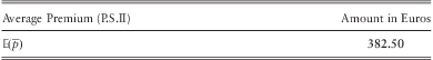
The results of Table 10 (see also Figure 3) are also similar with those of the Premium Strategy I, since the five insurance companies have premiums significantly below the market average premium of 382.50€ for a break-even premium rate of 20–40%.

Table 10 (The optimal premium strategy in Euro for the 5 Greek insurance companies that have $$\[--><$>{\Bbb E}\left( {{{\theta }_k}} \right)\, \gt \,10,000<$><!--\]$$ for the different values of the break-even premium rate).

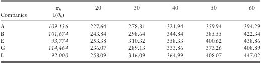
Figure 3 Optimal premium for the year 2010 (Premium Strategy II).

Now, if we would like to compare the findings of the two Premium Strategies, we can easily see that the Premium Strategy II is cheaper (i.e. it provides lower premiums) than the Premium Strategy I for all the A, B, E, G and L insurance companies. This result was expected, as in the Greek insurance market, the leader (dominator) companies have expensive premiums, above the average premium of the market.