


1. Introduction
Consider the following planar system
 \begin{equation} \dot x ={-} y + P(x, y), \;\; \dot y = x+ Q(x, y), \end{equation}
where  $P,Q$ are real analytic functions in
  $x, y$ without constant and linear terms, which implies that the origin is an equilibrium point.
The centre-focus (or centre) problem, originally defined for (1.1) in the polynomial setting, consists of obtaining conditions on the coefficients of the system to distinguish when the origin is either a focus or a centre. It is one of the main and oldest problems in side of the qualitative theory of ordinary differential equations and has been the subject of intensive research (see [Reference Christopher6, Reference Romanovski and Shafer36] and references therein). We recall that an equilibrium point  $p$ is a centre if all orbits sufficiently closed to it are periodic, and
  $p$ is a focus if there is a neighbourhood
  $V$ of
  $p$ such that all the orbits by points of
  $V\setminus \{p\}$ spiral either in forward or in backward time to
  $p$.
$p$.
The study of the period function and isochronicity is another important area of research related to system (1.1). We say that the origin of system (1.1) is isochronous centre if it is a centre and the period function, i.e. the function that associates to each periodic orbit its minimal period, defined in a small enough neighbourhood of the origin is constant. The study of isochronicity probably started before the development of the differential calculus. In the XVI century, Galileo Galilei considered this problem when studying the classical pendulum. After, in XVII century, Huygens studied the cycloidal pendulum [Reference Fowles15]. This pendulum has isochronous oscillations in opposition to the classical one. Huygens applied his results to the construction of clocks. However, only in the second half of the last century the isochronicity of centres of planar polynomial vector fields have been extensively studied, see [Reference Chavarriga and Sabatini5, Reference Freire, Gasull and Guillamon16, Reference Han and Romanovski27].
A particularly important class of isochronous centres are those which rotate around the origin with the constant angular speed (see e.g. [Reference Conti10, Reference Dias and Mello12, Reference Llibre and Rabanal28]). Centres with this property are referred to as rigid centres. In this case the centre-focus problem is equivalent to the isochronicity problem and this is one of the reasons why several authors have been interested for this type of centres. Probably, the easiest way to formally define the rigid centres is by making reference to polar coordinates. We say that system (1.1) is a rigid system, if in polar coordinates  $(x, y)\mapsto (r \cos \theta , r \sin \theta )$ it takes the form
 \begin{equation} \begin{aligned} & \dot r = \cos\theta P(r \cos\theta, r \sin\theta)+\sin\theta Q(r \cos\theta, r \sin\theta),\\ & \dot \theta =1. \end{aligned} \end{equation}
The emphasis in expression (1.2) is only on the angular speed, which in the rigid systems is constant. Note that unitary angular speed ( $\dot \theta = 1$) is a consequence of the normalized framework (1.1). Moreover, system (1.2) is equivalent to a generalized Abel differential equation, see [Reference Cima, Gasull and Mañosas7]. This is another reason to study this type of systems. If the origin is a centre of system (1.1), and it is rigid, then we say that the origin is a rigid centre. In [Reference Algaba and Reyes1] the authors find conditions for a rigid system to have an analytical commutator, and so they are able to solve the centre problem for several families of rigid systems. Collins, in [Reference Collins8], obtained explicit algebraic formulas that solve the centre problem for a particular class of rigid systems. Collins also solved the centre problem for polynomial cubic rigid systems, see [Reference Collins9]. The existence and uniqueness of limit cycles of rigid systems also are subjects of great interest, see e.g. [Reference Gasull, Prohens and Torregrosa21, Reference Gasull and Torregrosa22].
In this paper, we deal with tridimensional systems having a centre on the center manifold at the origin. Therefore, consider the following tridimensional system
 \begin{equation} \dot x ={-} y + P(x, y, z), \;\; \dot y = x+ Q(x, y, z),\;\; \dot z ={-}\lambda z + R(x, y, z), \end{equation}
where  $\lambda \neq 0$ and
  $P$,
$P$,  $Q$,
$Q$,  $R$ are analytic in
  $x$,
$x$,  $y$ and
  $z$ without constant and linear terms, which implies that the origin is an equilibrium point. Following the centre manifold theorem, for every
  $k\in {\mathbb {N}}$, there exists a local two-dimensional
  $\mathcal {C}^{k}$ invariant manifold
  $\mathcal {W}^{c}$ tangent to
  $z=0$ at the origin. In general, the invariant manifold
  $\mathcal {W}^{c}$ is neither unique nor analytic.
The concept of centre for system (1.3) extends naturally due to the existence of centre manifold in the vicinity of the origin. This problem has been the subject of several recent papers. In [Reference Edneral, Mahdi, Romanovski and Shafer14] the authors describe an algorithm to solve the centre problem for system (1.3) on the center manifold and they prove that to fixed value of  $\lambda$ the set of systems of form (1.3), with
  $P$,
$P$,  $Q$ and
  $R$ polynomials, having a centre on the local center manifold at the origin corresponds to a variety in the space of admissible coefficients. The authors of [Reference Buică, García and Maza4] prove that the origin of system (1.3) is a centre on the center manifold if and only if there exists a local analytic inverse Jacobi multiplier. Using Lie algebra techniques, in [Reference García, Maza and Shafer18], the authors obtain a criterion for the origin to be a focus or a centre for systems of the form (1.3), and for it to be linearizable. In [Reference García, Maza and Shafer19] the authors prove that it is possible to bound the cyclicity of centres at the origin of system (1.3) and in [Reference García, Maza and Shafer20] the same authors provide upper bounds on the cyclicity of centres on center manifolds in the well-known Lorenz family, and also in the Chen and Lü families. The centre problem on the center manifold for Lü family is solved in [Reference Mahdi, Pessoa and Shafer31] and for the Moon-Rand family is studied in [Reference Giné and Valls24, Reference Mahdi, Romanovski and Shafer32]. Partial results about the centre problem on center manifolds for quadratic families, i.e. for systems of the form (1.3) with
  $P$,
$P$,  $Q$ and
  $R$ quadratic polynomials, were obtained in [Reference Giné and Valls23]. Mahdi in [Reference Mahdi29] partially solves the centre problem on center manifolds for quadratic systems of the form (1.3) obtained from a third-order differential equation. In [Reference Mahdi, Pessoa and Hauenstein30] the authors complete this study and, for the first time in the literature, they propose a new hybrid symbolic-numerical approach to solve the centre problem.
We focus on studying the rigid systems in  $ {\mathbb {R}}^{3}$. More precisely, we studying the centre-focus problem to the systems of the form
 \begin{equation} \dot x ={-} y + x F(x, y, z), \;\; \dot y = x+ yF(x, y, z),\;\; \dot z ={-} \lambda z + R(x, y, z). \end{equation}
This system restricted to a center manifold is rigid. Moreover, in cylindrical coordinates, their orbits rotate around the  $z$-axis with the constant angular speed. In fact, if system (1.3), in cylindrical coordinates, has constant angular speed, then it has the form above (see proposition 2.4). However, there are systems of the form (1.3) which, when restricted to a center manifold, are rigid, but cannot be written in the form (1.4) (see proposition 2.6).
Motivated by the results of Conti [Reference Conti10] on the characterization of the rigid centres for homogeneous rigid systems on the plane, we divided the study of the systems of the form (1.4) in two class, homogeneous rigid systems and non-homogeneous rigid systems. The paper is structured as follows.
In § 2 we introduce the rigorous definitions of rigid systems in  $\mathbb {R}^{3}$ and rigid systems in
  $\mathbb {R}^{3}$ by cylindrical coordinates and we characterized these types of systems through normal forms (see propositions 2.3, 2.4 and corollary 2.5). We also showed that these definitions are not equivalents (see proposition 2.6).
In § 3 we study the homogeneous rigid systems, i.e. systems of the form (1.4) with  $F=F_n$ and
  $R=R_m$, where
  $F_n$ and
  $R_m$ are homogenous polynomials of degree
  $n$ and
  $m$, respectively. We prove that se
  $R_m(x, y, 0)\equiv 0$ or
  ${\partial F_n}/{\partial z}\equiv 0$, then the origin of system (1.4) is a centre if and only if
  $\int _0^{2\pi } F_n(\cos \theta , \sin \theta , 0)\textrm {d}\theta =0$ (see propositions 3.1 and 3.2).
Assuming the hypothesis  ${\partial R_m}/{\partial z}\equiv 0$, in § 4, we classify the centres of systems of the form (1.4) with
  $F=F_n$ and
  $R=R_m$, where
  $F_n$ and
  $R_m$ are homogenous polynomials of degree
  $n$ and
  $m$, for the follows cases:
•
 $n=1$ and $m=2$;
•
$n=1$, $m=3, 4$ and $\lambda =1$;•
$n=2$, $m=2, 3$ and $\lambda =1$.


In the case  $n=2$,
  $m=3$ and
  $\lambda =1$, we have used modular arithmetic to do the study and so we are not sure if the classification is complete, but we conjecture that yes. Excluding the hypothesis
  ${\partial R_m}/{\partial z}\equiv 0$, we obtain several families of centres for the case
  $n=1$,
  $m=2$ and
  $\lambda =1$. These families were also obtained using modular arithmetic and, as in the previous case, we are not sure if are all the families of centres, although we believe so. We complete § 4 classifying the centres of the case
  $n=m=2$,
  $\lambda =1$ and
  $F_2=R_2$.
In § 5 we consider non-homogeneous rigid systems. More precisely, we study some systems of the form (1.4) where  $F$ is a polynomial in a unique variable, i.e. the variable
  $z$, and
  $R$ is a homogenous polynomial in three or two variables. This study was motivated by interesting results obtained in [Reference Dias and Mello12, Reference Llibre and Rabanal28] for the equivalent cases in the plane.
2. Rigid systems in $ {\mathbb {R}}^{3}$

Similarly as in the  $ {\mathbb {R}}^{2}$, the most natural way to define rigidity is by expressing the system restricted to a center manifold in polar coordinates.
Definition 2.1 (rigid systems in  $ {\mathbb {R}}^{3}$)
We say that the tridimensional system (1.3) is rigid if its restriction to a center manifold by the origin, in the polar coordinates, has the form (1.2). Moreover, if the origin is a centre on the center manifold, then we say that the origin is a rigid centre.
The above definition is not very practical for computations, since to study rigid centres in  $\mathbb {R}^{3}$ we have the additional difficulty of restricting system (1.3) to a center manifold. For to avoid this task, we will introduce a subclass of rigid systems.
Definition 2.2 (rigid systems in  $ {\mathbb {R}}^{3}$ by cylindrical coordinates)
We say that the tridimensional system (1.3) is rigid by cylindrical coordinates if, in cylindrical coordinates  $(x, y, z)\mapsto (r \cos \theta , r \sin \theta , z)$, it assumes the following form
 \begin{equation} \begin{aligned} & \dot r =\cos\theta P(r \cos\theta, r \sin\theta, z)+\sin\theta Q(r \cos\theta, r \sin\theta, z),\\ & \dot\theta = 1,\\ & \dot z ={-}\lambda z + R(r \cos\theta, r \sin\theta, z). \end{aligned} \end{equation}
 The right-hand expressions of the first and third equations in (2.1) are irrelevant to the definition. The emphasis is in the second equation of (2.1), it shows that the orbits of the system rotates around the  $z$-axis with the constant angular speed.
We will see that the above definitions are not equivalent (see proposition 2.6). In fact the rigid systems in  $ {\mathbb {R}}^{3}$ by cylindrical coordinates are a subclass of rigid systems in
  $ {\mathbb {R}}^{3}$.
The following propositions characterize systems (1.3) that are rigid and rigid by cylindrical coordinates.
Proposition 2.3 System (1.3) is rigid if and only if its restriction to a center manifold by the origin takes the following canonical form
 \begin{equation} \dot x ={-} y + x F(x, y), \;\; \dot y = x+ yF(x, y), \end{equation}
where  $F$ is a
  $\mathcal {C}^{k}$ map, defined in a small enough neighbourhood of origin, for any
  $1\leq k<\infty$.
Proof. In polar coordinates  $(x, y)\mapsto (r \cos \theta , r \sin \theta )$, system (2.2) can be written as
 \[ \dot r = r F(r \cos \theta, r \sin \theta), \;\; \dot \theta = 1. \]
Thus by definition the system is a rigid system.
Now we show the converse. By the centre manifold theorem, for every  $k\in {\mathbb {N}}$, there exists a two-dimensional
  $\mathcal {C}^{k}$ invariant manifold
  $\mathcal {W}^{c}$ tangent to
  $z=0$ at the origin and so
  $\mathcal {W}^{c}$ is locally the graphic of a
  $\mathcal {C}^{k}$ map
  $z=h(x, y)$ (see theorem 3.2.1 in p. 127 of [Reference Guckenheimer and Holmes26]). Hence, system (1.3) restricted to
  $\mathcal {W}^{c}$ takes the form
 \begin{equation} \dot x ={-} y + \tilde{P}(x, y), \;\; \dot y = x+ \tilde{Q}(x, y), \end{equation}
where  $\tilde {P}(x, y)=P(x, y,h(x, y))$ and
  $\tilde {Q}(x, y)=Q(x, y,h(x, y))$. In polar coordinates system (2.3) becomes
 \begin{equation} \begin{aligned} & \dot r = \cos \theta \; \tilde{P}(r \cos \theta, r \sin \theta) +\sin \theta \;\tilde{Q}(r \cos \theta, r \sin \theta),\\ & \dot \theta = 1+\frac{1}{r}\big[\cos \theta \; \tilde{Q}(r \cos \theta, r \sin \theta) -\sin \theta \;\tilde{P}(r \cos \theta, r \sin \theta)\big]. \end{aligned} \end{equation}
By the rigidity assumption applied to system (1.3) (i.e.  $\dot \theta = 1$), we immediately obtain of (2.4) that
 \begin{equation} \frac{1}{r}\big[\cos \theta \; \tilde{Q}(r \cos \theta, r \sin \theta) -\sin \theta \;\tilde{P}(r \cos \theta, r \sin \theta)\big]=0. \end{equation}
In the  $(x, y)$ coordinates equation (2.5) is written as
 \begin{equation} x \tilde{Q}(x, y)-y \tilde{P}(x, y) = 0. \end{equation}
Equation (2.6) implies that  $y\tilde {P}(0,y)=0$, that is
  $\tilde {P}(0,y)=0$. Using Hadamard's lemma (see [Reference Bierstone3]), there exists a
  $\mathcal {C}^{k}$ map
  $F(x, y)$ such that
  $\tilde {P}(x, y)=xF(x, y)$. Similarly, we obtain
  $\tilde {Q}(x, y)=yG(x, y)$, where
  $G$ is a
  $\mathcal {C}^{k}$ map. Thus, from (2.6), we readily obtain
  $xy(G(x, y)-F(x, y))=0$, i.e.
  $G(x, y)=F(x, y)$. Therefore,
  $\tilde {P}(x, y)=xF(x, y)$ and
  $\tilde {Q}(x, y)=yF(x, y)$, which proves the proposition.
Proposition 2.4 System (1.3) is rigid by cylindrical coordinates if and only if it takes the following canonical form
 \begin{equation} \dot x ={-} y + x F(x, y, z), \;\; \dot y = x+ yF(x, y, z),\;\; \dot z ={-} \lambda z + R(x, y, z), \end{equation}
where  $F$ is an analytic map.
Proof. In cylindrical coordinates  $(x, y, z)\mapsto (r \cos \theta , r \sin \theta , z)$, system (2.7) can be written as
 \[ \dot r = r F(r \cos \theta, r \sin \theta, z), \;\; \dot \theta = 1,\;\; \dot z ={-}\lambda z + R(r \cos \theta, r \sin \theta, z), \]
thus by definition the system is a rigid system.
Now we show the converse. In cylindrical coordinates system (1.3) takes the form
 \begin{equation} \begin{aligned} & \dot r = \cos \theta \; P(r \cos \theta, r \sin \theta, z) +\sin \theta \;Q(r \cos \theta, r \sin \theta, z),\\ & \dot \theta = 1+\frac{1}{r}\big[\cos \theta \; Q(r \cos \theta, r \sin \theta, z) +\sin \theta \;P(r \cos \theta, r \sin \theta, z)\big],\\ & \dot z ={-}\lambda z + R(r \cos \theta, r \sin \theta, z). \end{aligned} \end{equation}
By the rigidity assumption applied to system (1.3) (i.e.  $\dot \theta = 1$), we immediately obtain of (2.8) that
 \begin{equation} \frac{1}{r}\big[\cos \theta \; Q(r \cos \theta, r \sin \theta, z) +\sin \theta \;P(r \cos \theta, r \sin \theta, z)\big]=0. \end{equation}
In the  $(x, y, z)$ coordinates equation (2.9) is written as
 \begin{equation} x Q(x, y, z)-y P(x, y, z) = 0. \end{equation}
Equation (2.10) implies that  $yP(0,y, z)=0$, i.e.
  $P(0,y, z)=0$. Therefore, there exists an analytic map
  $F$ such that
  $P(x, y, z)=xF(x, y, z)$. Similarly, we obtain
  $Q(x, y, z)=yG(x, y, z)$, where
  $G$ is analytic. Thus, from (2.10), we readily obtain
  $x y (G(x, y, z)-F(x, y, z))=0$, i.e.
  $G(x, y, z)=F(x, y, z)$. Therefore,
  $P(x, y, z)=xF(x, y, z)$ and
  $Q(x, y, z)=yF(x, y, z)$, which proves the proposition.
The following corollary is a straightforward consequence of the proofs of the above propositions.
Corollary 2.5 Consider system (1.3). Then
(a) this system is rigid if and only if
$xQ(x, y, z)-yP(x, y, z)\equiv 0$ with $z=h(x, y)$, where $h$ is the local expression of an invariant center manifold $\mathcal {W}^{c}$;(b) this system is rigid by cylindrical coordinates if and only if
$xQ(x, y, z)-yP(x, y, z)\equiv 0$.


It is obvious that if system (1.3) is rigid by cylindrical coordinates, then it is rigid in  $\mathbb {R}^{3}$. However, the next proposition shows that definitions 2.1 and 2.2 are not equivalent. In fact the rigid systems in
  $ {\mathbb {R}}^{3}$ by cylindrical coordinates are a subclass of rigid systems in
  $ {\mathbb {R}}^{3}$.
Proposition 2.6 The system
 \begin{align} \dot x &={-} y +x^{2}+xy+xz+yz+z^{2}, \quad \dot y = x+xy+xz+y^{2}+yz+z^{2},\notag\\ \dot z &={-}z + xz+yz+z^{2}, \end{align}
is rigid, but is not rigid by cylindrical coordinates. Moreover, the origin is a centre of it on the center manifold.
Proof. Note that  $z$ is a common factor on the right side of the last equation of system (2.11). Therefore, the plane
  $z=0$ is invariant by the flow generated by system (2.11) and so it is a center manifold of this system. System (2.11) restricted to plane
  $z=0$ is given by
 \[ \dot x ={-} y + x^{2}+xy, \;\; \dot y = x+ xy+y^{2}. \]
This system is rigid and has the following first integral
 \[ H(x, y)=\dfrac{x^{2}+y^{2}}{(1-x+y)^{2}}, \]
which it is defined in the origin. Thus, system (2.11) is rigid and has a centre on the center manifold.
Now, system (2.11) is not rigid by cylindrical coordinates, because
 \[ xQ(x, y, z)-yP(x, y, z)=x^{2}z+xz^{2}-y^{2}z-yz^{2}\not\equiv 0, \]
where  $P(x, y, z)=x^{2}+xy+xz+yz+z^{2}$ and
  $Q(x, y, z)=xy+xz+y^{2}+yz+z^{2}$.
Remark 2.7 For some cases, the centre-focus problem in center manifolds of rigid system in  $\mathbb {R}^{3}$ by cylindrical coordinates is exactly the same problem to rigid system in
  $\mathbb {R}^{2}$. For instance, when
  $R$ in (2.7) satisfies
  $R(x, y, 0)\equiv 0$, i.e. when we can write
  $R(x, y, z)=z\tilde {R}(x, y, z)$ with
  $\tilde {R}\in \mathbb {R}[x, y, z]$. In this case
  $z=0$ is a center manifold and system (2.7) restricted to it becomes
 \[ \dot x ={-} y + x F(x, y,0), \;\; \dot y = x+ yF(x, y,0), \]
where  $F(x, y,0)\in {\mathbb {R}}[x, y]$ is a polynomial without a constant term. Thus, the results about rigid systems in
  $\mathbb {R}^{2}$ are naturally extended to this class of rigid system in
  $\mathbb {R}^{3}$.
Another class of rigid systems in  $\mathbb {R}^{3}$ by cylindrical coordinates which the results about centre-focus problems are naturally extensions of the results in the plane are systems of form (2.7) with
  $({\partial F}/{\partial z})(x, y, z)\equiv 0$, i.e. when we can write
  $F(x, y, z)=F(x, y)$ with
  $F\in \mathbb {R}[x, y]$. In this case the two first equations in system (2.7) are uncoupled with the last one and so, system (2.7) restricted to any center manifold is given by
 \[ \dot x ={-} y + x F(x, y), \;\; \dot y = x+ yF(x, y). \]
3. Homogeneous rigid systems in $ {\mathbb {R}}^{3}$

Consider the following system
 \begin{equation} \dot x ={-} y + x F_n(x, y, z), \;\; \dot y = x+ yF_n(x, y, z),\;\; \dot z ={-} \lambda z + R_m(x, y, z), \end{equation}
where  $F_n, R_m\in {\mathbb {R}}[x, y, z]$ are homogenous polynomial in
  $x, y, z$ of degree
  $n\geq 1$, and
  $m\geq 2$, respectively. System (3.1) are called homogeneous rigid systems. In this section we will prove some propositions about these systems.
The next two prepositions are motivated by well-known results that characterize the centres of planar homogenous rigid system, see e.g. [Reference Conti10, Reference Conti11].
Proposition 3.1 Consider system (3.1) with  $R_m(x, y,0)\equiv 0$. Then system (3.1) has a rigid centre at the origin if and only if
 \[ \int^{2\pi} _0F_n(\cos (s), \sin(s),0)\textrm{d}s=0. \]
Proof. By remark 2.7 the plane  $z=0$ is the center manifold by the origin of system (3.1). Hence, restricted to plane
  $z=0$, system (3.1) in polar coordinates
  $x = \rho \cos \theta$,
  $y = \rho \sin \theta$ becomes
 \[ \dot \rho = \rho^{n+1} F_n(\cos \theta, \sin \theta, 0), \;\; \dot \theta = 1. \]
The above system is equivalent to the differential equation
 \[ \dfrac{\textrm{d}\rho}{\textrm{d}\theta}=F_n(\cos \theta, \sin \theta,0) \rho^{n+1}. \]
As  $F_n$ is not constant, separating the variables
  $\rho$ and
  $\theta$ of this equation, and integrating between
  $0$ and
  $\theta$ we get that its solution satisfies
 \[ \rho(\theta)^{n} =\dfrac{\rho (0)^{n}}{1-n\rho (0)^{n}\int^{\theta}_0 F_n(\cos (s), \sin(s),0)\textrm{d}s}. \]
Hence, the origin is a centre in a center manifold to system (3.1) with  $n\geq 1$ and
  $R_m(x, y,0)\equiv 0$, if and only if
 \[ \int^{2\pi} _0F_n(\cos (s), \sin(s),0)\textrm{d}s=0. \]
Observe that, if  $n$ is odd, the above integral is always zero. This completes the proof of the proposition.
Proposition 3.2 Consider system (3.1) with  $({\partial F_n}/{\partial z})(x, y, z)\equiv 0$, i.e.
  $F_n(x, y, z)=F_n(x, y)$ is a homogeneous polynomial in the variables
  $x$,
$x$,  $y$. Then system (3.1) has a rigid centre at the origin if and only if
 \[ \int^{2\pi} _0F_n(\cos (s), \sin(s))\textrm{d}s=0. \]
Proof. By remark 2.7, system (3.1) restricted to a center manifold at origin is given by
 \begin{equation} \dot x ={-} y + x F_n(x, y), \;\; \dot y = x+ yF_n(x, y). \end{equation}
Hence, in polar coordinates  $x = \rho \cos \theta$,
  $y = \rho \sin \theta$, system (3.2) becomes
 \[ \dot \rho = \rho^{n+1} \; F_n(\cos \theta, \sin \theta), \;\; \dot \theta = 1, \]
which is equivalent to the differential equation
 \[ \dfrac{\textrm{d}\rho}{\textrm{d}\theta}=F_n(\cos \theta, \sin \theta) \rho^{n+1}. \]
As in the proof of previous proposition, the solution of this equation with initial condition  $\rho (0)=\rho _0$ is
 \begin{equation} \begin{aligned} \rho(\theta) & =\dfrac{\rho_0}{\left(1-n\rho_0^{n}\int^{\theta}_0 F_n(\cos ({s}), \sin({s}))\textrm{d}s\right)^{{1}/{n}}}. \end{aligned} \end{equation}
Now, system (3.1) have a periodic orbit by the point  $(\rho _0, 0, z_0)$ if and only if
  $\rho (2\pi )=\rho _0$. Hence, by equation (3.3), we have that
 \[ \int^{2\pi} _0F_n(\cos ({s}), \sin({s}))\textrm{d}s =0. \]
Here  $z_0=h(\rho _0, 0)$, where
  $z=h(x, y)$ is a local expression of center manifold. Observe that, if
  $n$ is odd, the above integral is always zero. This completes the proof of the proposition.
In the study of centre-focus problem for homogeneous rigid systems in  $\mathbb {R}^{3}$, the above propositions given us two centre conditions. The first centre conditions are the value parameters from system (3.1) such that
  $R_m(x, y,0)\equiv 0$ and
  $\int ^{2\pi } _0F_n(\cos (\theta ), \sin (\theta ),0)\textrm {d}\theta =0$. The second centre conditions are the value parameters from system (3.1) such that
  $({\partial F_n}/{\partial z})(x, y, z)\equiv 0$ and
  $\int ^{2\pi } _0F_n(\cos (\theta ), \sin (\theta ))\textrm {d}\theta =0$. We call this conditions of elementary centre conditions for homogeneous rigid systems (or simply elementary centre conditions when there is no confusion with others types of rigid systems).
4. Centre problem for some classes of homogeneous rigid systems in $ {\mathbb {R}}^{3}$

In this section we study the centres at the origin on the center manifold of some class of homogeneous rigid systems in  $ {\mathbb {R}}^{3}$. For do this, we summarize the method described in [Reference Edneral, Mahdi, Romanovski and Shafer14] (see also [Reference Mahdi29, Reference Mahdi, Pessoa and Hauenstein30, Reference Mahdi, Romanovski and Shafer32]) for studying the centre problem on a center manifold for vector fields in
  $\mathbb {R}^{3}$.
Consider system (1.3), the Lyapunov centre theorem states that this system has a centre at the origin on the center manifold if and only if the system has an analytic first integral defined in the origin of the form  $H(x, y, z) = x^{2} +y^{2} +\cdots$, where the dots mean higher order terms (see [Reference Bibikov2, Reference Edneral, Mahdi, Romanovski and Shafer14]). In what follows we consider that
  $P$,
$P$,  $Q$ and
  $R$ in (1.3) are polynomials. We start by introducing the complex variable
  $u = x + iy$. Therefore, the first two equations in (1.3) are equivalent to the unique equation
  $\dot {u} = iu + \cdots$. Adding to this equation its complex conjugate, changing
  $\bar {u}$ (where as usual
  $\bar {u}$ denote the conjugate of
  $u$) by
  $v$, thinking in
  $v$ as an independent complex variable, and substituting
  $z$ by
  $w$, we obtain the following complexification of system (1.3):
 \begin{equation} \begin{aligned} \dot{u} & = iu+\displaystyle\sum^{n}_{p+q+r=2}a_{pqr} u^{p} v^{q} w^{r}, \\ \dot{v} & = -iv+\displaystyle\sum^{n}_{p+q+r=2}b_{pqr} u^{p} v^{q} w^{r}, \\ \dot{w} & = \beta w+\displaystyle\sum^{n}_{p+q+r=2}c_{pqr} u^{p} v^{q} w^{r}, \end{aligned} \end{equation}
where  $b_{qpr} = \bar {a}_{pqr}$ and the
  $c_{pqr}$ are such that
  $\sum ^{n}_{p+q+r=2} c_{pqr} u^{p} \bar {u}^{q} w^{r}$ is real for all
  $u\in \mathbb {C}$ and
  $w\in \mathbb {R}$. Denote by
  $X$ the new vector field associated with system (4.1) on
  $\mathbb {C}^{3}$. Now the existence of a first integral
  $H(x, y, z) = x^{2} + y^{2} + \cdots$ for a system (1.3) is equivalent to the existence of a first integral of the form
 \[ H(u,v,w)=uv+\sum_{j+k+l=3} v_{jkl} u^{j} v^{k} w^{l} \]
for system (4.1).
By computing the coefficients of  $XH=\langle X, \nabla H\rangle$ and equating them to zero, we investigate the existence of a first integral
  $H$ for a system (4.1). Denoting by
  $g_{k_1k_2k_3}$ the coefficient of
  $u^{k1} v^{k2} w^{k3}$ in
  $XH$, except when
  $(k_1,k_2,k_3) = (k, k, 0)$ for a positive integer
  $k$, we can solve in a unique way for
  $v_{k_1k_2k_3}$ the equation
  $g_{k_1k_2k_3}$ = 0 in terms of the known quantities
  $v_{\alpha \beta \gamma }$ such that
  $\alpha +\beta +\lambda < k_1+k_2+k_3$. Hence, if
  $g_{kk0} = 0$ for all
  $k\in \mathbb {N}$ a formal first integral
  $H$ exists. When the coefficient
  $g_{kk0}$ is non-zero an obstruction to the existence of the formal series
  $H$ occurs. Such coefficient is called the
  $k$th focus quantity.
The focus quantities  $g_{110} = 0$ and
  $g_{220}$ are determined in a unique way, but the others depend on the choices made for
  $v_{kk0}$,
  $k \in \mathbb {N}$,
  $k\geq 2$. Once such computations are made,
  $H$ is determined and satisfies
 \[ XH(u,v,w) = g_{220} (uv)^{2} + g_{330} (uv)^{3} +\cdots . \]
It follows that if for one choice of the  $v_{kk0}$ at least one focus quantity is non-zero, the same is true for every other choice of the
  $v_{kk0}$. A sufficient and necessary condition for the existence of a centre on the center manifold is to vanish all focus quantities, otherwise we have a focus (see [Reference Edneral, Mahdi, Romanovski and Shafer14]).
Theorem 4.1 Consider system (3.1) with  $({\partial R_m}/{\partial z})(x, y, z)\equiv 0$, i.e. system
 \begin{equation} \dot x ={-} y + x F_n(x, y, z), \;\; \dot y = x+ yF_n(x, y, z), \; \; \dot z ={-} \lambda z + R_m(x, y), \end{equation}
where  $F_n(x, y, z)=\sum _{j+k+l=n} a_{jkl} x^{j} y^{k} z^{l}$ and
 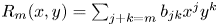 $R_m(x, y)=\sum _{j+k=m} b_{jk} x^{j} y^{k}$.
(a) If
$n=1$ and $m=2$, system (4.2) has a centre at the origin on the center manifold if and only if $a_{001}=0$ or $b_{20}=b_{11}=b_{02}=0$.(b) If
$\lambda =n=1$ and $m=3, 4$, system (4.2) has a centre at the origin on the center manifold if and only if $a_{001}=0$ or $b_{jk}=0$ for all $j$, $k\in \mathbb {N}$ with ${j+k=3, 4}$.(c) If
$\lambda =1$, $n=2$, and $m=2$, system (4.2) has a centre at the origin on the center manifold if and only if $a_{200}=-a_{020}$ and $a_{101}=a_{011}=a_{002}=0$ or $a_{200}=-a_{020}$ and $b_{20}=b_{11}=b_{02}=0$.(d) If
$\lambda =1$, $n=2$, $m=3$, and $a_{200}=-a_{020}$, $a_{101}=a_{011}=a_{002}=0$ or $a_{200}=-a_{020}$, $b_{30}=b_{21}=b_{12}=b_{03}=0$, then system (4.2) has a centre at the origin on the center manifold.


Proof. First we prove statement (a). Using the method described above, we have that the first focus quantity associated with origin of system (4.2) is
 \[ g_{220}=\frac{a_{001}(b_{20} + b_{02})}{\lambda}. \]
Therefore,  $a_{001}=0$ or
  $b_{02}=-b_{20}$ are necessary conditions to have a centre at the origin on the center manifold of system (4.2). Note that
  $a_{001}=0$ is also sufficient, because it is an elementary centre condition by proposition 3.2.
Now, assume that  $a_{001}\neq 0$ and
  $b_{02}=-b_{20}$. First we suppose that
  $a_{100}=a_{010}=0$. In this case
  $g_{220}=0$ and the second focus quantity is
 \[ g_{330}={-}\frac{a_{001}^{2} \left(4 b_{20}^{2}+b_{11}^{2}\right)}{2 \lambda \left(\lambda ^{2}+4\right)}. \]
So  $b_{20}=b_{11}=b_{02}=0$ is a necessary condition to have a centre at the origin on the center manifold of system (4.2). It is also a sufficient condition, because it is an elementary centre condition by proposition 3.1.
If  $a_{100}^{2}+a_{010}^{2}\neq 0$, we can assume that system (4.2) is given by
 \begin{equation} \dot x ={-} y + x(y+z), \;\; \dot y = x+ y(y+z),\;\; \dot z ={-} \lambda z + b_{20}x^{2}+b_{11}xy-b_{20}y^{2}. \end{equation}
Otherwise, we do the change of variables
 \begin{align} x &= \frac{a_{010}}{a_{100}^{2}+a_{010}^{2}}X+ \frac{a_{100}}{a_{100}^{2}+a_{010}^{2}}Y,\notag\\ y &={-}\frac{a_{100}}{a_{100}^{2}+a_{010}^{2}}X+ \frac{a_{010}}{a_{100}^{2}+a_{010}^{2}}Y,\;\; z = \frac{1}{a_{001}}Z. \end{align}
The first focus quantity  $g_{220}$ of system (4.3) is zero and the next four
  $g_{kk0}$,
  $k=3, 4, 5, 6$, can be easily computed (their expressions are too lengthy and we omit them here), for instance using software of symbolic computations like Maple [33] or Mathematica [37] (see the appendix from [Reference Mahdi, Romanovski and Shafer32] for a Mathematica code for computing the focus quantities). We have that the focus quantities
  $g_{kk0}$,
  $k=3, 4, 5, 6$ are rational expressions and the Groebner basis of the ideal generated by its numerators is given by the polynomials:
 \begin{align*} & \{ b_{11}^{2} \left(4 b_{20}^{2}+b_{11}^{2}\right), \;b_{20} b_{11} \left(4 b_{20}^{2}+b_{11}^{2}\right), \; (2 b_{20}-b_{11}) (2 b_{20}+b_{11}) \left(4 b_{20}^{2}+b_{11}^{2}\right),\\ & \quad -\left(4 b_{20}^{2}+b_{11}^{2}\right) (23 b_{20}-3 b_{11} \lambda), \; b_{20} \left(\lambda^{2}+4\right) \left(4 b_{20}^{2}+b_{11}^{2}\right),\\ & \quad -308 b_{20}^{3}+116 b_{20}^{2} \lambda^{2}+476 b_{20}^{2}-77 b_{20} b_{11}^{2}-24 b_{20} \lambda^{2}-96 b_{20}\\ & \quad+29b_{11}^{2} \lambda^{2}+119 b_{11}^{2}+4 b_{11} \lambda^{3}+16 b_{11} \lambda,\\ & \quad -1024 b_{20}^{3} \lambda-492 b_{20}^{2} b_{11}+24 b_{20}^{2} \lambda^{3}+96 b_{20}^{2} \lambda-256 b_{20} b_{11}^{2} \lambda+36 b_{20} b_{11} \lambda^{2}\\ & \quad +144 b_{20} b_{11}-123 b_{11}^{3},308 b_{20}^{3}-132 b_{20}^{2} \lambda^{2}-492 b_{20}^{2}+77 b_{20} b_{11}^{2}+4 b_{20} \lambda^{4}+52 b_{20} \lambda^{2}\\ & \quad +144 b_{20}-33 b_{11}^{2} \lambda^{2}-123 b_{11}^{2}\}. \end{align*}
The above polynomials are all null if and only if  $b_{20}=b_{11}=0$. By proposition 3.1, this is an elementary centre condition for system (4.3) and so it has a centre at the origin on the center manifold if and only if
  $b_{20}=b_{11}=0$. This complete the proof of statement (a).
To prove statement (b), as in statement (a), we also distinguish the three cases  $\{a_{001}=0\}$,
  $\{a_{001}\neq 0, a_{100}=a_{010}=0\}$ and
  $\{(a_{100}^{2}+a_{010}^{2})a_{001}\neq 0\}$. By proposition 3.2,
  $a_{001}=0$ is an elementary centre condition for system (4.2) (with
  $\lambda =n=1$) and so it has a centre at the origin on the center manifold. When
  $a_{100}=a_{010}=0$ and
  $a_{001}\neq 0$, we have that for
  $n=1$ and
  $m=3$ the three first focal quantities are
  $g_{220}=g_{330}=0$ and
 \[ \begin{aligned} g_{440} & ={-}\frac{3}{160} a_{001}^{2} \left(\frac{56 b_{30}^{2}}{5}+(b_{30}+b_{12})^{2}+\left(\frac{13 b_{30}}{\sqrt{5}}+\sqrt{5} b_{12}\right)^{2}+(b_{21}+b_{03})^{2}\right.\\ & \:\:\:\:\: \left.+ \left(\sqrt{5} b_{21}+\frac{13 b_{03}}{\sqrt{5}}\right)^{2}+\frac{56 b_{03}^{2}}{5}\right). \end{aligned} \]
In this case system (4.2) has a centre at the origin on the center manifold if and only if  $b_{30}=b_{21}=b_{12}=b_{03}=0$, because it is an elementary centre condition by proposition 3.1. Now, for
  $n=1$ and
  $m=4$ the two first focal quantities are
  $g_{220}=0$ and
 \[ g_{330}=\frac{1}{4} a_{001} (3 b_{40}+b_{22}+3 b_{04}). \]
Hence,  $b_{22}=-3( b_{40}+b_{04})$ is a necessary condition to have a centre at the origin on the center manifold of system (4.2) in this case. Assuming this last condition, it follows that the next two focal quantities are
  $g_{440}=0$ and
 \[ g_{550}={-}\frac{a_{001}^{2}}{1360} (64 b_{40}^{2}+32 (3 b_{40}-2 b_{04})^{2}+10 b_{31}^{2}+63 (b_{31}+b_{13})^{2}+10 b_{13}^{2}+224 b_{04}^{2}). \]
Thus, in this case, system (4.2) has a centre at the origin on the center manifold if and only if  $b_{40}=b_{31}=b_{22}=b_{13}=b_{04}=0$. Because, by proposition 3.1, it is an elementary centre condition. Finally, in the case
  $a_{100}^{2}+a_{010}^{2}\neq 0$ and
  $a_{001}\neq 0$, we can suppose that
  $a_{100}=0$ and
  $a_{010}=a_{001}=1$ in system (4.2) (with
  $\lambda =n=1$), otherwise we do the change of variables (4.4). For
  $n=1$ and
  $m=3$ we have to compute six focal quantities
  $g_{kk0}$,
  $k=2, \ldots , 7$. It follows that
  $g_{220}=0$ and the next five are too lengthy and we omit them here. The Groebner basis of the ideal generated by
  $g_{kk0}$,
  $k=3, \ldots , 7$ is given by the polynomials
 \[ \{ b_{03}^{2},\; 4 b_{12}+3 b_{03}, \;4 b_{21}-3 b_{03}, \;b_{30}\}. \]
We conclude that in this case system (4.2) has a centre at the origin on the center manifold if and only if  $b_{30}=b_{21}=b_{12}=b_{03}=0$, because it is an elementary centre condition by proposition 3.1. Now, when
  $n=1$ and
  $m=4$, we have to compute seven focal quantities
  $g_{kk0}$,
  $k=2, \ldots , 8$. As in previous case,
  $g_{220}=0$ and the next six are too lengthy and we omit them here. The Groebner basis of the ideal generated by
  $g_{kk0}$,
  $k=3, \ldots , 8$, is given by the polynomials
 \[ \{ b_{04}^{2},b_{13}-5 b_{04},b_{22}+3 b_{04},b_{31}-3 b_{04},b_{40}\}. \]
Hence, in this case, system (4.2) has a centre at the origin on the center manifold if and only if  $b_{40}=b_{31}=b_{22}=b_{13}=b_{04}=0$. Because, by proposition 3.1, it is an elementary centre condition. This complete the proof of statement (b).
To prove statement (c) we distinguish the two cases  $a_{101}=a_{011}=0$ and
  $a_{101}^{2}+a_{011}^{2}\neq 0$. Consider the first case, i.e.
  $a_{101}=a_{011}=0$. The first two focus quantities associated with system (4.2) with
  $\lambda =1$,
  $n=2$, and
  $m=2$ are
 \begin{equation} g_{220}= a_{200} + a_{020}, \;\; g_{330}= \frac{1}{20} a_{002} \left(2 \left(b_{20}^{2}+b_{02}^{2}\right)+(3 b_{20}+3 b_{02})^{2}+b_{11}^{2}\right). \end{equation}
Therefore, by the above expressions and propositions 3.1 and 3.2, we have only elementary centre conditions and so the proof of statement (c) of the theorem in the case  $a_{101}=a_{011}=0$ it follows.
In the second case, i.e.  $a_{101}^{2}+a_{011}^{2}\neq 0$, we can suppose that
  $a_{101}=0$ and
  $a_{011}=1$ in system (4.2) with
  $\lambda =1$ and
  $n=2$. Otherwise, we do the change of variables
 \begin{align} x = \frac{a_{011}}{a_{101}^{2}+a_{011}^{2}}X+ \frac{a_{101}}{a_{101}^{2}+a_{011}^{2}}Y, \;\; y ={-}\frac{a_{101}}{a_{101}^{2}+a_{011}^{2}}X+ \frac{a_{011}}{a_{101}^{2}+a_{011}^{2}}Y, \;\; z = Z. \end{align}
For  $m=2$ the first two focus quantities associated with system (4.2) also are given by (4.5). Hence, we must have
  $a_{200} =-a_{020}$ and, if
  $a_{002}\neq 0$,
  $b_{20}=b_{11}=b_{02}=0$. As in previous cases we have a centre on the center manifold. Now, if
  $a_{002}=0$, the next focus quantity is
 \[ g_{440}=\frac{1}{40} \left({-}4 b_{20}^{2}-(3 (b_{20}+b_{02})+b_{11})^{2}\right) \]
Thus, we have that  $b_{20}=0$ and
  $b_{11}=-3b_{02}$ are necessary conditions to have a centre. Assuming these last conditions, the Groebner basis of the ideal generated by the next three focus quantities
  $g_{kk0}$,
  $k=5, 6, 7$, is given by the polynomials
 \[ \left\{b_{02}^{4}, \; a_{020}^{2} b_{02}^{2}, \; b_{02}^{2} (36 a_{110}+35 a_{020})\right\}. \]
By the same argument used in previous cases, we conclude the proof o statement (c). The proof of statement (d) is a straightforward consequence of propositions 3.1, 3.2, i.e. we have the two elementary centre conditions.
Remark 4.2 We were unable to prove that the conditions of statement (d) of theorem 4.1 are necessary and sufficient for system (4.2) with  $\lambda =1$,
  $n=2$,
  $m=3$ has a centre at the origin on the center manifold. However we believe that these are indeed the necessary and sufficient conditions. As in statement (c) of the theorem, the strategy for a possible proof consists of distinguishing the two cases
  $a_{101}=a_{011}=0$ and
  $a_{101}^{2}+a_{011}^{2}\neq 0$. For the first case i.e.
  $a_{101}=a_{011}=0$, the first three focus quantities associated with system (4.2) with
  $\lambda =1$,
  $n=2$, and
  $m=3$ are
 \[ \begin{aligned} g_{220}= & \: a_{200} + a_{020}, \;\; g_{330}= 0, \\ g_{440}= & \: \frac{1}{80} a_{002} \left(\frac{20 b_{30}^{2}}{3}+\left(\frac{7 b_{30}}{\sqrt{3}}+\sqrt{3} b_{12}\right)^{2}+\left(\sqrt{3} b_{21}+\frac{7 b_{03}}{\sqrt{3}}\right)^{2}+\frac{20 b_{03}^{2}}{3}\right) \\ & \: -\frac{3}{4} (a_{200}+a_{020}) \left((a_{200}-a_{020})^{2}+a_{110}^{2}\right). \end{aligned} \]
Therefore, the conditions of statement (d) of theorem 4.1 are necessary and sufficient for, in this case, system (4.2) has a centre at the origin on the center manifold. Because, by the above expressions and propositions 3.1 and 3.2, we have only elementary centre conditions.
In the case  $a_{101}^{2}+a_{011}^{2}\neq 0$, by the change of variables (4.6), we can suppose that
  $a_{101}=0$ and
  $a_{011}=1$ in system (4.2) with
  $\lambda =1$ and
  $n=2$. Now, even calculating the first twelve focus quantities, we were unable to obtain the necessary and sufficient conditions to have a centre on the center manifold. However, using the computer algebra system Singular (see [Reference Greuel, Pfister and Schönemann25]), we obtain the decomposition over a field of characteristic 32 003 of the radical of the ideal generated by the first eight focus quantities
  $I=\langle g_{220}, \ldots , g_{990} \rangle$ into an intersection of prime ideals (see p. 42 of [Reference Romanovski and Shafer36] and [Reference Edneral, Mahdi, Romanovski and Shafer14, Reference Mahdi29, Reference Mahdi, Pessoa and Hauenstein30, Reference Mahdi, Romanovski and Shafer32, Reference Romanovski, Chen and Hu34, Reference Romanovski and Prešern35]). This decomposition consists of the following two ideals:
 \begin{align*} I_1 &= \langle a_{200}+a_{020}, \; b_{21}, \; b_{12}, \; b_{03}, \; b_{30}+10668 b_{21}+10668 b_{12}+b_{03} \rangle,\\ I_2 & = \langle a_{200}+a_{020}, \; b_{12}^{2} + 9b_{03}^{2}, \;10\,667a_{020} b_{12} + a_{110} b_{03}, \; a_{110} b_{12} + 6 a_{020}b_{03}, \\ & \qquad a_{110}^{2} + 4a_{020}^{2}, \; b_{21} + 3b_{03}, \; b_{30}+10668 b_{21}+10668 b_{12}+b_{03}\rangle. \end{align*}
Since  $10\,667\equiv -2/3$ (mod 32 003) and
  $10\,668\equiv 1/3$ (mod 32 003), we obtain
 \begin{align*} I_1 &= \Big\langle a_{200}+a_{020}, \; b_{21}, \; b_{12}, \; b_{03}, \; b_{30}+\frac{1}{3} b_{21}+\frac{1}{3} b_{12}+b_{03} \Big\rangle,\\ I_2 & = \Big\langle a_{200}+a_{020}, \; b_{12}^{2} + 9b_{03}^{2}, \;-\frac{2}{3}a_{020} b_{12} + a_{110} b_{03}, \; a_{110} b_{12} + 6 a_{020}b_{03}, \\ & \qquad a_{110}^{2} + 4a_{020}^{2}, \; b_{21} + 3b_{03}, \; b_{30}+\frac{1}{3} b_{21}+\frac{1}{3} b_{12}+b_{03}\Big\rangle. \end{align*}
Studying the zeros of the generators from above ideals, we obtain the condition  $a_{200}=-a_{020}$ and
  $b_{30}=b_{21}=b_{12}=b_{03}=0$. Thus it is likely that the conditions of statement (b) of theorem 4.1 are necessary and sufficient for system (4.2) with
  $\lambda =1$,
  $n=2$,
  $m=3$ has a centre at the origin on the center manifold.
We do a similar study for the systems given by (3.1) when  $({\partial R_m}/{\partial y})(x, y, z)\equiv 0$, i.e. for
  $F_n(x, y, z)=\sum _{j+k+l=n} a_{jkl} x^{j} y^{k} z^{l}$ and
  $R_m(x,z)=\sum _{j+k=m} b_{jk} x^{j} z^{k}$. When
  $n=1$ and
  $m=2$, we have that the first focus quantities is
  $g_{220}=a_{001}b_{20}/\lambda$ and so the only conditions of centres are the elementary. For
  $\lambda =1$,
  $n=1$, and
  $m=3$, the only centre conditions are also the elementary. In fact, computing the first seven focus quantities we have that
  $g_{220}=0$ and using the computer algebra system Singular, we obtain the decomposition of the radical of the ideal generated by the six focus quantities
  $I=\langle g_{330}, \ldots , g_{880} \rangle$ into an intersection of the following prime ideals
  $\langle a_{001} \rangle$ and
  $\langle b_{30} \rangle$. Now, for
  $\lambda =1$,
  $n=2$ and
  $m=2$, the computations are more hard and we were unable to solve the centre-focus problem in this case. However we also believe that in this case the only centre conditions are the elementary. More precisely, we have that
  $g_{220}=a_{200}+a_{020}$ and as
  $\{b_{20}=0$,
  $a_{200}+a_{020}=0\}$ is one of the elementary centre conditions, we can distinguish the cases
  $\{a_{020}=-a_{200}, b_{20}\neq 0\}$ and
  $b_{20}b_{11}\neq 0$. In the first case we have that
  $g_{330}=11 a_{002} b_{20}^{2}/20$ and so
  $a_{002} =0$. Hence, it follows that
  $g_{440}=-(b_{20}^{2}/40) (9 a_{011}^{2} + (3 a_{101} + 2 a_{011})^{2})$ and so
  $a_{101}=a_{011}=0$. Therefore, we have the second elementary centre condition. Now, in the case
  $b_{20}b_{11}\neq 0$, we can suppose that
  $b_{20}=b_{11}=1$, otherwise we do the following change of variables
  $(x, y, z)^{T}=A(X, Y, Z)^{T}$ with
  $A=(c_{jk})_{3\times 3}$, where
  $c_{jk}=0$ if
  $j\neq k$,
  $c_{11}=c_{22}=1/b_{11}$, and
  $c_{33}=b_{20}/b_{11}^{2}$. Thus, even calculating the first nine focus quantities, we were unable to obtain the necessary and sufficient conditions to have a centre on the center manifold. However, using the computer algebra system Singular, we obtain the decomposition over a field of characteristic 32 003 of the radical of the ideal generated by the seven focus quantities
  $\tilde I=\langle g_{330}, \ldots , g_{990} \rangle$ into an intersection of prime ideals. This decomposition consists only of the ideal
  $\langle a_{101}+ 14225 a_{011}+14226 a_{002}, a_{011}, a_{002}\rangle$. Therefore, we have only the elementary centre conditions.
The case  $({\partial R_m}/{\partial x})(x, y, z)\equiv 0$ was not considered because it is equivalent, by the change of variables
  $(x, y, z)\mapsto (y,x,z)$, the previous one.
The above results lead us to the conjecture that, if in system (3.1)  $R_m$ is a homogeneous polynomial in two variables, the centre conditions are only the elementary.
An interesting class of homogeneous rigid systems in  $\mathbb {R}^{3}$ are the systems of the form (3.1) with
  $n=1$ and
  $m=2$. Unfortunately this case seems to be computationally intractable. But we obtain some partial results in next theorem. Moreover, in this case, there are centre conditions that are not elementary.
Theorem 4.3 Consider system (3.1) with  $n=1$,
  $m=2$, and
  $\lambda =1$, i.e. system
 \begin{equation} \dot x ={-} y + x F_1(x, y, z), \;\; \dot y = x+ yF_1(x, y, z), \;\; \dot z ={-} z + R_2(x, y, z), \end{equation}
where  $F_1(x, y, z)=a_{100}x+a_{010}y+a_{001}z$ and
  $R_2(x, y, z)=b_{200}x^{2}+b_{110}xy+$
  $R_2(x, y, z)=b_{200}x^{2}+b_{110}xy+$. If one of the following conditions
(a)
$a_{001}=0$,(b)
$b_{200}=b_{110}=b_{020}=0$,(c)
$a_{100}=a_{010}=0$, $b_{101}=b_{011}=0, b_{002}=2a_{001}$, and $b_{020}=-b_{200}$,(d)
$b_{101}=2a_{100}+a_{010}$, $b_{020}=-b_{200}$, $b_{011}=-a_{100}+2a_{010}$, and $b_{002}=2a_{001}$,(e)
$b_{101}=2a_{100}$, $b_{020}=-b_{200}$, $b_{011}=2a_{010}$, $b_{002}=2a_{001}$, and $(a_{100}^{2}-a_{010}^{2})$ $(b_{200}-b_{110})+a_{100}a_{010}(b_{110}+4b_{200})=0$,(f)
$b_{200}=\dfrac {a_{100}a_{010}(b_{002}-a_{001})}{a_{001}^{2}}$, $b_{110}=\dfrac {(a_{100}^{2}-a_{010}^{2})(a_{001}-b_{002})}{a_{001}^{2}}$,$b_{101}=\dfrac {b_{002}(a_{100}+a_{010})-a_{010}a_{001}}{a_{001}}$, $b_{020}=\dfrac {a_{100}a_{010}(a_{001}-b_{002})}{a_{001}^{2}}$, and$b_{011}=\dfrac {b_{002}(a_{010}-a_{100})+a_{100}a_{001}}{a_{001}}$,


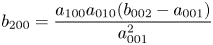

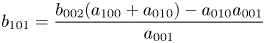
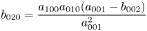
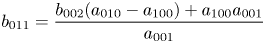
holds, then system (4.7) has a centre at the origin on the center manifold.
Proof. Observe that  $a_{001}=0$ is an elementary centre condition. Then, in this case, system (4.7) has a centre at the origin on the center manifold. This proves statement (a).
In what follows we will assume that  $a_{001}\neq 0$. We distinguish two cases
  $a_{100}=a_{010}=0$ and
  $a_{100}^{2}+a_{010}^{2}\neq 0$. If
  $a_{100}=a_{010}=0$, computing the first six focus quantities and using the computer algebra system Singular, we obtain the decomposition of the radical of the ideal generated by these focus quantities
  $I=\langle g_{220}, \ldots , g_{770} \rangle$ into an intersection of prime ideals. This decomposition consists of the following four ideals
 \begin{align*} I_1 &= \langle a_{001} \rangle, \;\; I_2=\langle b_{200}, b_{110}, b_{020}\rangle, \;\; I_3= \langle b_{200}+ b_{020}, 2a_{001}-b_{002}, b_{101}, b_{011}\rangle,\\ I_4 & = \langle b_{200}+ b_{020}, b_{101}^{2} + b_{011}^{2}, b_{110}^{2} +4 b_{020}^{2}, b_{110}b_{101} + 2b_{020}b_{011}, b_{110}b_{011} - 2b_{101}b_{020}\rangle. \end{align*}
Studying the zeros of the generators from above ideals, we obtain the four set of zeros  $\{a_{001}=0\}$,
  $\{b_{200}=b_{110}=b_{020}=0\}$,
  $\{b_{101}=b_{011}=0, b_{002}=2a_{001}, b_{020}=-b_{200}\}$ and
  $\{b_{200}=b_{110}=b_{101}=b_{020}=b_{011}=0\}$. Note that
  $b_{200}=b_{110}=b_{020}=0$ is an elementary centre condition and so, in this case, system (4.7) has a centre at the origin on the center manifold. As
  $a_{001}\neq 0$, remains to check the condition
  $b_{101}=b_{011}=0, b_{002}=2a_{001}$, and
  $b_{020}=-b_{200}$. Denote by
  $X$ the vector field associated with system (4.7) in this case. We have that
  $Xf=kf$, where
  $Xf=\langle X, \nabla f\rangle$,
  $f(x, y, z)=z-h(x, y)$,
  $k(x, y, z)=2a_{001}-1$, and
 \[ h(x, y)=\dfrac{1}{5}\, ( { b_{200}}-{ b_{110} }) {x}^{2}+\dfrac{1}{5}\, ( 4\,{ b_{200}}+{ b_{110}} ) xy+\dfrac{1}{5}\, ( { b_{110}}-{ b_{200}} ) {y}^{2}. \]
Therefore,  $f=0$ is an invariant algebraic surface of
  $X$ and
  $k$ is its cofactor (see p. 215 from [Reference Dumortier, Llibre and Artés13]). Note that the plane
  $xy$ is the tangent plane of
  $f=0$ at the origin and so the center manifold is given by the graphic of
  $z=h(x, y)$. Hence, denoting by
  $X\mid _{z=h(x, y)}$ the vector field
  $X$ restricted your center manifold at the origin (i.e.
  $X\mid _{z=h(x, y)}$ is obtained substituting
  ${z=h(x, y)}$ in the first two equations of (4.7)), we have that
  $(X\mid _{z=h(x, y)})V=(\mbox {div}\; X\mid _{z=h(x, y)} )\;V$, where
 \[ \begin{aligned} V(x, y) & = {{ a_{001}}}^{2} ( 4\,{ b_{200}}+{ b_{110}} ) ^{2}{x}^{4}-4\,{{ a_{001}}}^{2} ( { b_{200}}-{ b_{110}} ) ( 4\,{ b_{200}}+{ b_{110}} ) {x}^{3}y\\ & \quad+4\,{{ a_{001}}}^{2} ( { b_{200}}-{ b_{110}} ) ^{2}{x}^{2}{y}^{2}-10\,{ a_{001}}\, ( 4\,{ b_{200}}+{ b_{110}} ) {x}^{2}\\ & \quad+20\,{ a_{001}}\, ( { b_{200}}-{ b_{110}} ) xy+25. \end{aligned} \]
Thus  $V$ is an inverse integrate factor of
  $X\mid _{z=h(x, y)}$ and as
  $V(0,0)\neq 0$, it follows that the origin is a centre of
  $X\mid _{z=h(x, y)}$, i.e. the origin is a centre on the center manifold of system (4.7) in this case (see [Reference García and Grau17] for more details). This concludes the proof of statement (c).
If  $a_{100}^{2}+a_{010}^{2}\neq 0$, doing the change of variables (4.4), we can write system (4.7) with
  $F_1=\tilde F_1$ and
  $R_2=\tilde R_2$, where
  $\tilde F_1(x, y, z)=y+z$ and
  $\tilde R_2(x, y, z)=\tilde b_{200}x^{2}+\tilde b_{110}xy+\tilde b_{101}xz+\tilde b_{020}y^{2}+\tilde b_{011}yz+\tilde b_{002}z^{2}$. The expression of the
  $\tilde b_{ijk}$ are omitted for simplicity. In this case the first focus quantities is
  $g_{220}= \tilde b_{200} + \tilde b_{020}$. Thus, we have
  $\tilde b_{020}=-\tilde b_{200}$ and even calculating the next nine focus quantities, we were unable to obtain the necessary and sufficient conditions to have a centre on the center manifold. However, using the computer algebra system Singular, we obtain the decomposition over a field of characteristic 32 003 of the radical of the ideal generated by the next six focus quantities
  $\tilde I=\langle g_{330}, \ldots , g_{770} \rangle$ into an intersection of prime ideals. This decomposition consists of the following six ideals:
 \begin{align*} \tilde I_1 &= \langle \tilde b_{101}^{2} + \tilde b_{011}^{2} - 2\tilde b_{101} - 4\tilde b_{011} + 5, \; 16\,001\tilde b_{110}\tilde b_{101} + \tilde b_{200}\tilde b_{011} - 2\tilde b_{200}\\ &\quad - 16\,001\tilde b_{110},\; \tilde b_{200}\tilde b_{101} - 16\,001\tilde b_{110}\tilde b_{011} - \tilde b_{200} - \tilde b_{110}, \; \tilde b_{200}^{2} + 8001\tilde b_{110}^{2}\rangle,\\ \tilde I_2&= \langle \tilde b_{101}^{2} + \tilde b_{011}^{2} - 2\tilde b_{101} - 6\tilde b_{011} + 10, \; 16\,001\tilde b_{110}\tilde b_{101} + \tilde b_{200}\tilde b_{011} - 3\tilde b_{200}\\ &\quad - 16\,001\tilde b_{110}, \tilde b_{200}\tilde b_{101} - 16001\tilde b_{110}\tilde b_{011} - \tilde b_{200} + 16\,000\tilde b_{110}, \; \tilde b_{200}^{2} + 8001\tilde b_{110}^{2}\rangle,\\ \tilde I_3 &= \langle \tilde b_{200}, \tilde b_{110}\rangle,\; \tilde I_4= \langle \tilde b_{101}-, \tilde b_{011}-2, \tilde b_{002}-2\rangle,\\ \tilde I_5&= \langle \tilde b_{200}-\tilde b_{110}, \tilde b_{101}, \tilde b_{011}-2, \tilde b_{002}-2\rangle,\\ \tilde I_6 & = \langle \tilde b_{200}, \tilde b_{110}-\tilde b_{002}+1,\tilde b_{101}-\tilde b_{002}+1, \tilde b_{011}-\tilde b_{002}\rangle. \end{align*}
Here  $8001\equiv 1/4$ (mod 32 003) ,
  $16\,000\equiv -3/2$ (mod 32 003), and
  $16\,001\equiv -1/2$ (mod 32 003). The set of zeros of the generators of
  $\tilde I_3$ is
 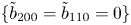 $\{\tilde b_{200}=\tilde b_{110}=0\}$. Hence, as in the previous case,
 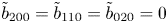 $\tilde b_{200}=\tilde b_{110}=\tilde b_{020}=0$ implies that system (4.7) has a centre at the origin on the center manifold. This concludes the proof of statement (b).
Studying the set of zeros from other ideals above, we obtain the following sets of conditions
(i)
$\tilde b_{020}=-\tilde b_{200}$, $\tilde b_{101}=1$, $\tilde b_{011}=\tilde b_{002}=2$,(ii)
$\tilde b_{020}=-\tilde b_{200}$, $\tilde b_{110}=\tilde b_{200}$, $\tilde b_{101}=0$, $\tilde b_{011}=\tilde b_{002}=2$,(iii)
$\tilde b_{020}=-\tilde b_{200}$, $\tilde b_{200}=\tilde b_{020}=0$, $\tilde b_{101}=\tilde b_{110}=\tilde b_{002}-1$, $\tilde b_{011}=\tilde b_{002}$.


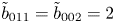


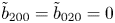


Conditions (i), (ii) and (iii) correspond to conditions (d), (e) and (f) from proposition, on the set of the original parameters, respectively.
Consider system (4.7) with  $F_1=\tilde F_1$,
  $R_2=\tilde R_2$, and condition (i). In this case system (4.7) has two invariant algebraic surfaces
  $f_1=0$ and
  $f_2=0$, where
  $f_1(x, y, z)=x^{2}+y^{2}$,
  $f_2(x, y, z)=( 1-\tilde b_{110}) x^{2}+2\tilde b_{200}xy-2x-2z+1$, and
  $k(x, y, z)=2y+2z$ is the cofactor of both curves. Therefore,
  $H=f_1/f_2$ is a first integral of system (4.7), i.e.
  $XH\equiv 0$, where
  $X$ denotes the vector field associated with the system (see p. 219 of [Reference Dumortier, Llibre and Artés13] for more details). Moreover, the Taylor series of
  $H$ in the origin has the form
 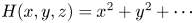 $H(x, y, z)=x^{2}+y^{2}+\cdots$. So, by theorem
  $3$ of [Reference Edneral, Mahdi, Romanovski and Shafer14] (see also [Reference Bibikov2]), we have a centre at the origin on the center manifold. This proves statement (d).
Now for system (4.7) with  $F_1=\tilde F_1$,
  $R_2=\tilde R_2$, and satisfying condition (ii) the associated vector field
  $X$ has an invariant algebraic surface given by
  $f(x, y, z)=z-h(x, y)$ with cofactor
  $k(x, y, z)=2y+2z-1$, where
  $h(x, y)=\tilde b_{200}xy$. As the plane
  $xy$ is the tangent plane of
  $f=0$ at the origin, it follows that the center manifold is given by the graphic of
  $z=h(x, y)$. Hence, denoting by
  $X\mid _{z=h(x, y)}$ the vector field
  $X$ restricted your center manifold at the origin, we have that the planar system associated with
  $X\mid _{z=h(x, y)}$ is invariant by the change of variables
  $(x, y,t)\mapsto (x,-y,-t)$. i.e.
  $X\mid _{z=h(x, y)}$ is reversible. Therefore, we have a centre at the origin on the center manifold, what proves statement (e).
Finally, consider system (4.7) with  $F_1=\tilde F_1$,
  $R_2=\tilde R_2$, and condition (iii). First we suppose that
  $b_{002}\neq 0$. In this case system (4.7) has two invariant algebraic surfaces,
  $f_1=0$ and
  $f_2=0$, where
  $f_1(x, y, z)=x^{2}+y^{2}$ and
  $f_2(x, y, z)=-b_{002} x-b_{002}z+1$ with respective cofactors
  $k_1(x, y, z)=2y+2z$ and
  $k_2(x, y, z)=b_{002}y+b_{002}z$. Therefore,
  $H=f_1/(f_2)^{(2/b_{002})}$ is a first integral of system (4.7). If
  $b_{002}= 0$, as in the previous case, system (4.7) has the invariant algebraic surface,
  $f_1=0$ and an exponential factor
  $g(x, y, z)=\textrm {e}^{2x+2y}$ (see p. 217 of [Reference Dumortier, Llibre and Artés13]), with respective cofactors
  $k_1$ and
  $k_g=-k_1$. Therefore,
  $G=f_1g$ is a first integral of system (4.7). Moreover, the Taylor series of
  $H$ and
  $G$ in the origin has the form
  $x^{2}+y^{2}+\cdots$. As in the previous case, we have a centre at the origin on the center manifold. This proves statement (f) and complete the proof of proposition.
Another interesting class of homogeneous rigid systems in  $\mathbb {R}^{3}$ are the systems of the form (3.1) with
  $n=m$ and
  $F_m=R_n$. In the next theorem we consider the case
  $m=2$. Observe that the centre conditions are only the elementary.
Theorem 4.4 Consider system (3.1) with  $n=m=2$,
  $\lambda =1$ and
  $F_2=R_2$, i.e. system
 \begin{equation} \dot x ={-} y + x F_2(x, y, z), \;\; \dot y = x+ yF_2(x, y, z), \;\; \dot z ={-} z + F_2(x, y, z), \end{equation}
where  $F_1(x, y, z)=a_{200}x^{2}+a_{110}xy+a_{101}xz+a_{020}y^{2}+a_{011}yz+a_{002}z^{2}$. Then system (4.8) has a centre at the origin on the center manifold if and only if one of the following conditions
(a)
$a_{200}=a_{110}=a_{020}=0$,(b)
$a_{020}=-a_{200}$ and $a_{101}=a_{011}=a_{002}=0$,

holds.
Proof. Computing the first six focus quantities and using the computer algebra system Singular, we obtain the decomposition of the radical of the ideal generated by the six focus quantities  $I=\langle g_{220}, \ldots , g_{770} \rangle$ into an intersection of prime ideals. This decomposition consists of the following three ideals
 \begin{align*} I_1 & = \langle a_{200} + a_{020}, a_{110}, a_{020}\rangle,\; I_2=\langle a_{200} + a_{020}, a_{101}, a_{011}, a_{002}\rangle,\\ I_3 & = \langle a_{200} + a_{020}, a_{101}^{2} + a_{011}^{2}, a_{110}^{2} + 4a_{020}^{2}, a_{110}a_{101}\\ & \quad + 2a_{020}a_{011}, -2a_{101}a_{020} + a_{110}a_{011}\rangle. \end{align*}
Note that the conditions of statements (a) and (b) belong to the set of zeros of the generators from above ideals. Therefore, they are necessary for the origin to be a centre of system (4.8) on the center manifold. Now, by the propositions 3.1 and 3.2 they are also sufficient.
5. Centre problem for some classes of non-homogeneous rigid systems in $ {\mathbb {R}}^{3}$

In this section we consider some systems of the form (2.7) where  $F$ is a polynomial in the variable
  $z$ and
  $R$ is a homogenous polynomial in three or two variables. Observe that if
  $z$ is a common factor of
  $R$ or
  $F\equiv 0$ we have that the origin is a centre on the center manifold. In this case we call this conditions of elementary centre conditions for these systems. The study of this type of systems was motivated by general results obtained for some families of rigid systems in the plane, i.e. systems of the form (2.2) such that
  $F$ is a polynomial of one variable or product of polynomials of one variable. More precisely, in [Reference Dias and Mello12, Reference Llibre and Rabanal28] the authors obtain a very simple bases for the ideal generated by the focal quantities.
Theorem 5.1 Consider system
 \begin{equation} \dot x ={-} y + x F(z), \;\; \dot y = x+ y F(z), \;\; \dot z ={-} z + R_2(x, y, z). \end{equation}
where  $F(z)=\sum _{j=1} ^{9}a_{j} z^{j}$ and
  $R_2(x, y, z)=b_{200}x^{2}+b_{110}xy+b_{101}xz+b_{020}y^{2}+b_{011}yz+b_{002}z^{2}$.
(a) Assume that
$a_2=a_4=a_5=\cdots =a_9=0$ (i.e. $F(z)=a_{1}z+a_{3}z^{3}$), then system (5.1) has a centre at the origin on the center manifold if and only if either $a_1=a_3=0$ or $b_{200}=b_{110}=b_{020}=0$ or $b_{101}=b_{011}=a_3=0$, $b_{002}=2a_{1}$, and $b_{020}=-b_{200}$.(b) Assume that
$a_1=a_3=a_5=a_7=a_9=0$ (i.e. $F(z)$ is an even function), then system (5.1) has a centre at the origin on the center manifold if and only if either $a_2=a_4=a_6=a_8=0$ or $b_{200}=b_{110}=b_{020}=0$.(c) Assume that
$b_{110}=b_{020}=b_{011}=0$ (i.e. $R_2(x, y, z)=R_2(x,z)$ is a homogeneous polynomial of degree 2 on the variables $x$, $z$), then system (5.1) has a centre at the origin on the center manifold if and only if either $a_1=\cdots =a_9=0$ or $b_{200}=0$.(d) Assume that
$a_5=\cdots =a_9=0$ and $b_{101}=b_{011}=b_{002}=0$ (i.e. $F(z)=a_{1}z+a_{2}z^{2}+a_{3}z^{3}+a_{4}z^{4}$ and $R_2(x, y, z)=R_2(x, y)$ is a homogeneous polynomial of degree 2 on the variables $x$, $y$), then system (5.1) has a centre at the origin on the center manifold if and only if either $a_1=a_2=a_3=a_4=0$ or $b_{200}=b_{110}=b_{020}=0$.


Proof. To prove statement (a) we distinguish two cases,  $b_{101}=b_{011}=0$ and
  $b_{101}^{2}+b_{011}^{2}\neq 0$. In the first case, we have that the decomposition of the radical of the ideal generated by the six focus quantities
  $I=\langle g_{220}, \ldots , g_{770} \rangle$, into an intersection of prime ideals, consists of the following three ideals
 \[ \begin{aligned} I_1= & \langle a_{1} , a_{3}\rangle,\; I_2=\langle b_{200} + b_{020}, b_{110}^{2}+ 4b_{020}^{2}\rangle,\; I_3= \langle a_{3}, 2a_{1}-b_{002}, b_{200} + b_{020} \rangle. \end{aligned} \]
The conditions  $\{ a_1=a_3=0\}$,
  $\{b_{200}=b_{110}=b_{020}=0\}$ and
  $\{a_3=0, b_{002}=2a_{1}, b_{020}=-b_{200}\}$ correspond to the set of zeros of the generators from above ideals. Therefore, they are necessary for the origin to be a centre of system (5.1) on the center manifold. Now,
  $\{ a_1=a_3=0\}$ and
  $\{b_{200}=b_{110}=b_{020}=0\}$ are also sufficient because they are elementary centre conditions. Note that system (5.1) with the condition
  $\{a_3=0, b_{002}=2a_{1}, b_{020}=-b_{200}\}$ is exactly system (4.7) with the condition (c) of theorem 4.3. Therefore, this condition is also sufficient.
When  $b_{101}^{2}+b_{011}^{2}\neq 0$, we can assume that
  $b_{101}=b_{011}=1$. Otherwise, we do the change of variables
 \[ x = \frac{b_{101}+b_{011}}{b_{101}^{2}+b_{011}^{2}}X+ \frac{b_{101}-b_{011}}{b_{101}^{2}+b_{011}^{2}}Y, \;\; y ={-}\frac{b_{101}-b_{011}}{b_{101}^{2}+b_{011}^{2}}X+ \frac{b_{101}+b_{011}}{b_{101}^{2}+b_{011}^{2}}Y, \;\; z = Z. \]
In this case, the decomposition of the radical of the ideal generated by the seven focus quantities 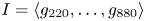 $I=\langle g_{220}, \ldots , g_{880} \rangle$, into an intersection of prime ideals, consists of the two ideals
 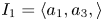 $I_1= \langle a_{1} , a_{3},\rangle$ and
 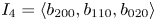 $I_4=\langle b_{200}, b_{110}, b_{020}\rangle$. As in the previous case, we have that the origin is a centre on the center manifold.
With the hypothesis of statement (b) we can suppose that  $b_{020}=b_{200}$ in system (5.1), otherwise we do the following change of variables
 \[ \begin{aligned} & x =(b_{200}-b_{020})X-(b_{110}+\sqrt{(b_{200}-b_{020})^{2}+b_{110}^{2}})Y,\\ & y = (b_{110}+\sqrt{(b_{200}-b_{020})^{2}+b_{110}^{2}})X+ (b_{200}-b_{020})Y,\\ & z = Z. \end{aligned} \]
In this case we have that the two first focus quantities are  $g_{220}=0$ and
 \[ g_{330}=\dfrac{1}{20} a_2 (40 b_{200}^{2}+b_{110}^{2}). \]
If  $a_2\neq 0$, then we must have
  $b_{200}=b_{110}=0$. Hence, we have an elementary centre condition and so the origin is a centre on the center manifold. Now, if
  $a_2=0$, the next two focus quantities are
  $g_{440}=0$ and
 \[ g_{550}=a_4 \Bigg(2 b_{200}^{4}+\dfrac{3 b_{200}^{2} b_{110}^{2}}{10}+\dfrac{3 b_{110}^{4}}{1600}\Bigg). \]
Therefore, we must have  $a_4=0$ and the next focus quantities is
 \[ g_{660}=a_6 \Bigg(2 b_{200}^{6}+\dfrac{3 b_{200}^{4} b_{110}^{2}}{4}+\dfrac{9 b_{200}^{2} b_{110}^{4}}{320}+\dfrac{b_{110}^{6}}{12800}\Bigg). \]
Hence, we have that  $a_6=0$ and the next two focus quantities are
  $g_{770}=0$ and
 \[ g_{880}=a_8 \Bigg(2 b_{200}^{8}+\dfrac{7 b_{200}^{6} b_{110}^{2}}{5}+\dfrac{21 b_{200}^{4} b_{110}^{4}}{160}+\dfrac{7 b_{200}^{2} b_{110}^{6}}{3200}+\dfrac{7 b_{110}^{8}}{2048000}\Bigg). \]
We must have  $a_8=0$ and so the origin is a centre on the center manifold, because we have an elementary centre condition.
Now we will prove statement (c) of theorem. Computing the first nine focus quantities  $g_{kk0}$,
  $k=2, \ldots , 10$, we have that the Groebner basis of ideal generated by these quantities is given by
  $\{a_j(b_{200})^{j}\}_{j=1,\ldots , 9}$. Therefore, it follows that the origin is a centre on the center manifold if only if
  $b_{200}=0$ or
  $a_1=\cdots =a_9=0$, because these conditions are the elementary centre conditions.
Finally, we will prove statement (d) of theorem. The decomposition of the radical of the ideal generated by the eight focus quantities 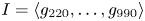 $I=\langle g_{220}, \ldots , g_{990} \rangle$, into an intersection of prime ideals, consists of the two ideals
  $I_1= \langle a_{1} , a_{2}, a_{3}, a_{4}\rangle$ and
  $I_2=\langle b_{200}+b_{020}, b_{110}^{2}+4b_{020}\rangle$. Again we have only elementary centre conditions and so the origin is a centre on the center manifold.
Statement (c) of theorem 5.1 lead us to the conjecture that if in system (2.7)  $F$ is given by
  $F(z)=\sum _{j=1} ^{n}a_{j} z^{j}$, and
  $R$ is given by
  $R(x,z)=\sum _{j+k=2} b_{jk} x^{j}z^{k}$, then a basis to ideal generated by its focus quantities is
  $\{a_j(b_{20})^{j}\}_{j=1,\ldots , n}$.
Observe that in the proof of statements (b), (c) and (d) we have only elementary centre conditions. In statement (a) we have one centre conditions that is not elementary. In the next result we have another family of rigid systems with one non elementary centre conditions, even with  $R$ a homogeneous polynomial in two variables.
Theorem 5.2 Consider system (2.7) with  $F$ and
  $R$ given by
  $F(z)=a_{1}z+a_{2}z^{2}+a_{3}z^{3}$ and
  $R(x,z)=\sum _{j+k=3} b_{jk} x^{j}z^{k}$. Then the origin is a centre on the center manifold if and only if either
  $a_1=a_2=a_3=0$ or
  $b_{30}=0$ or
  $a_2=3 a_1^{2}$,
  $a_3=0$,
  $b_{21}=b_{12}=0$ and
  $b_{03}=9a_{1}^{2}$.
Proof. We have that  $g_{220}=0$ and the decomposition of the radical of the ideal generated by the next ten focus quantities
  $I=\langle g_{kk0} \rangle _{k=3, \ldots , 13}$, into an intersection of prime ideals, consists of the three ideals
  $I_1= \langle a_{1} , a_{2}, a_{3}\rangle$,
  $I_2=\langle b_{30}\rangle$ and
  $I_3=\langle 9 a_1^{2}-b_{03}, a_3, b_{21}, b_{12}, 3 a_2-b_{03}\rangle$. The conditions
  $\{a_1=a_2=a_3=0\}$,
  $\{b_{30}=0\}$ and
  $\{a_2=3 a_1^{2}, a_3=0, b_{21}=b_{12}=0, b_{03}=9a_{1}^{2}\}$ correspond to the set of zeros of the generators from above ideals. Note that the two first conditions are elementary centre conditions and so we have a centre at the origin on the center manifold. For the last condition, note that
  $f_{1}(x, y, z)=x^{2}+y^{2}$ and
  $f_2(x, y, z)=3 a_1b_{30}x^{2} y+2 a_1 b_{30} y^{3}-3 a_1 z+1$ are invariant algebraic surfaces of system with the cofactors
  $k_1(x, y, z)=6 a_1^{2} z^{2}+2a_1 z$ and
  $k_2(x, y, z)=9 a_1^{2} z^{2}+3a_1 z$, respectively. Hence,
  $H=f_1 f_2^{-2/3}$ is a first integral of system and the Taylor series of
  $H$ in the origin has the form
  $x^{2}+y^{2}+\cdots$. Therefore, we have a centre at the origin on the center manifold.
Acknowledgements
The second author is partially supported by São Paulo Research Foundation (FAPESP) grants 18/19726-5 and 19/10269-3 and by CAPES PROCAD grant 88881.068462/2014-01. The third author is partially supported by the Instituto Federal de Educação, Ciência e Tecnologia do Sul de Minas Gerais - IFSULDEMINAS.


