


1 Introduction
When a thin liquid film is coated on the surface of a fibre, it will undergo capillary instability (Bretherton Reference Bretherton1961; Kalliadasis & Chang Reference Kalliadasis and Chang1994; Kliakhandler, Davis & Bankoff Reference Kliakhandler, Davis and Bankoff2001; Craster & Matar Reference Craster and Matar2006; Ruyer-Quil et al. Reference Ruyer-Quil, Treveleyan, Giorgiutti-Dauphiné, Duprat and Kalliadasis2008; Kalliadasis et al. Reference Kalliadasis, Ruyer-Quil, Scheid and Velarde2011). This instability is driven by surface tension and mainly arises from the circumferential curvature of the interface. Specifically, inevitable interfacial fluctuations will cause the circumferential Laplace pressures in the valleys to be higher than those in the troughs. As a result, the fluid in the valleys will be sucked toward the troughs, thereby amplifying the fluctuations and eventually making the film grow into large drops. If the fibre is placed in a vertical arrangement, capillary instability still persists. However, because of gravity, a drop gains (loses) an additional mass flow from the film behind (ahead of) the drop as it travels down the fibre (see figure 1). This continuous mass flow injection/ejection due to gravity will compete with the capillary flow due to surface tension, consequently affecting the resulting drop profile and travelling speed. This fibre coating problem has been studied both theoretically (Kalliadasis & Chang Reference Kalliadasis and Chang1994; Yu & Hinch Reference Yu and Hinch2013) and experimentally (Quéré Reference Quéré1990), so the basic physics can be said to be well understood. However, there still exists a noticeable discrepancy between experiment and theory. This motivates us to revisit this problem to seek a plausible explanation to resolve this discrepancy. To see how the problem is motivated, we first look at experimental observations. Quéré (Reference Quéré1990) conducted an experiment and found that such a flow can behave quite differently, depending on the film thickness. If the film is sufficiently thick, it will grow into bulges and turn into large drops. On the other hand, if the film thickness is below some critical value, bulges will be suppressed and maintain a steady shape. In other words, the film’s growth can be inhibited by the saturation of the capillary instability. As the film thickness controls the relative importance between surface tension and gravitational forces, the Bond number characterizes the flow behaviour,
 $$\begin{eqnarray}G=\frac{\unicode[STIX]{x1D70C}ga^{3}}{\unicode[STIX]{x1D6FE}h_{0}},\end{eqnarray}$$
where
 $\unicode[STIX]{x1D70C}$
is the fluid density,
$\unicode[STIX]{x1D70C}$
is the fluid density,
 $g$
is the gravitational acceleration,
$g$
is the gravitational acceleration,
 $a$
is the fibre radius,
$a$
is the fibre radius,
 $\unicode[STIX]{x1D6FE}$
is the surface tension and
$\unicode[STIX]{x1D6FE}$
is the surface tension and
 $h_{0}$
is the unperturbed film thickness. This dimensionless parameter can also be recognized as the velocity ratio of gravity-driven flow
$h_{0}$
is the unperturbed film thickness. This dimensionless parameter can also be recognized as the velocity ratio of gravity-driven flow
 $\unicode[STIX]{x1D70C}gh_{0}^{2}/\unicode[STIX]{x1D707}$
to capillary flow
$\unicode[STIX]{x1D70C}gh_{0}^{2}/\unicode[STIX]{x1D707}$
to capillary flow
 $(h_{0}/a)^{3}(\unicode[STIX]{x1D6FE}/\unicode[STIX]{x1D707})$
, with
$(h_{0}/a)^{3}(\unicode[STIX]{x1D6FE}/\unicode[STIX]{x1D707})$
, with
 $\unicode[STIX]{x1D707}$
being the fluid viscosity. As can be seen from (1.1), for given fluid and fibre radius, the unperturbed film thickness
$\unicode[STIX]{x1D707}$
being the fluid viscosity. As can be seen from (1.1), for given fluid and fibre radius, the unperturbed film thickness
 $h_{0}$
controls the magnitude of
$h_{0}$
controls the magnitude of
 $G$
critical to the dynamics of the film. For thick films such that
$G$
critical to the dynamics of the film. For thick films such that
 $G$
is small, surface tension dominates over gravity, thereby giving rise to drop formation due to capillary instability. On the other hand, if
$G$
is small, surface tension dominates over gravity, thereby giving rise to drop formation due to capillary instability. On the other hand, if
 $G$
is large when the film is sufficiently thin, the much stronger gravity force suppresses the capillary instability, thereby making the interface slightly undulated and advected with the falling flow. Hence, drop formation occurs if
$G$
is large when the film is sufficiently thin, the much stronger gravity force suppresses the capillary instability, thereby making the interface slightly undulated and advected with the falling flow. Hence, drop formation occurs if
 $G$
is smaller than some critical value
$G$
is smaller than some critical value
 $G_{c}$
. Quéré (Reference Quéré1990) found
$G_{c}$
. Quéré (Reference Quéré1990) found
 $G_{c}\approx 0.71$
. Similar drop formation and suppression can also occur to a pressure-driven core annular film flow where the behaviour of the interface is determined by the competition between surface tension and shear flow effects within the film (Kerchman Reference Kerchman1995).
$G_{c}\approx 0.71$
. Similar drop formation and suppression can also occur to a pressure-driven core annular film flow where the behaviour of the interface is determined by the competition between surface tension and shear flow effects within the film (Kerchman Reference Kerchman1995).

Figure 1. Sketch of a liquid film flowing down a slippery fibre of radius
 $a$
and slip length
$a$
and slip length
 $\unicode[STIX]{x1D706}$
. Owing to interplays between capillary suction and gravity draining, the film thickness
$\unicode[STIX]{x1D706}$
. Owing to interplays between capillary suction and gravity draining, the film thickness
 $h(x,t)$
can vary with the axial position
$h(x,t)$
can vary with the axial position
 $x$
and time
$x$
and time
 $t$
. Here
$t$
. Here
 $h_{0}$
is the unperturbed film thickness and
$h_{0}$
is the unperturbed film thickness and
 $g$
is the gravitational acceleration. In terms of dimensionless variables throughout this work,
$g$
is the gravitational acceleration. In terms of dimensionless variables throughout this work,
 $x$
and the transverse position
$x$
and the transverse position
 $y$
are scaled by
$y$
are scaled by
 $a$
and
$a$
and
 $h_{0}$
, respectively, and
$h_{0}$
, respectively, and
 $t$
is scaled by
$t$
is scaled by
 $3\unicode[STIX]{x1D707}a^{4}/\unicode[STIX]{x1D6FE}h_{0}^{3}$
.
$3\unicode[STIX]{x1D707}a^{4}/\unicode[STIX]{x1D6FE}h_{0}^{3}$
.
On the theoretical side, the common approach to modelling this fibre coating problem is by solving lubrication-type interfacial evolution equations. There are extensive studies along this line, showing that most features of this problem can be successfully captured by this method (Frenkel Reference Frenkel1992; Kalliadasis & Chang Reference Kalliadasis and Chang1994; Kerchman & Frenkel Reference Kerchman and Frenkel1994; Kerchman Reference Kerchman1995; Chang & Demekhin Reference Chang and Demekhin1999; Kliakhandler et al.
Reference Kliakhandler, Davis and Bankoff2001; Duprat et al.
Reference Duprat, Ruyer-Quil, Kalliadasis and Giorgiutti-Dauphine2007; Ruyer-Quil et al.
Reference Ruyer-Quil, Treveleyan, Giorgiutti-Dauphiné, Duprat and Kalliadasis2008; Yu & Hinch Reference Yu and Hinch2013). Here we are more concerned with the critical Bond number
 $G_{c}$
for an onset of drop formation. Kalliadasis & Chang (Reference Kalliadasis and Chang1994) first predicted
$G_{c}$
for an onset of drop formation. Kalliadasis & Chang (Reference Kalliadasis and Chang1994) first predicted
 $G_{c}\approx 0.60$
using a matched asymptotic theory. Yu & Hinch (Reference Yu and Hinch2013) recently refined this result by including further corrections. In comparison,
$G_{c}\approx 0.60$
using a matched asymptotic theory. Yu & Hinch (Reference Yu and Hinch2013) recently refined this result by including further corrections. In comparison,
 $G_{c}\approx 0.71$
found by Quéré (Reference Quéré1990) is actually 18 % greater than the theoretical prediction
$G_{c}\approx 0.71$
found by Quéré (Reference Quéré1990) is actually 18 % greater than the theoretical prediction
 $G_{c}\approx 0.60$
. Although this discrepancy does not seem serious, it is nevertheless not unnoticeable. As the discrepancy here seems unlikely attributed to the lubrication model usually adopted, it could be that part of the inherent assumptions made in theory do not correspond to what happens in Quéré’s experiment.
$G_{c}\approx 0.60$
. Although this discrepancy does not seem serious, it is nevertheless not unnoticeable. As the discrepancy here seems unlikely attributed to the lubrication model usually adopted, it could be that part of the inherent assumptions made in theory do not correspond to what happens in Quéré’s experiment.
To see how the discrepancy arises, it is necessary to re-examine Quéré’s experiment. He used silicone oil, a polymeric liquid that can exhibit considerable fluid slippage on a solid wall as it flows (de Gennes Reference de Gennes1985; Brochard-Wyart et al.
Reference Brochard-Wyart, de Gennes, Hervert and Redon1994). Together with the fact that the fibres here are made of nylon, which is hydrophobic, and could admit wall slip as well (due, for instance, to microbubbles trapped by surface microgrooves (Lauga, Brenner & Stone Reference Lauga, Brenner and Stone2007)), it is likely that wall slip effects might no longer be negligible as usually considered. Previous studies showed that a variety of interfacial flows with wall slip could behave quite differently than those based on the no-slip boundary condition (Liao, Li & Wei Reference Liao, Li and Wei2013; Li et al.
Reference Li, Liao, Wen and Wei2014; Liao et al.
Reference Liao, Li, Chang, Huang and Wei2014; Halpern, Li & Wei Reference Halpern, Li and Wei2015). In particular, in the related work by Liao et al. (Reference Liao, Li and Wei2013), the authors found that a core annular film flow in a horizontal tube, even with a fractional amount of wall slip, can exhibit greater capillary instability than the usual no-slip case (Hammond Reference Hammond1983), especially when capillary draining proceeds to the stage where the film becomes thinner than the slip length. Recently, Haefner et al. (Reference Haefner, Benzaquen, Baumchen, Salez, Peters, McGraw, Jacobs, Raphael and Dalnoki-Veress2015) experimentally examined the influence of slip on capillary instability of a thin liquid film on a horizontal fibre, showing that interfacial undulations with slip do grow faster than those without slip. These studies imply that a thin, uniformly undulated film on a fibre would grow into bigger drops if wall slip is present. In other words, wall slip would facilitate drop formation by making drops start to appear at thinner films, which in turn makes the actual value of
 $G_{c}$
greater than that without slip. This might explain why the experimental value
$G_{c}$
greater than that without slip. This might explain why the experimental value
 $G_{c}\approx 0.71$
measured by Quéré (Reference Quéré1990) is slightly greater than the theoretical value
$G_{c}\approx 0.71$
measured by Quéré (Reference Quéré1990) is slightly greater than the theoretical value
 $G_{c}\approx 0.6$
predicted by the usual no-slip model (Kerchman & Frenkel Reference Kerchman and Frenkel1994; Yu & Hinch Reference Yu and Hinch2013).
$G_{c}\approx 0.6$
predicted by the usual no-slip model (Kerchman & Frenkel Reference Kerchman and Frenkel1994; Yu & Hinch Reference Yu and Hinch2013).
Motivated by the above, we examine in this paper how wall slip influences drop formation and interfacial dynamics for the fibre-coating problem. As will be shown shortly, wall slip not only enhances capillary instability resulting in bigger drops, but also leads
 $G_{c}$
to increase with the amount of wall slip, making a falling liquid more susceptible to drop formation. We also find that even when slip effects are strong, it is still possible to prevent the film from growing to drops by saturating the capillary instability. In the following, we begin with the mathematical formation for this problem in § 2. In § 3, we derive new scalings for the strong slip situation in distinction to those for the no-slip case given by Yu & Hinch (Reference Yu and Hinch2013). These strong slip scalings are also confirmed numerically. The general impact of wall slip on drop formation is presented in § 4. Connections to experiments will be made in § 5, showing that the discrepancy between experiment (Quéré Reference Quéré1990) and theory (Kerchman & Frenkel Reference Kerchman and Frenkel1994; Yu & Hinch Reference Yu and Hinch2013) can be reasonably resolved by including additional slip effects.
$G_{c}$
to increase with the amount of wall slip, making a falling liquid more susceptible to drop formation. We also find that even when slip effects are strong, it is still possible to prevent the film from growing to drops by saturating the capillary instability. In the following, we begin with the mathematical formation for this problem in § 2. In § 3, we derive new scalings for the strong slip situation in distinction to those for the no-slip case given by Yu & Hinch (Reference Yu and Hinch2013). These strong slip scalings are also confirmed numerically. The general impact of wall slip on drop formation is presented in § 4. Connections to experiments will be made in § 5, showing that the discrepancy between experiment (Quéré Reference Quéré1990) and theory (Kerchman & Frenkel Reference Kerchman and Frenkel1994; Yu & Hinch Reference Yu and Hinch2013) can be reasonably resolved by including additional slip effects.
2 Problem formulation
We follow the analysis of Yu & Hinch (Reference Yu and Hinch2013) in deriving an evolution equation for the thickness of the liquid layer coating a vertical fibre of radius
 $a$
. In order to apply the lubrication approximation, it is assumed that the film thickness is much smaller than the fibre radius,
$a$
. In order to apply the lubrication approximation, it is assumed that the film thickness is much smaller than the fibre radius,
 $h^{\ast }\ll a$
, and that the change in thickness in the axial direction is also small,
$h^{\ast }\ll a$
, and that the change in thickness in the axial direction is also small,
 $|\unicode[STIX]{x2202}h^{\ast }/\unicode[STIX]{x2202}x^{\ast }|\ll 1$
. The reduced momentum and continuity equations are
$|\unicode[STIX]{x2202}h^{\ast }/\unicode[STIX]{x2202}x^{\ast }|\ll 1$
. The reduced momentum and continuity equations are
 $$\begin{eqnarray}\unicode[STIX]{x1D707}u_{y^{\ast }y^{\ast }}^{\ast }=p_{x^{\ast }}^{\ast }-\unicode[STIX]{x1D70C}g,\quad p_{y^{\ast }}^{\ast }=0,\quad u_{x^{\ast }}^{\ast }+v_{y^{\ast }}^{\ast }=0.\end{eqnarray}$$
Here
 $(u^{\ast },v^{\ast })$
are the axial and transverse components of velocity,
$(u^{\ast },v^{\ast })$
are the axial and transverse components of velocity,
 $p^{\ast }$
is the pressure, and
$p^{\ast }$
is the pressure, and
 $\unicode[STIX]{x1D707}$
and
$\unicode[STIX]{x1D707}$
and
 $\unicode[STIX]{x1D70C}$
are the viscosity and density, respectively. Along the fibre, at
$\unicode[STIX]{x1D70C}$
are the viscosity and density, respectively. Along the fibre, at
 $y^{\ast }=0$
, we apply the Navier slip and no-penetration conditions on the velocity field:
$y^{\ast }=0$
, we apply the Navier slip and no-penetration conditions on the velocity field:
 $$\begin{eqnarray}u^{\ast }=\unicode[STIX]{x1D706}u_{y^{\ast }}^{\ast },\quad v^{\ast }=0,\end{eqnarray}$$
where
 $\unicode[STIX]{x1D706}$
is the slip length. At the free surface,
$\unicode[STIX]{x1D706}$
is the slip length. At the free surface,
 $y^{\ast }=h^{\ast }(x^{\ast },t^{\ast })$
, the balances of normal and tangential stresses are
$y^{\ast }=h^{\ast }(x^{\ast },t^{\ast })$
, the balances of normal and tangential stresses are
 $$\begin{eqnarray}p^{\ast }=\unicode[STIX]{x1D6FE}\left(\frac{-h^{\ast }}{a}-h_{x^{\ast }x^{\ast }}\right)\end{eqnarray}$$
and
 $$\begin{eqnarray}\unicode[STIX]{x1D707}u_{y^{\ast }}^{\ast }=0.\end{eqnarray}$$
Note that just as in Yu & Hinch (Reference Yu and Hinch2013), we have dropped the constant pressure term contribution that comes from the transverse component in curvature in (2.3) since it does not affect fluid motion, and we have applied the thin film approximation to the curvature of the surface. The kinematic boundary condition can be written as
 $$\begin{eqnarray}h_{t^{\ast }}^{\ast }+Q_{x^{\ast }}^{\ast }=0,\end{eqnarray}$$
where
 $Q^{\ast }=\int _{0}^{h^{\ast }}u^{\ast }\,\text{d}y^{\ast }$
is the axial flow rate. After integrating the momentum equation (2.1) and applying the boundary conditions (2.2) and (2.4), the following expression for the axial component of velocity is obtained:
$Q^{\ast }=\int _{0}^{h^{\ast }}u^{\ast }\,\text{d}y^{\ast }$
is the axial flow rate. After integrating the momentum equation (2.1) and applying the boundary conditions (2.2) and (2.4), the following expression for the axial component of velocity is obtained:
 $$\begin{eqnarray}u^{\ast }=\frac{1}{\unicode[STIX]{x1D707}}\left(p_{x\ast }^{\ast }-\unicode[STIX]{x1D70C}g\right)\left[\frac{y^{\ast 2}}{2}-h^{\ast }y^{\ast }-\unicode[STIX]{x1D706}h^{\ast }\right].\end{eqnarray}$$
Thus,
 $$\begin{eqnarray}Q^{\ast }=\frac{1}{3\unicode[STIX]{x1D707}}\left(\unicode[STIX]{x1D70C}g-p_{x^{\ast }}^{\ast }\right)\left[h^{\ast 3}+3\unicode[STIX]{x1D706}h^{\ast 2}\right].\end{eqnarray}$$
As in Yu & Hinch (Reference Yu and Hinch2013), we introduce the following dimensionless variables:
 $$\begin{eqnarray}x=\frac{x^{\ast }}{a},\quad h=\frac{h^{\ast }}{h_{0}},\quad t=\frac{t^{\ast }}{\left(3\unicode[STIX]{x1D707}a^{4}/\unicode[STIX]{x1D6FE}h_{0}^{3}\right)},\quad p=\frac{p^{\ast }}{\unicode[STIX]{x1D6FE}h_{0}/a^{2}},\end{eqnarray}$$
where
 $h_{0}$
is the unperturbed film thickness. Thus, after substituting (2.3) and (2.7) in (2.5), and applying this non-dimensionalization, the kinematic boundary condition yields an evolution equation for the film thickness,
$h_{0}$
is the unperturbed film thickness. Thus, after substituting (2.3) and (2.7) in (2.5), and applying this non-dimensionalization, the kinematic boundary condition yields an evolution equation for the film thickness,
 $$\begin{eqnarray}h_{t}+\left[\left(h^{3}+\unicode[STIX]{x1D6EC}h^{2}\right)\left(G+h_{x}+h_{xxx}\right)\right]_{x}=0,\end{eqnarray}$$
where
 $\unicode[STIX]{x1D6EC}=3\unicode[STIX]{x1D706}/h_{0}$
is the slip parameter measuring the extent of wall slip relative to the unperturbed film thickness
$\unicode[STIX]{x1D6EC}=3\unicode[STIX]{x1D706}/h_{0}$
is the slip parameter measuring the extent of wall slip relative to the unperturbed film thickness
 $h_{0}$
. This equation has a travelling wave solution that can be determined by letting
$h_{0}$
. This equation has a travelling wave solution that can be determined by letting
 $x\rightarrow x-ct$
and
$x\rightarrow x-ct$
and
 $h(x,t)\rightarrow h(x-ct)$
, where
$h(x,t)\rightarrow h(x-ct)$
, where
 $c$
is the propagating speed of the wave. Substituting the latter into (2.9) and integrating once with the uniform film condition
$c$
is the propagating speed of the wave. Substituting the latter into (2.9) and integrating once with the uniform film condition
 $h\rightarrow 1$
as
$h\rightarrow 1$
as
 $x\rightarrow \pm \infty$
, we obtain the following third-order equation for
$x\rightarrow \pm \infty$
, we obtain the following third-order equation for
 $h$
:
$h$
:
 $$\begin{eqnarray}-\!c\left(h-1\right)+\left(h^{3}+\unicode[STIX]{x1D6EC}h^{2}\right)\left(G+h_{x}+h_{xxx}\right)=\left(1+\unicode[STIX]{x1D6EC}\right)G,\end{eqnarray}$$
with
 $$\begin{eqnarray}h\rightarrow 1\quad \text{as }x\rightarrow \pm \infty .\end{eqnarray}$$
Equations (2.10) and (2.11) constitute an eigenvalue problem for
 $c(G,\unicode[STIX]{x1D6EC})$
, which is solved numerically using an iterative procedure similar to that in Yu & Hinch (Reference Yu and Hinch2013). For completeness, some details of this method are provided in appendix A.
$c(G,\unicode[STIX]{x1D6EC})$
, which is solved numerically using an iterative procedure similar to that in Yu & Hinch (Reference Yu and Hinch2013). For completeness, some details of this method are provided in appendix A.
It is worth mentioning that as in Yu & Hinch (Reference Yu and Hinch2013), the drop here is chosen to have a fixed length
 $2\unicode[STIX]{x03C0}$
(in the units of the fibre radius
$2\unicode[STIX]{x03C0}$
(in the units of the fibre radius
 $a$
), corresponding to the critical wavelength according to capillary instability (Hammond Reference Hammond1983). Perhaps it is more appropriate to choose the most unstable wavelength
$a$
), corresponding to the critical wavelength according to capillary instability (Hammond Reference Hammond1983). Perhaps it is more appropriate to choose the most unstable wavelength
 $2^{3/2}\unicode[STIX]{x03C0}$
to be the drop length (Kalliadasis & Chang Reference Kalliadasis and Chang1994). Yu & Hinch (Reference Yu and Hinch2013) found no differences between these two choices in terms of results. Also given that slip length does not change these two characteristic wavelengths for capillary instability (Liao et al.
Reference Liao, Li and Wei2013), keeping the same drop length
$2^{3/2}\unicode[STIX]{x03C0}$
to be the drop length (Kalliadasis & Chang Reference Kalliadasis and Chang1994). Yu & Hinch (Reference Yu and Hinch2013) found no differences between these two choices in terms of results. Also given that slip length does not change these two characteristic wavelengths for capillary instability (Liao et al.
Reference Liao, Li and Wei2013), keeping the same drop length
 $2\unicode[STIX]{x03C0}$
should not change the features in the presence of wall slip.
$2\unicode[STIX]{x03C0}$
should not change the features in the presence of wall slip.
3 Weak slip versus strong slip
Prior to presenting the overall influence of wall slip on the fibre-coating problem in § 4, it is instructive to gain some insights by inspecting scalings for both weak slip and strong slip limits. The weak slip (
 $\unicode[STIX]{x1D6EC}\ll 1$
) limit recovers the no-slip results found previously (Yu & Hinch Reference Yu and Hinch2013). As will be shown below, how wall slip impacts drop formation is due to a length scale change of the short transition films that connect the uniform film to the main drop, as sketched in figure 2. This change will manifest most when slip effects are strong. Consequently, the scalings in the strong slip (
$\unicode[STIX]{x1D6EC}\ll 1$
) limit recovers the no-slip results found previously (Yu & Hinch Reference Yu and Hinch2013). As will be shown below, how wall slip impacts drop formation is due to a length scale change of the short transition films that connect the uniform film to the main drop, as sketched in figure 2. This change will manifest most when slip effects are strong. Consequently, the scalings in the strong slip (
 $\unicode[STIX]{x1D6EC}\gg 1$
) limit will be completely different from the no-slip ones, which will help explain the various features shown in § 4.
$\unicode[STIX]{x1D6EC}\gg 1$
) limit will be completely different from the no-slip ones, which will help explain the various features shown in § 4.

Figure 2. Sketch of main drop and two transition film regions.
3.1 Weak slip limit
In the weak slip (
 $\unicode[STIX]{x1D6EC}\ll 1$
) limit, equation (2.10) reduces to the no-slip form (Yu & Hinch Reference Yu and Hinch2013):
$\unicode[STIX]{x1D6EC}\ll 1$
) limit, equation (2.10) reduces to the no-slip form (Yu & Hinch Reference Yu and Hinch2013):
 $$\begin{eqnarray}-\!c\left(h-1\right)+G\left(h^{3}-1\right)+h^{3}\left(h_{x}+h_{xxx}\right)=0.\end{eqnarray}$$
Following the approach by Yu & Hinch (Reference Yu and Hinch2013), we inspect the behaviour of the solutions in the transition film regions and the main drop region.
The length scale
 $\ell$
of the transition films is determined by balancing the travelling term
$\ell$
of the transition films is determined by balancing the travelling term
 $ch$
to the axial interfacial curvature term
$ch$
to the axial interfacial curvature term
 $h^{3}h_{xxx}\sim h^{4}/\ell ^{3}$
. Because
$h^{3}h_{xxx}\sim h^{4}/\ell ^{3}$
. Because
 $h\sim O(1)$
, this balance yields
$h\sim O(1)$
, this balance yields
 $$\begin{eqnarray}\ell \sim c^{-1/3}.\end{eqnarray}$$
This length scale is essentially obtained in a way similar to that in the classical Landau–Levich–Bretherton problem (Landau & Levich Reference Landau and Levich1942; Bretherton Reference Bretherton1961). Rescaling
 $z=c^{1/3}(x-x_{0})$
, equation (3.1) becomes
$z=c^{1/3}(x-x_{0})$
, equation (3.1) becomes
 $$\begin{eqnarray}h_{zzz}=\frac{h-1}{h^{3}}-c^{-2/3}h_{z}+c^{-1}G\frac{1-h^{3}}{h^{3}}.\end{eqnarray}$$
Hence, at leading order, equation (3.3) is simply governed by the Bretherton equation (Bretherton Reference Bretherton1961).
When moving toward the main drop region, the axial interface curvature in the transition region
 $h_{xx}\sim \ell ^{-2}$
has to match that of the main drop:
$h_{xx}\sim \ell ^{-2}$
has to match that of the main drop:
 $h_{max}/L^{2}\sim h_{max}$
, giving
$h_{max}/L^{2}\sim h_{max}$
, giving
 $$\begin{eqnarray}h_{max}\sim c^{2/3}(\gg 1).\end{eqnarray}$$
So in the main drop region, rescaling the drop height
 $H=h/c^{2/3}$
with (3.4), equation (3.1) becomes
$H=h/c^{2/3}$
with (3.4), equation (3.1) becomes
 $$\begin{eqnarray}H_{x}+H_{xxx}=c^{-1}\left(H-c^{-2/3}\right)/H^{3}-c^{-2/3}G\left(1-c^{-2}/H^{3}\right).\end{eqnarray}$$
As a result, the leading term is the curvature term on the left-hand side, meaning that at leading order the pressure in the main drop remains hydrostatic (Hammond Reference Hammond1983).
3.2 Strong slip limit
When wall slip is present and the slip length is large compared with the film thickness, we again use the balance
 $ch\sim \unicode[STIX]{x1D6EC}h^{2}h_{xxx}\sim \unicode[STIX]{x1D6EC}h^{3}/\ell ^{3}$
to determine the length scale of the transition films as
$ch\sim \unicode[STIX]{x1D6EC}h^{2}h_{xxx}\sim \unicode[STIX]{x1D6EC}h^{3}/\ell ^{3}$
to determine the length scale of the transition films as
 $$\begin{eqnarray}\ell \sim {\hat{c}}^{-1/3},\end{eqnarray}$$
where
 ${\hat{c}}=c/\unicode[STIX]{x1D6EC}$
. So the equation governing the transition films can be obtained by rescaling (2.10) with
${\hat{c}}=c/\unicode[STIX]{x1D6EC}$
. So the equation governing the transition films can be obtained by rescaling (2.10) with
 $\unicode[STIX]{x1D701}={\hat{c}}^{1/3}(x-x_{0})$
:
$\unicode[STIX]{x1D701}={\hat{c}}^{1/3}(x-x_{0})$
:
 $$\begin{eqnarray}h_{\unicode[STIX]{x1D701}\unicode[STIX]{x1D701}\unicode[STIX]{x1D701}}=\frac{h-1}{h^{2}\left(1+\unicode[STIX]{x1D6EC}^{-1}h\right)}-{\hat{c}}^{-2/3}h_{\unicode[STIX]{x1D701}}+{\hat{c}}^{-1}G\left[\frac{1+\unicode[STIX]{x1D6EC}^{-1}}{h^{2}\left(1+\unicode[STIX]{x1D6EC}^{-1}h\right)}-1\right].\end{eqnarray}$$
For large
 $\unicode[STIX]{x1D6EC}$
, the leading order contribution in (3.7) is
$\unicode[STIX]{x1D6EC}$
, the leading order contribution in (3.7) is
 $h_{\unicode[STIX]{x1D701}\unicode[STIX]{x1D701}\unicode[STIX]{x1D701}}=(h-1)/h^{2}$
(Liao et al.
Reference Liao, Li and Wei2013; Li et al.
Reference Li, Liao, Wen and Wei2014) provided that
$h_{\unicode[STIX]{x1D701}\unicode[STIX]{x1D701}\unicode[STIX]{x1D701}}=(h-1)/h^{2}$
(Liao et al.
Reference Liao, Li and Wei2013; Li et al.
Reference Li, Liao, Wen and Wei2014) provided that
 ${\hat{c}}$
is large. It follows that the main drop has a height of the order
${\hat{c}}$
is large. It follows that the main drop has a height of the order
 $$\begin{eqnarray}h_{max}\sim {\hat{c}}^{2/3}.\end{eqnarray}$$
Note that although
 $\unicode[STIX]{x1D6EC}\gg h$
in the transition films, the drop height
$\unicode[STIX]{x1D6EC}\gg h$
in the transition films, the drop height
 $h_{max}$
could still be much greater than the slip length, i.e.
$h_{max}$
could still be much greater than the slip length, i.e.
 ${\hat{c}}^{2/3}\gg \unicode[STIX]{x1D6EC}$
. In other words, unlike the situation in the films, in the main drop region the slip term
${\hat{c}}^{2/3}\gg \unicode[STIX]{x1D6EC}$
. In other words, unlike the situation in the films, in the main drop region the slip term
 $h^{2}\unicode[STIX]{x1D6EC}$
might not dominate over the
$h^{2}\unicode[STIX]{x1D6EC}$
might not dominate over the
 $h^{3}$
term. Figure 3 shows that the calculated interface profile can be collapsed according to (3.6) and (3.8), confirming that both
$h^{3}$
term. Figure 3 shows that the calculated interface profile can be collapsed according to (3.6) and (3.8), confirming that both
 $\ell$
and
$\ell$
and
 $h_{max}$
do change their scales when slip effects become strong.
$h_{max}$
do change their scales when slip effects become strong.

Figure 3. Numerical confirmations of strong slip scalings. (a) Plot of
 $hc^{-2/3}$
versus
$hc^{-2/3}$
versus
 $x$
and (b) plot of
$x$
and (b) plot of
 $h$
versus
$h$
versus
 $(x-2\unicode[STIX]{x03C0})c^{1/3}$
(only for the front transition film region). Results are shown for various values of
$(x-2\unicode[STIX]{x03C0})c^{1/3}$
(only for the front transition film region). Results are shown for various values of
 $\unicode[STIX]{x1D6EC}$
and
$\unicode[STIX]{x1D6EC}$
and
 $G$
along the decaying branch under the strong slip (
$G$
along the decaying branch under the strong slip (
 $\unicode[STIX]{x1D6EC}\gg 1$
) situation. Having
$\unicode[STIX]{x1D6EC}\gg 1$
) situation. Having
 $h$
and
$h$
and
 $x$
rescaled by the no-slip scalings (3.4)
$x$
rescaled by the no-slip scalings (3.4)
 $h_{max}\sim c^{2/3}$
and (3.2)
$h_{max}\sim c^{2/3}$
and (3.2)
 $\ell \sim c^{-1/3}$
, respectively, we find that the curves do not collapse in any way, suggesting that
$\ell \sim c^{-1/3}$
, respectively, we find that the curves do not collapse in any way, suggesting that
 $h$
and
$h$
and
 $x$
have to be rescaled differently. (c) Replot of (a) by plotting
$x$
have to be rescaled differently. (c) Replot of (a) by plotting
 $h{\hat{c}}^{-2/3}$
versus
$h{\hat{c}}^{-2/3}$
versus
 $x$
, where
$x$
, where
 ${\hat{c}}=c/\unicode[STIX]{x1D6EC}$
is the rescaled wave speed. The result shows that all the curves in the main drop region collapse, confirming
${\hat{c}}=c/\unicode[STIX]{x1D6EC}$
is the rescaled wave speed. The result shows that all the curves in the main drop region collapse, confirming
 $h_{max}\sim {\hat{c}}^{2/3}$
according to (3.8). (d) Replot of (b) by plotting
$h_{max}\sim {\hat{c}}^{2/3}$
according to (3.8). (d) Replot of (b) by plotting
 $h$
versus
$h$
versus
 $(x-2\unicode[STIX]{x03C0}){\hat{c}}^{1/3}$
. The result shows that all the curves in the transition film region collapse, confirming
$(x-2\unicode[STIX]{x03C0}){\hat{c}}^{1/3}$
. The result shows that all the curves in the transition film region collapse, confirming
 $\ell \sim {\hat{c}}^{-1/3}$
according to (3.6).
$\ell \sim {\hat{c}}^{-1/3}$
according to (3.6).
Rescaling the drop height with
 $H=h/{\hat{c}}^{2/3}$
leads to the following equation for the main drop region:
$H=h/{\hat{c}}^{2/3}$
leads to the following equation for the main drop region:
 $$\begin{eqnarray}H_{x}+H_{xxx}=\left(\frac{\unicode[STIX]{x1D6EC}}{{\hat{c}}}\right)\frac{H-{\hat{c}}^{-2/3}+{\hat{c}}^{-5/3}(1+\unicode[STIX]{x1D6EC}^{-1})G}{\displaystyle H^{2}\left(H+\frac{\unicode[STIX]{x1D6EC}}{{\hat{c}}^{2/3}}\right)}-\left(\frac{\unicode[STIX]{x1D6EC}}{{\hat{c}}}\right)^{2/3}\left(\frac{G}{\unicode[STIX]{x1D6EC}^{2/3}}\right).\end{eqnarray}$$
Because
 $\unicode[STIX]{x1D6EC}\ll {\hat{c}}^{2/3}$
guarantees
$\unicode[STIX]{x1D6EC}\ll {\hat{c}}^{2/3}$
guarantees
 $\unicode[STIX]{x1D6EC}\ll {\hat{c}}$
, the pressure in the drop is still hydrostatic at leading order, as it should be. If the first correction occurs at
$\unicode[STIX]{x1D6EC}\ll {\hat{c}}$
, the pressure in the drop is still hydrostatic at leading order, as it should be. If the first correction occurs at
 $O((\unicode[STIX]{x1D6EC}/{\hat{c}})^{2/3})$
due to gravity,
$O((\unicode[STIX]{x1D6EC}/{\hat{c}})^{2/3})$
due to gravity,
 $G$
would have to be
$G$
would have to be
 $O(\unicode[STIX]{x1D6EC}^{2/3})$
at most to establish a stable drop by balancing the drop weight to the capillary pressure difference between the top and bottom of the drop. Hence, for
$O(\unicode[STIX]{x1D6EC}^{2/3})$
at most to establish a stable drop by balancing the drop weight to the capillary pressure difference between the top and bottom of the drop. Hence, for
 $\unicode[STIX]{x1D6EC}\gg 1$
, how the critical Bond number
$\unicode[STIX]{x1D6EC}\gg 1$
, how the critical Bond number
 $G_{c}$
scales with
$G_{c}$
scales with
 $\unicode[STIX]{x1D6EC}$
has to satisfy
$\unicode[STIX]{x1D6EC}$
has to satisfy
 $$\begin{eqnarray}G_{c}\sim \unicode[STIX]{x1D6EC}^{n}\quad \text{with }n\leqslant 2/3.\end{eqnarray}$$
As will be shown later, we find
 $G_{c}\sim \unicode[STIX]{x1D6EC}^{1/3}$
(see (4.1)) which does satisfy the above criterion.
$G_{c}\sim \unicode[STIX]{x1D6EC}^{1/3}$
(see (4.1)) which does satisfy the above criterion.
In appendix B, to see how wall slip impacts the fibre coating process in a more explicit manner, we have also looked at leading order effects in the transition films and analysed the modified Bretherton equation for arbitrary after rescaling the original equation (2.11) with the no-slip transition film length scale
 $c^{-1/3}$
. As the equation is now only parameterized by
$c^{-1/3}$
. As the equation is now only parameterized by
 $\unicode[STIX]{x1D6EC}$
, its linearized solution exhibits a distinct asymptotic behaviour as the rescaled variable
$\unicode[STIX]{x1D6EC}$
, its linearized solution exhibits a distinct asymptotic behaviour as the rescaled variable
 $z\rightarrow \pm \infty$
. Having the asymptotic solution matched numerically with the main drop, we determine
$z\rightarrow \pm \infty$
. Having the asymptotic solution matched numerically with the main drop, we determine
 $G_{c}$
and find that its value is virtually identical to that determined by the original equation (2.11). So this modified Bretherton equation suffices to capture the essence of this flow. More importantly, its asymptotic solution immediately reveals a factor of
$G_{c}$
and find that its value is virtually identical to that determined by the original equation (2.11). So this modified Bretherton equation suffices to capture the essence of this flow. More importantly, its asymptotic solution immediately reveals a factor of
 $\unicode[STIX]{x1D6EC}^{1/3}$
stretch for the transition films due to wall slip, which might explain
$\unicode[STIX]{x1D6EC}^{1/3}$
stretch for the transition films due to wall slip, which might explain
 $G_{c}\sim \unicode[STIX]{x1D6EC}^{1/3}$
found for the strong slip situation.
$G_{c}\sim \unicode[STIX]{x1D6EC}^{1/3}$
found for the strong slip situation.
4 Impact of wall slip on drop formation
We first inspect how the interface shape changes with the amount of wall slip
 $\unicode[STIX]{x1D6EC}$
. Figure 4 clearly reveals that for a given value of
$\unicode[STIX]{x1D6EC}$
. Figure 4 clearly reveals that for a given value of
 $G$
, the drop height
$G$
, the drop height
 $h_{max}$
significantly increases with
$h_{max}$
significantly increases with
 $\unicode[STIX]{x1D6EC}$
. In addition, the small ‘dimple’ ahead of the drop becomes deeper as
$\unicode[STIX]{x1D6EC}$
. In addition, the small ‘dimple’ ahead of the drop becomes deeper as
 $\unicode[STIX]{x1D6EC}$
increases. These results can be explained by the much intensified capillary suction into the drop due to wall slip, in accordance with what was observed by Liao et al. (Reference Liao, Li and Wei2013) for core annular film flow in a horizontal tube.
$\unicode[STIX]{x1D6EC}$
increases. These results can be explained by the much intensified capillary suction into the drop due to wall slip, in accordance with what was observed by Liao et al. (Reference Liao, Li and Wei2013) for core annular film flow in a horizontal tube.

Figure 4. The interface profiles for various values of the slip parameter
 $\unicode[STIX]{x1D6EC}$
. Here
$\unicode[STIX]{x1D6EC}$
. Here
 $G=2$
. The drop height increases as
$G=2$
. The drop height increases as
 $\unicode[STIX]{x1D6EC}$
increases.
$\unicode[STIX]{x1D6EC}$
increases.
However,
 $h_{max}$
is significantly suppressed by the gravitational effect since it decreases very rapidly as
$h_{max}$
is significantly suppressed by the gravitational effect since it decreases very rapidly as
 $G$
is increased, as shown in figure 5. This is because for larger
$G$
is increased, as shown in figure 5. This is because for larger
 $G$
the gravitational flow becomes stronger. Consequently, more fluid drains out of the drop, thus reducing the drop height. Note that an admissible travelling-wave solution that satisfies (2.10) with boundary condition (2.11) can only exist for
$G$
the gravitational flow becomes stronger. Consequently, more fluid drains out of the drop, thus reducing the drop height. Note that an admissible travelling-wave solution that satisfies (2.10) with boundary condition (2.11) can only exist for
 $G$
greater than the onset point for drop formation
$G$
greater than the onset point for drop formation
 $G_{c}$
. As also shown in figure 5, as
$G_{c}$
. As also shown in figure 5, as
 $\unicode[STIX]{x1D6EC}$
is increased, not only is
$\unicode[STIX]{x1D6EC}$
is increased, not only is
 $h_{max}$
substantially amplified but also
$h_{max}$
substantially amplified but also
 $G_{c}$
is shifted to a larger value. The latter is because the thinner the film becomes, the more inclined it is to be influenced by wall slip, and hence more susceptible to drop formation.
$G_{c}$
is shifted to a larger value. The latter is because the thinner the film becomes, the more inclined it is to be influenced by wall slip, and hence more susceptible to drop formation.

Figure 5. Plot of the drop height
 $h_{max}$
versus
$h_{max}$
versus
 $G$
for various values of
$G$
for various values of
 $\unicode[STIX]{x1D6EC}$
shown in the figure. For a given value of
$\unicode[STIX]{x1D6EC}$
shown in the figure. For a given value of
 $\unicode[STIX]{x1D6EC}$
,
$\unicode[STIX]{x1D6EC}$
,
 $h_{max}$
decreases rather rapidly as
$h_{max}$
decreases rather rapidly as
 $G$
is increased.
$G$
is increased.
The increase in the susceptibility to drop formation by wall slip becomes more evident by plotting the travelling-wave speed
 $c$
against
$c$
against
 $G$
. As shown in figure 6, the solution basically has two branches (Yu & Hinch Reference Yu and Hinch2013). One branch starts from
$G$
. As shown in figure 6, the solution basically has two branches (Yu & Hinch Reference Yu and Hinch2013). One branch starts from
 $G$
just above
$G$
just above
 $G_{c}$
, showing a rapid decay of
$G_{c}$
, showing a rapid decay of
 $c$
with
$c$
with
 $G$
. This decaying branch continues to the point where
$G$
. This decaying branch continues to the point where
 $c$
reaches a minimum
$c$
reaches a minimum
 $c_{min}$
at some
$c_{min}$
at some
 $G$
. After that, the solution changes to the growing branch along which
$G$
. After that, the solution changes to the growing branch along which
 $c$
increases with
$c$
increases with
 $G$
. At
$G$
. At
 $\unicode[STIX]{x1D6EC}=0$
, we get
$\unicode[STIX]{x1D6EC}=0$
, we get
 $G_{c}\approx 0.5960$
in agreement with Yu & Hinch (Reference Yu and Hinch2013). Increasing
$G_{c}\approx 0.5960$
in agreement with Yu & Hinch (Reference Yu and Hinch2013). Increasing
 $\unicode[STIX]{x1D6EC}$
not only shifts
$\unicode[STIX]{x1D6EC}$
not only shifts
 $G_{c}$
to a larger value, but also increases
$G_{c}$
to a larger value, but also increases
 $c$
considerably. So wall slip does not only promote drop formation, but also makes drops fall faster. Much faster falling drops can simply be explained by the significant increase in the drop weight due to the rise of
$c$
considerably. So wall slip does not only promote drop formation, but also makes drops fall faster. Much faster falling drops can simply be explained by the significant increase in the drop weight due to the rise of
 $h_{max}$
by wall slip (see figures 5 and 6).
$h_{max}$
by wall slip (see figures 5 and 6).

Figure 6. Plot of the wave speed
 $c$
versus
$c$
versus
 $G$
for various values of
$G$
for various values of
 $\unicode[STIX]{x1D6EC}$
. For a given value of
$\unicode[STIX]{x1D6EC}$
. For a given value of
 $\unicode[STIX]{x1D6EC}$
, there are two solution branches: a decaying branch and a growing branch. These solutions exist for
$\unicode[STIX]{x1D6EC}$
, there are two solution branches: a decaying branch and a growing branch. These solutions exist for
 $G>G_{c}$
. Increasing
$G>G_{c}$
. Increasing
 $\unicode[STIX]{x1D6EC}$
makes
$\unicode[STIX]{x1D6EC}$
makes
 $G_{c}$
larger.
$G_{c}$
larger.
How wall slip modifies the flow characteristics can be seen more clearly by plotting
 $c_{min}$
against
$c_{min}$
against
 $\unicode[STIX]{x1D6EC}$
in figure 7. At small
$\unicode[STIX]{x1D6EC}$
in figure 7. At small
 $\unicode[STIX]{x1D6EC}$
, weak slip merely makes
$\unicode[STIX]{x1D6EC}$
, weak slip merely makes
 $c_{min}$
slightly greater than the no-slip case, and the increment here also slowly increases as
$c_{min}$
slightly greater than the no-slip case, and the increment here also slowly increases as
 $\unicode[STIX]{x1D6EC}$
increases. So in the small
$\unicode[STIX]{x1D6EC}$
increases. So in the small
 $\unicode[STIX]{x1D6EC}$
regime, we have
$\unicode[STIX]{x1D6EC}$
regime, we have
 $c_{min}(\unicode[STIX]{x1D6EC}\ll 1)\approx c_{min}(\unicode[STIX]{x1D6EC}=0)+O(\unicode[STIX]{x1D6EC})$
. In the large
$c_{min}(\unicode[STIX]{x1D6EC}\ll 1)\approx c_{min}(\unicode[STIX]{x1D6EC}=0)+O(\unicode[STIX]{x1D6EC})$
. In the large
 $\unicode[STIX]{x1D6EC}$
regime, however, increasing
$\unicode[STIX]{x1D6EC}$
regime, however, increasing
 $\unicode[STIX]{x1D6EC}$
makes
$\unicode[STIX]{x1D6EC}$
makes
 $c_{min}$
grow rather rapidly by following a linear asymptote
$c_{min}$
grow rather rapidly by following a linear asymptote
 $c_{min}(\unicode[STIX]{x1D6EC}\gg 1)\approx k\unicode[STIX]{x1D6EC}$
with
$c_{min}(\unicode[STIX]{x1D6EC}\gg 1)\approx k\unicode[STIX]{x1D6EC}$
with
 $k$
being a numerical constant. This linear asymptote seems to be reminiscent of the result that
$k$
being a numerical constant. This linear asymptote seems to be reminiscent of the result that
 $c$
along the growing branch behaves as
$c$
along the growing branch behaves as
 $c=(3+2\unicode[STIX]{x1D6EC})G+1.216(1+\unicode[STIX]{x1D6EC})$
. The crossover between these two trends occurs at around
$c=(3+2\unicode[STIX]{x1D6EC})G+1.216(1+\unicode[STIX]{x1D6EC})$
. The crossover between these two trends occurs at around
 $\unicode[STIX]{x1D6EC}\sim 1$
, corresponding to the stick-to-slip transition point when the undisturbed film thickness
$\unicode[STIX]{x1D6EC}\sim 1$
, corresponding to the stick-to-slip transition point when the undisturbed film thickness
 $h_{0}$
turns from being thicker to being thinner than the slip length
$h_{0}$
turns from being thicker to being thinner than the slip length
 $\unicode[STIX]{x1D706}$
. This flow characteristic change due to wall slip is actually a generic feature for interfacial thin film flows when wall slip is present (Liao et al.
Reference Liao, Li and Wei2013).
$\unicode[STIX]{x1D706}$
. This flow characteristic change due to wall slip is actually a generic feature for interfacial thin film flows when wall slip is present (Liao et al.
Reference Liao, Li and Wei2013).

Figure 7. Plot of
 $c_{min}$
versus
$c_{min}$
versus
 $\unicode[STIX]{x1D6EC}$
. In the weak slip (
$\unicode[STIX]{x1D6EC}$
. In the weak slip (
 $\unicode[STIX]{x1D6EC}\ll 1$
) limit,
$\unicode[STIX]{x1D6EC}\ll 1$
) limit,
 $c_{min}$
is constant, while in the strong slip (
$c_{min}$
is constant, while in the strong slip (
 $\unicode[STIX]{x1D6EC}\gg 1$
) limit,
$\unicode[STIX]{x1D6EC}\gg 1$
) limit,
 $c_{min}$
grows linearly with
$c_{min}$
grows linearly with
 $\unicode[STIX]{x1D6EC}$
. These two limits cross over at
$\unicode[STIX]{x1D6EC}$
. These two limits cross over at
 $\unicode[STIX]{x1D6EC}\sim 1$
, the stick–slip transition point.
$\unicode[STIX]{x1D6EC}\sim 1$
, the stick–slip transition point.
Figure 8 shows how
 $G_{c}$
varies with
$G_{c}$
varies with
 $\unicode[STIX]{x1D6EC}$
. Again, similar to how
$\unicode[STIX]{x1D6EC}$
. Again, similar to how
 $c_{min}$
varies with
$c_{min}$
varies with
 $\unicode[STIX]{x1D6EC}$
in figure 7,
$\unicode[STIX]{x1D6EC}$
in figure 7,
 $G_{c}$
can vary with
$G_{c}$
can vary with
 $\unicode[STIX]{x1D6EC}$
in different ways when no slip changes to strong slip. For
$\unicode[STIX]{x1D6EC}$
in different ways when no slip changes to strong slip. For
 $\unicode[STIX]{x1D6EC}<1$
,
$\unicode[STIX]{x1D6EC}<1$
,
 $G_{c}$
is roughly a constant,
$G_{c}$
is roughly a constant,
 $G_{c}\approx 0.5960$
, just like the no-slip result found by Yu & Hinch (Reference Yu and Hinch2013). However, for
$G_{c}\approx 0.5960$
, just like the no-slip result found by Yu & Hinch (Reference Yu and Hinch2013). However, for
 $\unicode[STIX]{x1D6EC}>1$
, we find that
$\unicode[STIX]{x1D6EC}>1$
, we find that
 $G_{c}$
grows with
$G_{c}$
grows with
 $\unicode[STIX]{x1D6EC}$
, which can be numerically fitted by
$\unicode[STIX]{x1D6EC}$
, which can be numerically fitted by
 $$\begin{eqnarray}G_{c}\approx 0.7\unicode[STIX]{x1D6EC}^{1/3}\quad \text{for }\unicode[STIX]{x1D6EC}>1,\end{eqnarray}$$
and satisfies the criterion (3.10). The
 $\unicode[STIX]{x1D6EC}^{1/3}$
factor should be expected to come from the strong-slip transition film scale
$\unicode[STIX]{x1D6EC}^{1/3}$
factor should be expected to come from the strong-slip transition film scale
 $O(\unicode[STIX]{x1D6EC}^{1/3}c^{-1/3})$
according to (3.6).
$O(\unicode[STIX]{x1D6EC}^{1/3}c^{-1/3})$
according to (3.6).

Figure 8. Plot of the critical Bond number
 $G_{c}$
versus
$G_{c}$
versus
 $\unicode[STIX]{x1D6EC}$
in a log–log scale. The solid line is the calculated result. The dashed line is numerically fitted with
$\unicode[STIX]{x1D6EC}$
in a log–log scale. The solid line is the calculated result. The dashed line is numerically fitted with
 $G_{c}=0.7\unicode[STIX]{x1D6EC}^{1/3}$
for the data in the large
$G_{c}=0.7\unicode[STIX]{x1D6EC}^{1/3}$
for the data in the large
 $\unicode[STIX]{x1D6EC}$
regime.
$\unicode[STIX]{x1D6EC}$
regime.
To sum up, wall slip causes: (i) the drop height
 $h_{max}$
to become amplified; (ii) the drop falling speed
$h_{max}$
to become amplified; (ii) the drop falling speed
 $c$
to be faster; and (iii) the onset point for drop formation
$c$
to be faster; and (iii) the onset point for drop formation
 $G_{c}$
to be shifted to a larger value. Next, we look at the ultrathin film scenario to see how the strong tendency to drop formation due to wall slip is suppressed by gravity draining.
$G_{c}$
to be shifted to a larger value. Next, we look at the ultrathin film scenario to see how the strong tendency to drop formation due to wall slip is suppressed by gravity draining.
5 Ultrathin film scenario: suppression of capillary instability
When the film is thin,
 $G$
is large. In this case, a much stronger gravity draining reduces the amplitude of the undulated interface, thereby preventing the film from growing into drops. In other words, large
$G$
is large. In this case, a much stronger gravity draining reduces the amplitude of the undulated interface, thereby preventing the film from growing into drops. In other words, large
 $G$
tends to suppress capillary instability that causes drop formation. Specifically, because
$G$
tends to suppress capillary instability that causes drop formation. Specifically, because
 $G$
does not affect the linear growth rate of the capillary instability, such suppression can only happen in the nonlinear regime in such a way that the nonlinear term in (5.2) (see below) steepens the waves to shortwaves, which, in turn, stabilize the capillary instability. This is the well-known Kuramoto–Sivashinsky (KS) mechanism that can saturate capillary instability in the weakly nonlinear regime, and hence prevent the film from growing into drops.
$G$
does not affect the linear growth rate of the capillary instability, such suppression can only happen in the nonlinear regime in such a way that the nonlinear term in (5.2) (see below) steepens the waves to shortwaves, which, in turn, stabilize the capillary instability. This is the well-known Kuramoto–Sivashinsky (KS) mechanism that can saturate capillary instability in the weakly nonlinear regime, and hence prevent the film from growing into drops.
On the other hand, a very thin film also renders a large
 $\unicode[STIX]{x1D6EC}$
, which promotes capillary instability by amplifying the interface’s amplitude. Hence, there is a competition between slip-enhanced capillary instability and its nonlinear suppression by gravity draining. We therefore surmise that if
$\unicode[STIX]{x1D6EC}$
, which promotes capillary instability by amplifying the interface’s amplitude. Hence, there is a competition between slip-enhanced capillary instability and its nonlinear suppression by gravity draining. We therefore surmise that if
 $G$
is sufficiently large, gravity draining might compensate the intensified capillary instability set up by wall slip, which might still prevent the film from growing to drops.
$G$
is sufficiently large, gravity draining might compensate the intensified capillary instability set up by wall slip, which might still prevent the film from growing to drops.
To test the above idea, instead of solving (2.10) to find a solitary wave solution, we solve the interfacial evolution equation (2.9) directly to see whether the slip-intensified capillary instability can be arrested for a very thin liquid film (i.e. large
 $G$
). Figure 9 displays the calculated spatiotemporal interfacial evolution. It shows that even when a large
$G$
). Figure 9 displays the calculated spatiotemporal interfacial evolution. It shows that even when a large
 $\unicode[STIX]{x1D6EC}$
tends to promote capillary instability, a sufficiently large
$\unicode[STIX]{x1D6EC}$
tends to promote capillary instability, a sufficiently large
 $G$
(i.e. using a sufficiently large fibre) is able to substantially reduce the height of the liquid film and hence prevents it from developing into a drop.
$G$
(i.e. using a sufficiently large fibre) is able to substantially reduce the height of the liquid film and hence prevents it from developing into a drop.

Figure 9. Calculated spatiotemporal interfacial evolutions of (2.9) with
 $\unicode[STIX]{x1D6EC}=10$
and
$\unicode[STIX]{x1D6EC}=10$
and
 $G=50$
. While a large
$G=50$
. While a large
 $\unicode[STIX]{x1D6EC}$
tends to promote capillary instability, a sufficiently large
$\unicode[STIX]{x1D6EC}$
tends to promote capillary instability, a sufficiently large
 $G$
is able to substantially reduce the height of the liquid film and, hence, prevents it from developing into a drop. Here
$G$
is able to substantially reduce the height of the liquid film and, hence, prevents it from developing into a drop. Here
 $z=2x/L_{1}-1$
with
$z=2x/L_{1}-1$
with
 $L_{1}=10\unicode[STIX]{x03C0}$
.
$L_{1}=10\unicode[STIX]{x03C0}$
.
To see how this interfacial suppression arises, we let
 $h=1+\unicode[STIX]{x1D702}$
with
$h=1+\unicode[STIX]{x1D702}$
with
 $|\unicode[STIX]{x1D702}|\ll 1$
to reduce (2.9) to the following weakly nonlinear equation:
$|\unicode[STIX]{x1D702}|\ll 1$
to reduce (2.9) to the following weakly nonlinear equation:
 $$\begin{eqnarray}\unicode[STIX]{x1D702}_{t}+\left(3+2\unicode[STIX]{x1D6EC}\right)G\unicode[STIX]{x1D702}_{x}+2\left(3+\unicode[STIX]{x1D6EC}\right)G\unicode[STIX]{x1D702}\unicode[STIX]{x1D702}_{x}+\left(1+\unicode[STIX]{x1D6EC}\right)\left(\unicode[STIX]{x1D702}_{xx}+\unicode[STIX]{x1D702}_{xxxx}\right)=0.\end{eqnarray}$$
Here we neglect the non-linear correction
 $[\unicode[STIX]{x1D702}(\unicode[STIX]{x1D702}_{x}+\unicode[STIX]{x1D702}_{xxx})]_{x}$
to the capillary term, which will be justified a posteriori. Looking at the interface’s dynamics in a moving frame of reference
$[\unicode[STIX]{x1D702}(\unicode[STIX]{x1D702}_{x}+\unicode[STIX]{x1D702}_{xxx})]_{x}$
to the capillary term, which will be justified a posteriori. Looking at the interface’s dynamics in a moving frame of reference
 $\unicode[STIX]{x2202}/\unicode[STIX]{x2202}\unicode[STIX]{x1D70F}=\unicode[STIX]{x2202}/\unicode[STIX]{x2202}t^{\prime }+(3+2\unicode[STIX]{x1D6EC})G\unicode[STIX]{x2202}/\unicode[STIX]{x2202}x$
with rescaled time
$\unicode[STIX]{x2202}/\unicode[STIX]{x2202}\unicode[STIX]{x1D70F}=\unicode[STIX]{x2202}/\unicode[STIX]{x2202}t^{\prime }+(3+2\unicode[STIX]{x1D6EC})G\unicode[STIX]{x2202}/\unicode[STIX]{x2202}x$
with rescaled time
 $t^{\prime }=t(1+\unicode[STIX]{x1D6EC})$
, equation (5.1) can be re-written as
$t^{\prime }=t(1+\unicode[STIX]{x1D6EC})$
, equation (5.1) can be re-written as
 $$\begin{eqnarray}\unicode[STIX]{x1D702}_{t}+S\unicode[STIX]{x1D702}\unicode[STIX]{x1D702}_{x}+\unicode[STIX]{x1D702}_{xx}+\unicode[STIX]{x1D702}_{xxxx}=0,\end{eqnarray}$$
where
 $S=2(3+\unicode[STIX]{x1D6EC})G/(1+\unicode[STIX]{x1D6EC})$
. Equation (5.2) is the KS equation commonly seen in thin film flows (Frenkel Reference Frenkel1992). It also indicates that wall-slip does not change the most unstable wavelength at all for capillary instability, just like the case with a stationary film (Liao et al.
Reference Liao, Li and Wei2013). For large
$S=2(3+\unicode[STIX]{x1D6EC})G/(1+\unicode[STIX]{x1D6EC})$
. Equation (5.2) is the KS equation commonly seen in thin film flows (Frenkel Reference Frenkel1992). It also indicates that wall-slip does not change the most unstable wavelength at all for capillary instability, just like the case with a stationary film (Liao et al.
Reference Liao, Li and Wei2013). For large
 $G$
, capillary instability can start to be saturated when
$G$
, capillary instability can start to be saturated when
 $\unicode[STIX]{x1D702}$
grows to the stage where the nonlinear wave steepening term
$\unicode[STIX]{x1D702}$
grows to the stage where the nonlinear wave steepening term
 $S\unicode[STIX]{x1D702}\unicode[STIX]{x1D702}_{x}$
becomes comparable to the circumferential curvature
$S\unicode[STIX]{x1D702}\unicode[STIX]{x1D702}_{x}$
becomes comparable to the circumferential curvature
 $\unicode[STIX]{x1D702}_{xx}$
responsible for the instability. This leads the interface’s amplitude to be bounded with a size
$\unicode[STIX]{x1D702}_{xx}$
responsible for the instability. This leads the interface’s amplitude to be bounded with a size
 $\unicode[STIX]{x1D702}\sim S^{-1}(\ll 1)$
. The nonlinear correction to the capillary term is
$\unicode[STIX]{x1D702}\sim S^{-1}(\ll 1)$
. The nonlinear correction to the capillary term is
 $O(S^{-2})$
, and thus negligible. As a result, the strong slip case has
$O(S^{-2})$
, and thus negligible. As a result, the strong slip case has
 $\unicode[STIX]{x1D702}(\unicode[STIX]{x1D6EC}\gg 1)\sim (2G)^{-1}$
, three times larger than the no-slip case
$\unicode[STIX]{x1D702}(\unicode[STIX]{x1D6EC}\gg 1)\sim (2G)^{-1}$
, three times larger than the no-slip case
 $\unicode[STIX]{x1D702}(\unicode[STIX]{x1D6EC}=0)\sim (6G)^{-1}$
. We solve (2.9) and compare the result with that of (5.1). Figure 10 shows excellent agreement between these two, confirming that while the interface can grow to a larger amplitude due to wall slip, the growth is still restrained by the KS mechanism described above.
$\unicode[STIX]{x1D702}(\unicode[STIX]{x1D6EC}=0)\sim (6G)^{-1}$
. We solve (2.9) and compare the result with that of (5.1). Figure 10 shows excellent agreement between these two, confirming that while the interface can grow to a larger amplitude due to wall slip, the growth is still restrained by the KS mechanism described above.


6 Connections to experiments
Quéré (Reference Quéré1990) employed silicone oil in his fibre coating experiment and found
 $G_{c}=0.71$
. However, the no-slip theory predicts a slightly smaller value
$G_{c}=0.71$
. However, the no-slip theory predicts a slightly smaller value
 $G_{c}=0.5960$
(Kalliadasis & Chang Reference Kalliadasis and Chang1994; Yu & Hinch Reference Yu and Hinch2013). A plausible cause for this discrepancy might be attributed to the fact that silicone oil is a polymeric liquid capable of producing apparent wall slip. We have shown that
$G_{c}=0.5960$
(Kalliadasis & Chang Reference Kalliadasis and Chang1994; Yu & Hinch Reference Yu and Hinch2013). A plausible cause for this discrepancy might be attributed to the fact that silicone oil is a polymeric liquid capable of producing apparent wall slip. We have shown that
 $G_{c}$
can be increased by wall slip according to (4.1). Using
$G_{c}$
can be increased by wall slip according to (4.1). Using
 $G_{c}=0.71$
and (4.1) to estimate the amount of wall slip in Quéré’s experiment, we find
$G_{c}=0.71$
and (4.1) to estimate the amount of wall slip in Quéré’s experiment, we find
 $\unicode[STIX]{x1D6EC}\approx 1.043$
. Taking
$\unicode[STIX]{x1D6EC}\approx 1.043$
. Taking
 $h_{0}\approx 20~\unicode[STIX]{x03BC}\text{m}$
seen in Quéré’s experiment, the slip length
$h_{0}\approx 20~\unicode[STIX]{x03BC}\text{m}$
seen in Quéré’s experiment, the slip length
 $\unicode[STIX]{x1D706}=\unicode[STIX]{x1D6EC}h_{0}/3$
is about
$\unicode[STIX]{x1D706}=\unicode[STIX]{x1D6EC}h_{0}/3$
is about
 $7.0~\unicode[STIX]{x03BC}\text{m}$
. This is within the typical slip length range of
$7.0~\unicode[STIX]{x03BC}\text{m}$
. This is within the typical slip length range of
 $1{-}10~\unicode[STIX]{x03BC}\text{m}$
for polymeric liquids (Brochard-Wyart et al.
Reference Brochard-Wyart, de Gennes, Hervert and Redon1994).
$1{-}10~\unicode[STIX]{x03BC}\text{m}$
for polymeric liquids (Brochard-Wyart et al.
Reference Brochard-Wyart, de Gennes, Hervert and Redon1994).
It is worth mentioning that Chen (Reference Chen1988) used silicone oils to conduct a drop spreading experiment. He found that for the capillary number
 $Ca<3\times 10^{-5}$
, the measured dynamic contact angle roughly scales as
$Ca<3\times 10^{-5}$
, the measured dynamic contact angle roughly scales as
 $\unicode[STIX]{x1D703}\sim Ca^{1/2}$
, noticeably deviated from the no-slip result
$\unicode[STIX]{x1D703}\sim Ca^{1/2}$
, noticeably deviated from the no-slip result
 $\unicode[STIX]{x1D703}\sim Ca^{1/3}$
found for
$\unicode[STIX]{x1D703}\sim Ca^{1/3}$
found for
 $Ca>3\times 10^{-5}$
. Li et al. (Reference Li, Liao, Wen and Wei2014) attributed this anomalous
$Ca>3\times 10^{-5}$
. Li et al. (Reference Li, Liao, Wen and Wei2014) attributed this anomalous
 $1/2$
power law to apparent wall slip caused by silicone oil. Based on the work by Brochard-Wyart et al. (Reference Brochard-Wyart, de Gennes, Hervert and Redon1994), Li et al. (Reference Li, Liao, Wen and Wei2014) estimated the slip length
$1/2$
power law to apparent wall slip caused by silicone oil. Based on the work by Brochard-Wyart et al. (Reference Brochard-Wyart, de Gennes, Hervert and Redon1994), Li et al. (Reference Li, Liao, Wen and Wei2014) estimated the slip length
 $\unicode[STIX]{x1D706}$
, and found that it can be as large as
$\unicode[STIX]{x1D706}$
, and found that it can be as large as
 $10~\unicode[STIX]{x03BC}\text{m}$
. Because the viscosity
$10~\unicode[STIX]{x03BC}\text{m}$
. Because the viscosity
 $(1960~\text{mPa}~\text{s})$
in Chen’s experiment is comparable to that in Quéré’s
$(1960~\text{mPa}~\text{s})$
in Chen’s experiment is comparable to that in Quéré’s
 $(500~\text{mPa}~\text{s})$
, a similar amount of wall slip should exist in Quéré’s experiment. Indeed, the estimated
$(500~\text{mPa}~\text{s})$
, a similar amount of wall slip should exist in Quéré’s experiment. Indeed, the estimated
 $\unicode[STIX]{x1D706}\approx 7.0~\unicode[STIX]{x03BC}\text{m}$
in the latter is close to
$\unicode[STIX]{x1D706}\approx 7.0~\unicode[STIX]{x03BC}\text{m}$
in the latter is close to
 $\unicode[STIX]{x1D706}\approx 10~\unicode[STIX]{x03BC}\text{m}$
in the former.
$\unicode[STIX]{x1D706}\approx 10~\unicode[STIX]{x03BC}\text{m}$
in the former.
To test the
 $\unicode[STIX]{x1D6EC}^{1/3}$
factor in (4.1), slip effects can be made strong if a much thinner film is used. Since
$\unicode[STIX]{x1D6EC}^{1/3}$
factor in (4.1), slip effects can be made strong if a much thinner film is used. Since
 $G_{c}$
increases with
$G_{c}$
increases with
 $\unicode[STIX]{x1D6EC}$
according to (4.1), the fibre does not have to be thin for drop formation to be observed. Choosing
$\unicode[STIX]{x1D6EC}$
according to (4.1), the fibre does not have to be thin for drop formation to be observed. Choosing
 $\unicode[STIX]{x1D6EC}\approx 30$
by taking
$\unicode[STIX]{x1D6EC}\approx 30$
by taking
 $h_{0}\approx 700~\text{nm}$
, which is much thinner than
$h_{0}\approx 700~\text{nm}$
, which is much thinner than
 $\unicode[STIX]{x1D706}\approx 7~\unicode[STIX]{x03BC}\text{m}$
, equation (4.1) gives
$\unicode[STIX]{x1D706}\approx 7~\unicode[STIX]{x03BC}\text{m}$
, equation (4.1) gives
 $G_{c}\approx 2.17$
. With the capillary length
$G_{c}\approx 2.17$
. With the capillary length
 $\unicode[STIX]{x1D705}^{-1}=(\unicode[STIX]{x1D6FE}/\unicode[STIX]{x1D70C}g)^{1/2}=1.5~\text{mm}$
used in Quéré’s experiment, the above value of
$\unicode[STIX]{x1D705}^{-1}=(\unicode[STIX]{x1D6FE}/\unicode[STIX]{x1D70C}g)^{1/2}=1.5~\text{mm}$
used in Quéré’s experiment, the above value of
 $G_{c}$
yields a fibre of radius
$G_{c}$
yields a fibre of radius
 $a\approx 150~\unicode[STIX]{x03BC}\text{m}$
. So one can vary both
$a\approx 150~\unicode[STIX]{x03BC}\text{m}$
. So one can vary both
 $h_{0}$
and
$h_{0}$
and
 $a$
around the above values to see whether
$a$
around the above values to see whether
 $h_{0c}\propto a^{9/2}$
according to
$h_{0c}\propto a^{9/2}$
according to
 $G_{c}\sim \unicode[STIX]{x1D6EC}^{1/3}$
in the strong slip regime. Moreover, to ensure
$G_{c}\sim \unicode[STIX]{x1D6EC}^{1/3}$
in the strong slip regime. Moreover, to ensure
 $h_{0}<\unicode[STIX]{x1D706}$
in order to observe
$h_{0}<\unicode[STIX]{x1D706}$
in order to observe
 $h_{0c}\propto a^{9/2}$
, the fibre radius needs to be chosen below
$h_{0c}\propto a^{9/2}$
, the fibre radius needs to be chosen below
 $150~\unicode[STIX]{x03BC}\text{m}\times (7.0/0.7)^{1/9}\approx 194~\unicode[STIX]{x03BC}\text{m}$
. Beyond this value, one will enter the no-slip regime. In other words, when varying
$150~\unicode[STIX]{x03BC}\text{m}\times (7.0/0.7)^{1/9}\approx 194~\unicode[STIX]{x03BC}\text{m}$
. Beyond this value, one will enter the no-slip regime. In other words, when varying
 $a$
from small to large values, one might see that
$a$
from small to large values, one might see that
 $h_{0c}$
first exhibits the strong-slip result,
$h_{0c}$
first exhibits the strong-slip result,
 $h_{0c}\propto a^{9/2}$
for small
$h_{0c}\propto a^{9/2}$
for small
 $a$
, which then turns into the no-slip result
$a$
, which then turns into the no-slip result
 $h_{0c}\propto a^{3}$
for large
$h_{0c}\propto a^{3}$
for large
 $a$
. More precisely, when plotting
$a$
. More precisely, when plotting
 $h_{0c}$
against
$h_{0c}$
against
 $a$
as sketched in figure 11, one observes a transition from strong slip to no slip according to
$a$
as sketched in figure 11, one observes a transition from strong slip to no slip according to
 $$\begin{eqnarray}\displaystyle & \text{Strong slip: }h_{0c}\sim a^{9/2}/\!\left(\unicode[STIX]{x1D705}^{-3}\unicode[STIX]{x1D706}^{1/2}\right)\quad \text{for }a<a^{\ast }, & \displaystyle\end{eqnarray}$$
 $$\begin{eqnarray}\displaystyle & \text{No slip: }h_{0c}\sim a^{3}/\unicode[STIX]{x1D705}^{-2}\quad \text{for }a>a^{\ast }, & \displaystyle\end{eqnarray}$$
where
 $a^{\ast }=(\unicode[STIX]{x1D706}\unicode[STIX]{x1D705}^{-2})^{1/3}$
marks the critical fibre radius for the slip-to-no-slip transition.
$a^{\ast }=(\unicode[STIX]{x1D706}\unicode[STIX]{x1D705}^{-2})^{1/3}$
marks the critical fibre radius for the slip-to-no-slip transition.
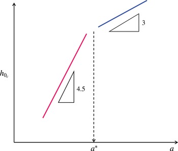
Figure 11. Sketch of how the critical film thickness
 $h_{0c}$
varies with the fibre radius
$h_{0c}$
varies with the fibre radius
 $a$
(in log–log scale). For large fibres with
$a$
(in log–log scale). For large fibres with
 $a>a^{\ast }$
, the no-slip result
$a>a^{\ast }$
, the no-slip result
 $h_{0c}\propto a^{3}$
dominates (see (6.2)). However, if the fibre size is reduced to
$h_{0c}\propto a^{3}$
dominates (see (6.2)). However, if the fibre size is reduced to
 $a<a^{\ast }$
, the strong-slip result
$a<a^{\ast }$
, the strong-slip result
 $h_{0c}\propto a^{9/2}$
will dominate instead (see (6.1)), where
$h_{0c}\propto a^{9/2}$
will dominate instead (see (6.1)), where
 $a^{\ast }=(\unicode[STIX]{x1D706}\unicode[STIX]{x1D705}^{-2})^{1/3}$
marks the critical fibre radius for the stick–slip transition with
$a^{\ast }=(\unicode[STIX]{x1D706}\unicode[STIX]{x1D705}^{-2})^{1/3}$
marks the critical fibre radius for the stick–slip transition with
 $\unicode[STIX]{x1D705}^{-1}=(\unicode[STIX]{x1D6FE}/\unicode[STIX]{x1D70C}g)^{1/2}$
being the capillary length.
$\unicode[STIX]{x1D705}^{-1}=(\unicode[STIX]{x1D6FE}/\unicode[STIX]{x1D70C}g)^{1/2}$
being the capillary length.
Another way to see how wall slip affects the coating is to look at the short-term film thinning kinetics. Neglecting the surface tension terms (i.e. omitting undulations of the interface), equation (2.9) is reduced to
 $$\begin{eqnarray}h_{t}+\left(h^{3}+\unicode[STIX]{x1D6EC}h^{2}\right)_{x}G=0.\end{eqnarray}$$
For small
 $\unicode[STIX]{x1D6EC}$
,
$\unicode[STIX]{x1D6EC}$
,
 $h_{t}+G(h^{3})_{x}=0$
leads the film to thin according to
$h_{t}+G(h^{3})_{x}=0$
leads the film to thin according to
 $h\propto t^{-1/2}$
, just like what Quéré observed. But when the film thins to the point where it becomes thinner than
$h\propto t^{-1/2}$
, just like what Quéré observed. But when the film thins to the point where it becomes thinner than
 $\unicode[STIX]{x1D706}$
, the thinning kinetics is governed by
$\unicode[STIX]{x1D706}$
, the thinning kinetics is governed by
 $h_{t}+\unicode[STIX]{x1D6EC}G(h^{2})_{x}=0$
. This accelerates the thinning to
$h_{t}+\unicode[STIX]{x1D6EC}G(h^{2})_{x}=0$
. This accelerates the thinning to
 $h\propto t^{-1}$
, which is close to the data trend for later times as seen in figure 12 reported by Quéré. Quéré attributed this thinning acceleration to axial grooves on the fibres. Alternatively, this acceleration can be interpreted by slip effects. The slip effects here could be caused by the hydrophobic fibres made by nylon, surface grooves, the silicone oil or their combination. Together with the fact that the measured
$h\propto t^{-1}$
, which is close to the data trend for later times as seen in figure 12 reported by Quéré. Quéré attributed this thinning acceleration to axial grooves on the fibres. Alternatively, this acceleration can be interpreted by slip effects. The slip effects here could be caused by the hydrophobic fibres made by nylon, surface grooves, the silicone oil or their combination. Together with the fact that the measured
 $G_{c}=0.71$
is slightly greater than
$G_{c}=0.71$
is slightly greater than
 $G_{c}=0.5960$
for no-slip fibres, all these deviations found in Quéré’s experiment can be well explained by wall slip effects.
$G_{c}=0.5960$
for no-slip fibres, all these deviations found in Quéré’s experiment can be well explained by wall slip effects.

Figure 12. Temporal evolution of the film thickness measured by Quéré (Reference Quéré1990), adapted from his figure 1. The film thinning kinetics can be accelerated from no-slip
 $h\propto t^{-1/2}$
to strong slip
$h\propto t^{-1/2}$
to strong slip
 $h\propto t^{-1}$
at late times.
$h\propto t^{-1}$
at late times.
7 Concluding remarks
We have demonstrated that wall slip can promote drop formation along a vertical fibre. Both the drop height and falling speed can be significantly increased with the amount of wall slip. In particular, when slip effects become strong, the critical Bond number
 $G_{c}$
for drop formation is found to increase with
$G_{c}$
for drop formation is found to increase with
 $\unicode[STIX]{x1D6EC}$
as
$\unicode[STIX]{x1D6EC}$
as
 $G_{c}\approx 0.7\unicode[STIX]{x1D6EC}^{1/3}$
. The
$G_{c}\approx 0.7\unicode[STIX]{x1D6EC}^{1/3}$
. The
 $\unicode[STIX]{x1D6EC}^{1/3}$
factor then leads the critical film thickness to vary with the fibre radius as
$\unicode[STIX]{x1D6EC}^{1/3}$
factor then leads the critical film thickness to vary with the fibre radius as
 $h_{0c}\propto a^{9/2}$
, more sensitive than the no-slip result
$h_{0c}\propto a^{9/2}$
, more sensitive than the no-slip result
 $h_{0c}\propto a^{3}$
. Such a sensitivity to the fibre radius due to wall slip explains why
$h_{0c}\propto a^{3}$
. Such a sensitivity to the fibre radius due to wall slip explains why
 $G_{c}$
found by Quéré (Reference Quéré1990) is slightly greater than that predicted by the no-slip model. The
$G_{c}$
found by Quéré (Reference Quéré1990) is slightly greater than that predicted by the no-slip model. The
 $\unicode[STIX]{x1D6EC}^{1/3}$
factor might come from changes of two length scales when wall slip effects become strong: (i)
$\unicode[STIX]{x1D6EC}^{1/3}$
factor might come from changes of two length scales when wall slip effects become strong: (i)
 $O(\unicode[STIX]{x1D6EC}^{1/3}c^{-1/3})$
for the transition film regions ahead and behind the main drop; and (ii)
$O(\unicode[STIX]{x1D6EC}^{1/3}c^{-1/3})$
for the transition film regions ahead and behind the main drop; and (ii)
 $O(\unicode[STIX]{x1D6EC}^{-2/3}c^{2/3})$
for the drop height. These are very distinct from those for the no-slip case in which the transition film regions are
$O(\unicode[STIX]{x1D6EC}^{-2/3}c^{2/3})$
for the drop height. These are very distinct from those for the no-slip case in which the transition film regions are
 $O(c^{-1/3})$
and the drop height is
$O(c^{-1/3})$
and the drop height is
 $O(c^{2/3})$
(Yu & Hinch Reference Yu and Hinch2013). We also find that the film thinning kinetics can be accelerated from no-slip
$O(c^{2/3})$
(Yu & Hinch Reference Yu and Hinch2013). We also find that the film thinning kinetics can be accelerated from no-slip
 $h\propto t^{-1/2}$
to strong slip
$h\propto t^{-1/2}$
to strong slip
 $h\propto t^{-1}$
at late times, in accordance with Quéré’s experiment. When the film is ultrathin, although strong slip effects can amplify capillary instability to make the film more susceptible to drop formation, this effect can be inhibited by equally intensified gravity draining through the KS mechanism.
$h\propto t^{-1}$
at late times, in accordance with Quéré’s experiment. When the film is ultrathin, although strong slip effects can amplify capillary instability to make the film more susceptible to drop formation, this effect can be inhibited by equally intensified gravity draining through the KS mechanism.
It is worth remarking that the present analysis is more suitable for the situation where apparent slip is generated by a polymeric liquid as in Quéré’s experiment. For a flow over a rough or textured surface, however, the effective slip length can only be defined when the film is much thicker than the size of the roughness. Hence, if the film is much thinner than the size of roughness, our analysis will no longer be applicable.
Acknowledgement
This work was supported by the Ministry of Science and Technology of Taiwan under grant no. 105-2221-E-006-227-MY3 of H.-H.W.
Appendix A
The numerical method used to solve (2.10) is similar to that described in Yu & Hinch (Reference Yu and Hinch2013). As the uniform film regions are approached, asymptotic solutions can be obtained by linearizing (2.10) about
 $h=1$
. Letting
$h=1$
. Letting
 $h=1+\unicode[STIX]{x1D6FF}\unicode[STIX]{x1D702}$
where
$h=1+\unicode[STIX]{x1D6FF}\unicode[STIX]{x1D702}$
where
 $\unicode[STIX]{x1D6FF}\ll 1$
, to leading order
$\unicode[STIX]{x1D6FF}\ll 1$
, to leading order
 $\unicode[STIX]{x1D702}$
satisfies
$\unicode[STIX]{x1D702}$
satisfies
 $$\begin{eqnarray}\unicode[STIX]{x1D702}_{xxx}+\unicode[STIX]{x1D702}_{x}+\frac{1}{1+\unicode[STIX]{x1D6EC}}\left((3+2\unicode[STIX]{x1D6EC})G-c\right)\unicode[STIX]{x1D702}=0.\end{eqnarray}$$
This equation has solutions of the form
 $\text{e}^{mx}$
where
$\text{e}^{mx}$
where
 $m$
satisfies the cubic equation
$m$
satisfies the cubic equation
 $$\begin{eqnarray}m^{3}+m+\frac{1}{1+\unicode[STIX]{x1D6EC}}\left((3+2\unicode[STIX]{x1D6EC})G-c\right)=0.\end{eqnarray}$$
If the constant term of the cubic is positive, that is when
 $c<(3+2\unicode[STIX]{x1D6EC}G)$
, this equation has one positive real root,
$c<(3+2\unicode[STIX]{x1D6EC}G)$
, this equation has one positive real root,
 $m_{+}$
, which yields an exponentially decaying solution as
$m_{+}$
, which yields an exponentially decaying solution as
 $x\rightarrow -\infty$
of the form
$x\rightarrow -\infty$
of the form
 $A\text{e}^{m_{+}x}$
, and two complex conjugate roots with negative real parts,
$A\text{e}^{m_{+}x}$
, and two complex conjugate roots with negative real parts,
 $\unicode[STIX]{x1D6FC}\pm \text{i}\unicode[STIX]{x1D6FD}$
, that give rise to two oscillatory solutions that decay as
$\unicode[STIX]{x1D6FC}\pm \text{i}\unicode[STIX]{x1D6FD}$
, that give rise to two oscillatory solutions that decay as
 $x\rightarrow \infty$
of the form
$x\rightarrow \infty$
of the form
 $B\text{e}^{\unicode[STIX]{x1D6FC}x}\cos (\unicode[STIX]{x1D6FD}x+k)$
where
$B\text{e}^{\unicode[STIX]{x1D6FC}x}\cos (\unicode[STIX]{x1D6FD}x+k)$
where
 $A$
,
$A$
,
 $B$
and
$B$
and
 $k$
are constants.
$k$
are constants.
Equation (2.10) is rewritten as a system of three first-order differential equations, and solved as an initial value problem using a Runge–Kutta method (ODE45 from MATLAB). Let
 $h_{1}$
be the solution of (2.10) with the initial condition specified at
$h_{1}$
be the solution of (2.10) with the initial condition specified at
 $x=-d_{1}$
coming from the monotonically decaying solution as
$x=-d_{1}$
coming from the monotonically decaying solution as
 $x\rightarrow -\infty$
, and let
$x\rightarrow -\infty$
, and let
 $h_{2}$
be the solution of (2.10) with the initial condition specified at
$h_{2}$
be the solution of (2.10) with the initial condition specified at
 $x=d_{2}$
coming from the oscillatory decaying solution as
$x=d_{2}$
coming from the oscillatory decaying solution as
 $x\rightarrow \infty$
. We stop computing
$x\rightarrow \infty$
. We stop computing
 $h_{1}$
and
$h_{1}$
and
 $h_{2}$
at
$h_{2}$
at
 $x=d$
, a point in the middle of the drop where
$x=d$
, a point in the middle of the drop where
 $h$
is not too close to
$h$
is not too close to
 $1$
, and require
$1$
, and require
 $h$
and
$h$
and
 $h_{x}$
to be continuous and
$h_{x}$
to be continuous and
 $h_{xx}=0$
there, i.e.
$h_{xx}=0$
there, i.e.
 $h_{1}(d)=h_{2}(d)$
,
$h_{1}(d)=h_{2}(d)$
,
 $h_{1x}(d)=h_{2x}(d)$
,
$h_{1x}(d)=h_{2x}(d)$
,
 $h_{1xx}(d)=0$
and
$h_{1xx}(d)=0$
and
 $h_{2xx}(d)=0$
. An iterative scheme based on a Newton’s method is applied that adjusts the speed
$h_{2xx}(d)=0$
. An iterative scheme based on a Newton’s method is applied that adjusts the speed
 $c$
and the amplitude of the oscillatory decaying solution until the matching conditions are satisfied.
$c$
and the amplitude of the oscillatory decaying solution until the matching conditions are satisfied.
Appendix B
Let
 $x=x_{0}+c^{-1/3}\unicode[STIX]{x1D709}$
. Then (2.10) becomes
$x=x_{0}+c^{-1/3}\unicode[STIX]{x1D709}$
. Then (2.10) becomes
 $$\begin{eqnarray}h_{\unicode[STIX]{x1D709}\unicode[STIX]{x1D709}\unicode[STIX]{x1D709}}=\frac{h-1}{h^{3}+\unicode[STIX]{x1D6EC}h^{2}}-c^{-2/3}h_{\unicode[STIX]{x1D709}}+c^{-1}G\frac{1-h^{3}+\unicode[STIX]{x1D6EC}(1-h^{2})}{h^{3}+\unicode[STIX]{x1D6EC}h^{2}}.\end{eqnarray}$$
For
 $c\gg 1$
, the leading order problem is
$c\gg 1$
, the leading order problem is
 $$\begin{eqnarray}h_{\unicode[STIX]{x1D709}\unicode[STIX]{x1D709}\unicode[STIX]{x1D709}}=\frac{h-1}{h^{3}+\unicode[STIX]{x1D6EC}h^{2}}.\end{eqnarray}$$
The above equation is solved subject to matching conditions with the uniform film regions, where
 $h\rightarrow 1$
. Letting
$h\rightarrow 1$
. Letting
 $h=1+\unicode[STIX]{x1D6FF}\unicode[STIX]{x1D702}$
where
$h=1+\unicode[STIX]{x1D6FF}\unicode[STIX]{x1D702}$
where
 $\unicode[STIX]{x1D6FF}\ll 1$
,
$\unicode[STIX]{x1D6FF}\ll 1$
,
 $\unicode[STIX]{x1D702}_{\unicode[STIX]{x1D709}\unicode[STIX]{x1D709}\unicode[STIX]{x1D709}}=\unicode[STIX]{x1D702}/(1+\unicode[STIX]{x1D6EC})$
, whose solutions are
$\unicode[STIX]{x1D702}_{\unicode[STIX]{x1D709}\unicode[STIX]{x1D709}\unicode[STIX]{x1D709}}=\unicode[STIX]{x1D702}/(1+\unicode[STIX]{x1D6EC})$
, whose solutions are
 $$\begin{eqnarray}\text{e}^{\unicode[STIX]{x1D709}/(1+\unicode[STIX]{x1D6EC})^{1/3}},\quad \text{e}^{-\unicode[STIX]{x1D709}/2(1+\unicode[STIX]{x1D6EC})^{1/3}}\cos \left(\frac{\sqrt{3}}{2}\frac{\unicode[STIX]{x1D709}}{(1+\unicode[STIX]{x1D6EC})^{1/3}}\right),\quad \text{e}^{-\unicode[STIX]{x1D709}/2(1+\unicode[STIX]{x1D6EC})^{1/3}}\sin \left(\frac{\sqrt{3}}{2}\frac{\unicode[STIX]{x1D709}}{(1+\unicode[STIX]{x1D6EC})^{1/3}}\right).\end{eqnarray}$$
The appropriate asymptotic solution to match with the rear uniform film is the first one given in (B 3), which is a purely decaying mode there, while in the front uniform film, we retain the other two solutions since they decay as
 $\unicode[STIX]{x1D709}\rightarrow \infty$
. From (B 2), in the large drop region, where
$\unicode[STIX]{x1D709}\rightarrow \infty$
. From (B 2), in the large drop region, where
 $h\gg 1$
, the curvature is constant to leading order. Also, the profiles approaching the large drop from either the front or rear transition regions can be described by parabolas of the form
$h\gg 1$
, the curvature is constant to leading order. Also, the profiles approaching the large drop from either the front or rear transition regions can be described by parabolas of the form
 $$\begin{eqnarray}h\sim {\textstyle \frac{1}{2}}P_{\pm }\unicode[STIX]{x1D709}^{2}+R_{\pm }={\textstyle \frac{1}{2}}c^{2/3}P_{\pm }\left(x-x_{0}\right)^{2}+R_{\pm },\end{eqnarray}$$
where, by a suitable choice of the origin, equation (B 4) has no linear term in
 $\unicode[STIX]{x1D709}$
. For a given
$\unicode[STIX]{x1D709}$
. For a given
 $\unicode[STIX]{x1D6EC}$
, equation (B 2) is solved numerically using the purely decaying mode given in (B 3) as an initial condition for the left transition region. This numerical solution is matched with the large constant curvature drop as
$\unicode[STIX]{x1D6EC}$
, equation (B 2) is solved numerically using the purely decaying mode given in (B 3) as an initial condition for the left transition region. This numerical solution is matched with the large constant curvature drop as
 $\unicode[STIX]{x1D709}\rightarrow \infty$
, yielding values for
$\unicode[STIX]{x1D709}\rightarrow \infty$
, yielding values for
 $P_{+}$
and
$P_{+}$
and
 $R_{+}$
. In the front (or right) transition region, the initial condition for
$R_{+}$
. In the front (or right) transition region, the initial condition for
 $h$
is expressed as a combination of the two oscillatory solutions in (B 3),
$h$
is expressed as a combination of the two oscillatory solutions in (B 3),
 $$\begin{eqnarray}h\approx 1+A_{f}\text{e}^{-\unicode[STIX]{x1D709}/2(1+\unicode[STIX]{x1D6EC})^{1/3}}\cos \left(\frac{\sqrt{3}}{2}\frac{\unicode[STIX]{x1D709}}{(1+\unicode[STIX]{x1D6EC})^{1/3}}+\unicode[STIX]{x1D719}\right),\end{eqnarray}$$
where
 $A_{f}$
and
$A_{f}$
and
 $\unicode[STIX]{x1D719}$
are the amplitude (chosen to be small) and a phase difference. The latter provides an extra degree of freedom in comparison with the rear transition region. Numerically, it is adjusted using a Newton’s method until
$\unicode[STIX]{x1D719}$
are the amplitude (chosen to be small) and a phase difference. The latter provides an extra degree of freedom in comparison with the rear transition region. Numerically, it is adjusted using a Newton’s method until
 $P_{-}=P_{+}$
, so that the pressure is continuous.
$P_{-}=P_{+}$
, so that the pressure is continuous.
As explained by Yu & Hinch (Reference Yu and Hinch2013), from the perspective of the large drop, the constant terms in (B 4) denote the thicknesses of the uniform films. The critical
 $G$
can be obtained from the following relationship
$G$
can be obtained from the following relationship
 $$\begin{eqnarray}G=\frac{R_{+}-R_{-}}{2\unicode[STIX]{x03C0}}.\end{eqnarray}$$


